Chapter 5
Audio Processing Systems
U. Zölzer and D. Ahlers
The techniques, systems, and devices for digital audio processing have substantially changed over the past decades and have now reached a status where software‐based systems have pushed hardware‐based systems almost off of the processing chain. Most of the processing can now be done on general purpose personal computers or tablet computers. All kinds of interfacing of microphones and loudspeakers to the computer world still need dedicated hardware solutions. Lately, microphones and loudspeakers have been improved by digital signal processing and such low‐power devices need specialized hardware such as digital signal processors (DSPs) or field programmable gate arrays (FPGAs). Large‐scale mixing consoles are still benefiting from hardware integration using FPGAs for interfacing and internal multiple signal processing cores. The obvious trend is toward higher integration density and smaller hardware devices integrated into audio networks.
New DSPs with extended interfaces are still used in different application areas where a computer is bulky and excessive. Newer DSPs offer a variety of interfaces to analog‐to‐digital convertors (ADCs)/digital‐to‐analog convertors (DACs), local area networks (LANs), and wireless local area networks (WLANs), which make them very attractive for innovative audio designs with low‐power consumption and low latency. An overview of processing devices is shown in Table 5.1. New software‐based audio systems have benefited from the progress of computer technology with different operating systems. Audio processing on central processing units (CPUs) and graphics processing units (GPUs) have impressively accelerated audio computing and recording. The range of devices from mobile phones over tablet computers to general purpose computers are all suitable for dedicated audio processing tasks but, of course, there is still a requirement for the sophisticated skills of software programmers.
Table 5.1 DSPs (AD/TI/NXP/STM/Cadence/Xilinx) and applications
| System on a chip | Floating‐point | Fixed‐point | Field Program. |
|---|---|---|---|
| LAN/WLAN | DSPs | DSPs | Gate Arrays |
| Raspberry Pi | PC/CPU/GPU | Sigmastudio | Xilinx |
| streaming | DAWs | headphones | microphones |
| networking | synthesizers | loudspeakers | mixing consoles |
| wireless speaker | recording | synthesizers | |
| systems | mixing | effects | |
| mastering | |||
| block latency | block latency | 1–2 samples | 0 samples |
5.1 Digital Signal Processors
5.1.1 Fixed‐point DSPs
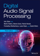
The discrete‐time and discrete‐amplitude output of an AD converter is usually represented in 2's‐complement format. The processing of these number sequences is carried out with fixed‐point or floating‐point arithmetic. The output of a processed signal is again in 2's‐complement format and is fed to a DA converter. The signed fractional representation (2's complement) is the common way for algorithms in fixed‐point number representation. To address the generation and modulo operations, unsigned integers are used. Figure 5.1 shows a schematic diagram of a typical fixed‐point DSP. The main building blocks are program controller, arithmetic logic unit (ALU) with a multiplier–accumulator (MAC), program and data memory, and interfaces to external memory and peripherals. All blocks are connected with each other by an internal bus system. The internal bus system has separate instruction and data buses. The data bus itself can consist of more than one parallel bus enabling it, for instance, to transmit both operands of a multiplication instruction to the MAC in parallel. The internal memory consists of instruction and data random access memory (RAM) and additional read‐only memory (ROM). This internal memory permits a fast execution of internal instructions and data transfer. To increase the memory space, address/control and data buses are connected to external memories like erasable programmable (EP)ROM, ROM, and RAM. The connection of the external bus system to the internal bus architecture has a great influence on the efficient execution of external instructions as well as on processing external data. To connect serially operating AD/DA converters, special serial interfaces with high transmission rates are offered by several DSPs. Moreover, some processors support direct connection to an RS232 interface. The control from a microprocessor can be achieved via a host interface with a word length of 8 bits.
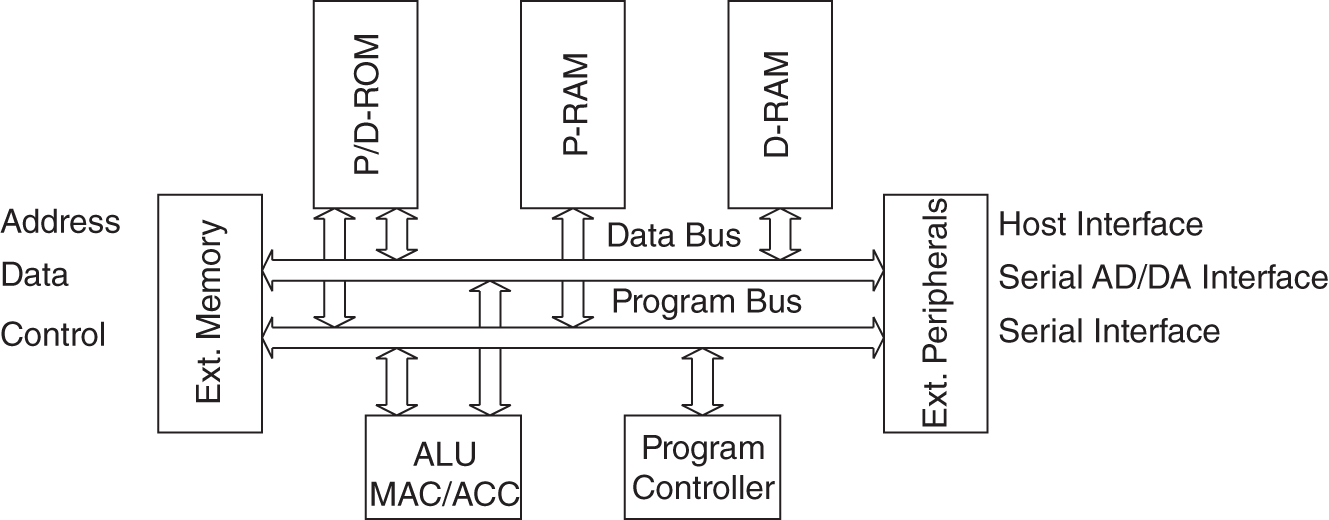
Figure 5.1 Schematic diagram of a fixed‐point DSP.
An overview of fixed‐point DSPs with respect to word length and cycle time can be explored from the websites of the corresponding manufacturers. Basically, the precision of the arithmetic can be doubled if quantization affects the stability and numeric precision of the applied algorithm. The cycle time in connection with processing time (in processor cycles) of a combined multiplication and accumulation command gives insight into the computing power of a particular processor type. The cycle time directly results from the maximum clock frequency. The instruction processing time depends mainly on the internal instruction and data structure, as well as on the external memory connections of the processor. The fast access to external instruction and data memories is of special significance in complex algorithms and in processing huge data loads. Further attention has to be paid to the linking of serial data connections with AD/DA converters and the control by a host computer over a special host interface. Complex interface circuits could therefore be avoided. For stand‐alone solutions, program loading from a simple external EPROM can also be done.
For signal processing algorithms, the following software commands are necessary:
- MAC (multiply and accumulate)
 combined multiplication and addition command;
 - simultaneous transfer of both operands for multiplication to the MAC (parallel move);
- bit‐reversed addressing (for fast Fourier transfer (FFT));
- modulo addressing (for windowing and filtering).
Different signal processors have different processing times for FFT implementations. The latest signal processors with improved architecture have shorter processing times. The instruction cycles for the combined multiplication and accumulation command (application: windowing, filtering) are approximately equal for different processors, but processing cycles for external operands have to be considered.
5.1.2 Floating‐point DSPs
Figure 5.2 shows the block diagram of a typical floating‐point DSP. The main characteristics of the different architectures are the dual‐port principle (Texas Instruments) and the external Harvard architecture (Analog Devices). Floating‐point DSPs internally have multiple bus systems to accelerate data transfer to the processing unit. An on‐chip direct memory access (DMA) controller and cache‐memory support higher data transfer rates.
5.2 Digital Audio Interfaces
For transferring digital audio signals, two transmission standards have been established by the AES (Audio Engineering Society) and the EBU (European Broadcasting Union). These standards are for two‐channel transmission [AES3] and for multi‐channel transmission of up to 64 audio channels [AES10], known as a multichannel audio digital interface (MADI).

Figure 5.2 Block diagram of a floating‐point digital signal processor.
5.2.1 Two‐channel AES/EBU Interface
For the two‐channel AES/EBU (also known as AES3) interface, professional and consumer modes are defined. The outer frame is identical for both modes and is shown in Fig. 5.3. For a sampling period, a frame is defined so that it consists of two subframes, for channel 1 with preamble X and for channel 2 with preamble Y. A total of 192 frames form a block. The block start is characterized by a special preamble Z. The bit allocation of a subframe consists of 32 bits, as shown in Fig. 5.4. The preamble consists of 4 bits (bits 0–3) and the audio data of up to 24 bits (bits 4–27). The last four bits of the subframe characterize Validity (validity of data word or error), User Status (usable bit), Channel Status (from ![]() bytes coded status information for the channel), and Parity (even parity). The transmission of the serial data bits is carried out with a bi‐phase mark code. This is done with the help of an XOR relationship between clock (of double bit rate) and the serial data bits (Fig. 5.5). At the receiver, clock retrieval is achieved by detecting the preamble (X=11100010, Y=11100100, Z=11101000) as it violates the coding rule (see Fig. 5.6). The meaning of the 24 bytes for channel status information is summarized in Table 5.2. An exact bit allocation of the first three important bytes of this channel status information is presented in Fig. 5.7. In the individual fields of byte 0, pre‐emphasis and sampling rate are specified in addition to professional/consumer modes and the characterization of data/audio (see Tables 5.3 and 5.4). Byte 1 determines the channel mode (Table 5.5). The consumer format (often labeled as SPDIF, Sony/Philips Digital Interface Format) differs from the professional format in the definition of the channel status information and the technical specifications for inputs and outputs. The bit allocation for the first four bits of the channel information is shown in Fig. 5.8. For consumer applications, a coaxial cable with RCA connectors or a fiber optic cable with TOSLINK connectors are used. For professional use, shielded two‐wired leads with XLR connectors and symmetrical inputs and outputs (professional format) are used. Table 5.6 shows the electrical specifications for professional AES/EBU interfaces.
bytes coded status information for the channel), and Parity (even parity). The transmission of the serial data bits is carried out with a bi‐phase mark code. This is done with the help of an XOR relationship between clock (of double bit rate) and the serial data bits (Fig. 5.5). At the receiver, clock retrieval is achieved by detecting the preamble (X=11100010, Y=11100100, Z=11101000) as it violates the coding rule (see Fig. 5.6). The meaning of the 24 bytes for channel status information is summarized in Table 5.2. An exact bit allocation of the first three important bytes of this channel status information is presented in Fig. 5.7. In the individual fields of byte 0, pre‐emphasis and sampling rate are specified in addition to professional/consumer modes and the characterization of data/audio (see Tables 5.3 and 5.4). Byte 1 determines the channel mode (Table 5.5). The consumer format (often labeled as SPDIF, Sony/Philips Digital Interface Format) differs from the professional format in the definition of the channel status information and the technical specifications for inputs and outputs. The bit allocation for the first four bits of the channel information is shown in Fig. 5.8. For consumer applications, a coaxial cable with RCA connectors or a fiber optic cable with TOSLINK connectors are used. For professional use, shielded two‐wired leads with XLR connectors and symmetrical inputs and outputs (professional format) are used. Table 5.6 shows the electrical specifications for professional AES/EBU interfaces.
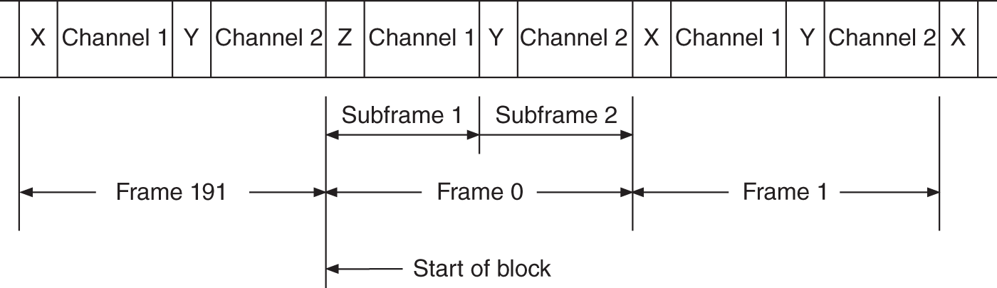
Figure 5.3 Two‐channel format.
Figure 5.4 Two‐channel format (subframe).
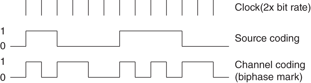
Figure 5.5 Channel coding.

Figure 5.6 Preamble X.
5.2.2 MADI Interface
To connect an audio processing system at different locations, a MADI interface is used [AES10]. A system link by MADI is presented in Fig. 5.9. Analog/digital I/O systems consisting of AD/DA converters, AES/EBU interfaces (AES), and sampling rate converters (SRC) are connected to digital distribution systems with bi‐directional MADI links. The actual audio signal processing is performed in special DSP systems which are connected to the digital distribution systems by MADI links. The MADI format is standardized as AES10 and is derived from the two‐channel AES/EBU format and allows the transmission of 64 digital mono channels (see Fig. 5.10) within a sampling period. The MADI frame consists of 64 AES/EBU subframes. Each channel has a preamble containing the information shown in Fig. 5.10. The bit 0 is responsible for identifying the first MADI channel (MADI Channel 0). Table 5.7 shows the sampling rates and the corresponding data transfer rates. The maximum data rate of 98.304 Mbit/s is required at a sampling rate of 48 kHz. The transmission is done via 75‐Ohm coaxial cables with BNC connectors (50 m, signal amplitude 0.3–0.6 V) or via fiber optic lines with SC connectors (up to 2 km).
Table 5.2 Channel status bytes
| Byte | Description |
|---|---|
| 0 | emphasis, sampling rate |
| 1 | channel use |
| 2 | sample length |
| 3 | vector for byte 1 |
| 4 | reference bits |
| 5 | reserved |
| 6–9 | 4 bytes of ASCII origin |
| 10–13 | 4 bytes of ASCII destination |
| 14–17 | 4 bytes of local address |
| 18–21 | time code |
| 22 | flags |
| 23 | CRC |
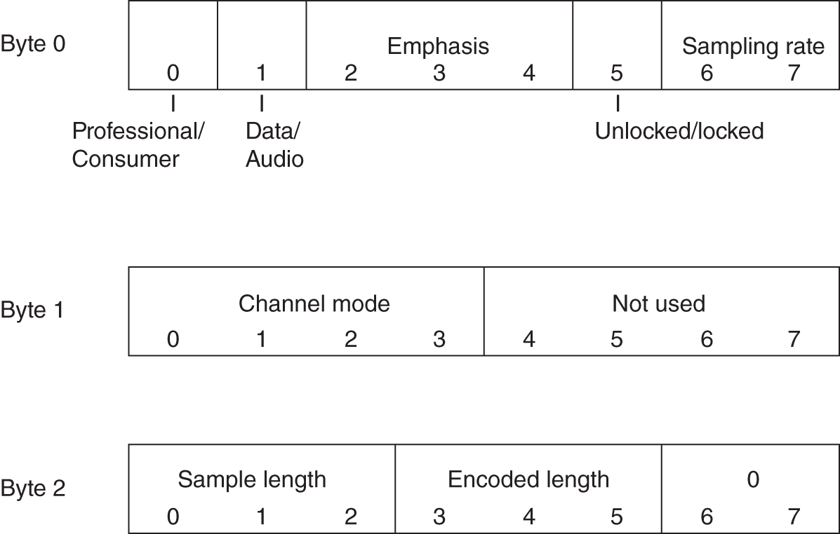
Figure 5.7 Bytes 0–2 of channel status information.
Table 5.3 Emphasis field
| 0 | none indicated, override enabled |
| 4 | none indicated, override disabled |
| 6 | 50/15 |
| 7 | CCITT J.17 emphasis |
Table 5.4 Sampling rate field
| 0 | none indicated (48 kHz default) |
| 1 | 48 kHz |
| 2 | 44.1 kHz |
| 3 | 32 kHz |
Table 5.5 Channel mode
| 0 | none indicated (2 channel default) |
| 1 | two channel |
| 2 | monaural |
| 3 | primary/secondary (A=primary, B=secondary) |
| 4 | stereo (A=left, B=right) |
| 7 | vector to byte 3 |
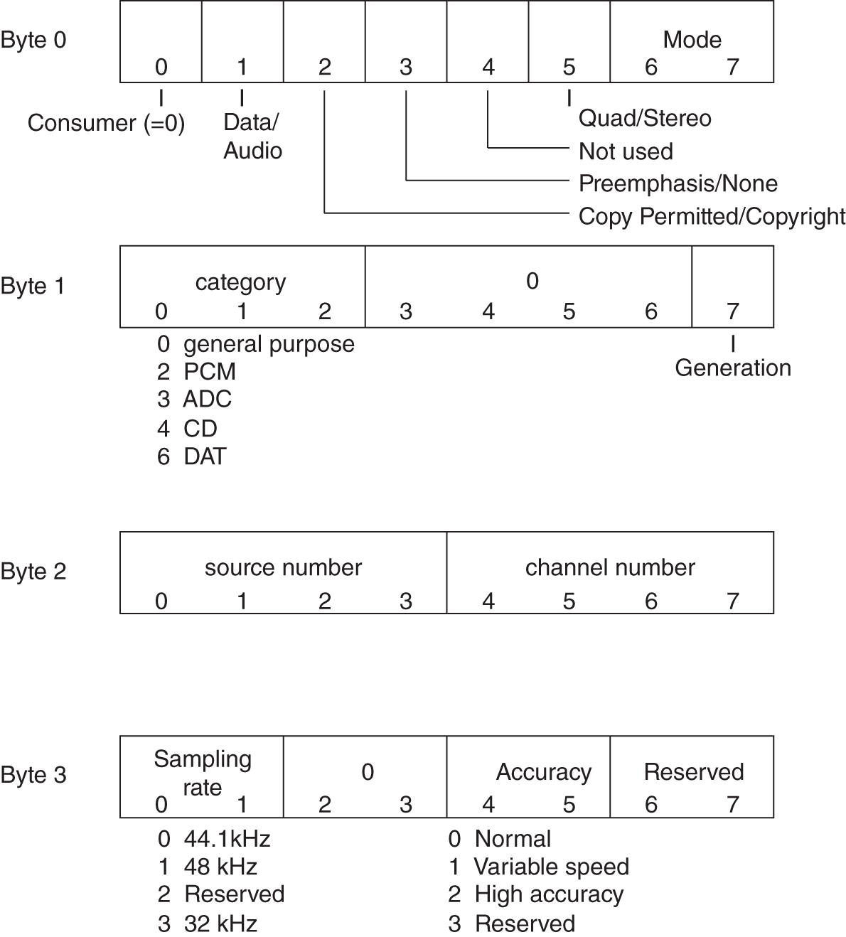
Figure 5.8 Bytes 0–3 (consumer format).
Table 5.6 Electrical specifications of professional interfaces
| Output impedance | Signal amplitude | Jitter |
|---|---|---|
| 110 | 2–7 V | max. 20 ns |
| Input impedance | Signal amplitude | Connect. |
| 110 | min. 200 mV | XLR |
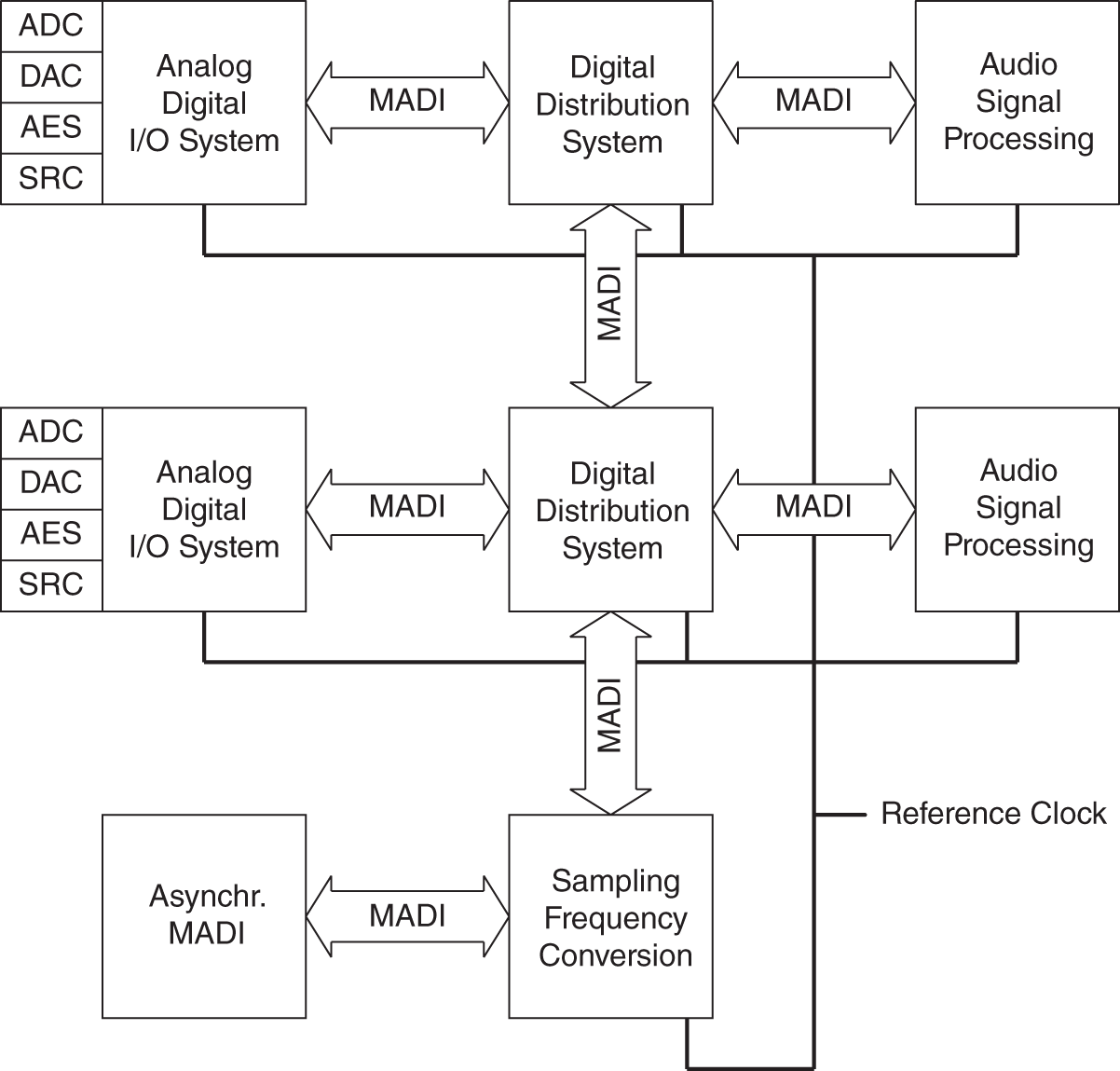
Figure 5.9 A system link by MADI.

Figure 5.10 MADI frame format.
Table 5.7 MADI specifications
| Sampling rate | 32–48 kHz |
| Transmission rate | 125 Mbit/s |
| Data transfer rate | 100 Mbit/s |
| Max. data transfer rate | 98.304 Mbit/s (64 channels at 48 kHz) |
5.2.3 Audio in HDMI
High‐definition multimedia interface (HDMI) is a proprietary audio/video interface standard. The digital audio data are sent, combined together with video and auxiliary data, within the tree TMDS (transition minimized differential signaling) data channels, as depicted in Fig. 5.11. Figure 5.12 shows the physical pinout of the channels, where one can see that each TMDS channel is separately shielded and transmitted as a differential signal over a twisted pair. The audio data can consist of any compressed, uncompressed, pulse code modulation (PCM), single or multichannel format of up to 8 channels (since HDMI 2.0, 32 channels) and is being transmitted during the video blanking intervals encapsulated inside the so called data island period 1. To make sure the transmitter only sends audio or video data, the receiver is capable of receiving, there is an information exchange in the display data channel (DDC) that is ![]() C‐based during the connection establishment. The standard for that is called extended display identification data (EDID) and is published by the Video Electronics Standards Association (VESA). It contains the manufacturer ID and model name as well as information of the capable video formats like resolution, aspect ratio, bit depth, and refresh rate. The audio descriptor of the EDID contains information like audio format, number of channels, sampling rate, and bit depth.
C‐based during the connection establishment. The standard for that is called extended display identification data (EDID) and is published by the Video Electronics Standards Association (VESA). It contains the manufacturer ID and model name as well as information of the capable video formats like resolution, aspect ratio, bit depth, and refresh rate. The audio descriptor of the EDID contains information like audio format, number of channels, sampling rate, and bit depth.
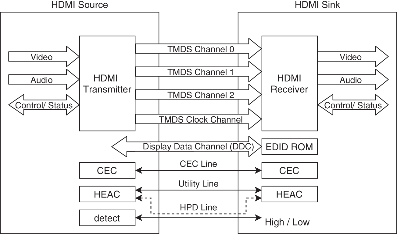
Figure 5.11 HDMI block diagram.
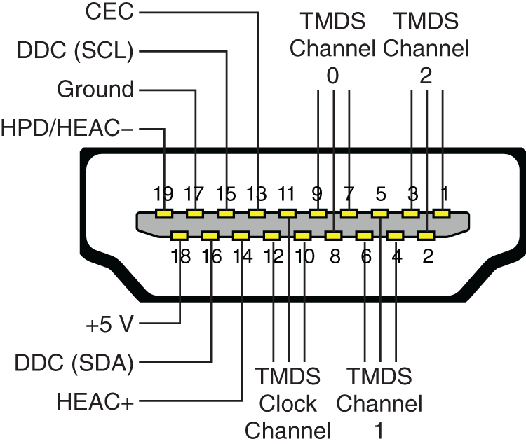
Figure 5.12 HDMI pinout since HDMI 1.4.
In addition to the audio transmission from the transmitter to the receiver, HDMI specifies an audio transmission from the receiver back to the transmitter, called audio return channel (ARC), a feature of HDMI 1.4a and an updated version called eARC (enhanced ARC) since HDMI 2.1. This is useful if an AV receiver is connected to a TV as display output but the TV is the source of the signal, for example when receiving a television program. Then the audio of the television program can be sent back to the AV receiver within the same HDMI cable. ARC is carried together with an Ethernet connection on the HDMI Ethernet and audio return channel (HEAC), a separate connection in an HDMI cable. HEAC shares the pin with the HPD (hot plug detection), as depicted in Fig. 5.12. The remaining unexplained connection in Fig. 5.11 is the consumer electronics control (CEC). A bidirectional connection that makes it possible to control all connected HDMI devices by using only on remote control.
Currently, the maximum data rate that can be transmitted over HDMI is ![]() Gbit/s defined by the HDMI 2.1 standard2.
Gbit/s defined by the HDMI 2.1 standard2.
5.2.4 Audio Computer Interfaces
There are several computer interfaces for audio, the most common being:
- Universal Serial Bus (USB) (device class definition for audio data formats3);
- Thunderbolt;
- Bluetooth audio.
In particular, USB and Thunderbolt allow a high data rate (see Table 5.8) and therefore a high number of audio channels for both input and output signals. For comparison, a common sampling rate of 48 kHz @ 24 bits needs 1.152 Mbit/s. Even professional audio recordings with a sampling rate of 192 kHz @ 24 bits only create 4.608 Mbit/s of pure data. The audio data will be transmitted uncompressed as PCM values, which are divided into blocks.
Table 5.8 Computer interfaces
| Type | Bitrate |
|---|---|
| USB 2.0 | 480 Mbit/s |
| USB 3.0 | 5 Gbit/s |
| USB 3.1 | 10 Gbit/s |
| Thunderbolt 1.0 | 10 Gbit/s |
| Thunderbolt 2.0 | 20 Gbit/s |
| Thunderbolt 3.0 | 40 Gbit/s |
While Bluetooth offers a wireless communication widely used in the consumer market, USB and Thunderbolt are still in the lead for professional equipment. Both offer short‐range connection between external audio devices and the computer using specific interface cables. For longer ranges, network interfaces will become the main solution.
On the software side, a device driver is required that creates a software interface and makes the hardware accessible to the operation system (OS) and other programs. For audio devices, normally this driver talks to the OS audio engine. The audio engine then provides standard APIs for the applications. Over the past few years, multiple APIs have been created. A list of the most common ones is provided in Table 5.9 and there are a few more.
Table 5.9 Computer interfaces
| OS | Audio Engine |
|---|---|
| Linux | ALSA (Advanced Linux Sound Architecture) |
| OSS (Open Sound System) (outdated) | |
| Windows | ASIO (Audio Stream Input/Output) |
| WASAPI (Windows Audio Session API) to connect to | |
| WDM (Windows Driver Model) Audio drivers | |
| macOS and iOS | CoreAudio |
5.2.5 Audio Network Interfaces
Network interfaces for audio can be divided into two main use cases. For the first use case, network‐based audio protocols are described that are mainly used in LAN for audio transmission with specialized hardware interfaces. They are commonly used for live events or in recordings scenarios and they are increasingly replacing the analog audio transmission. Because low latency is very important in such scenarios and the data rate on LAN is not so small, audio is sent mostly uncompressed in packets as PCM values.
For the second use case, the more internet‐based audio protocols are described that are often only software based and normally used for telecommunication. It is a more general term for Voice‐over‐Internet Protocol (VoIP) and often combined with video in conferencing software. However, almost every live audio transmission like music streaming or online radio is done in a similar way. Because internet bandwidth is very costly, normally the audio gets compressed by encoding algorithms.
Network‐based audio
There is a very large number of network‐based audio protocols that are incompatible with each other. Some are open standards and some are proprietary, but they all share the same physical connection: Ethernet cables. These cables are mostly made from copper but fiber connections are also possible. The fundamental difference between the protocols is the used network layer on which they operate. This also defines the topology of the network, the interoperability to existing Ethernet networks, and can influence the reliability and latency. The protocols are grouped into layer‐1, layer‐2, and layer‐3 protocols. This categorization is based on the ISO OSI model.
Layer‐1 network protocol. This protocol only uses a physical connection of Ethernet cables but defines their own cable pin assignment and does not use the Ethernet frame structure. Therefore only point‐to‐point connections between special hardware that supports the protocol are used. This means every connection requires an additional wire. Because there is a dedicated network, it is possible to create a reliable connection with guaranteed latency. As an example, AES50 [AES50] is described in more detail here and a typical network for a live show recording is shown in Fig. 5.13. It is mostly used by the Music Tribe Group (Midas, Klark Teknik, Behringer).
- AES50 [AES50]
- Uses CAT5 copper cables up to 100 m (100 Mbit/s),
- 48 input /48 output channels @ 48 kHz/24 bit or
- 24 input /24 output channels channels @ 96 kHz/24 bits,
- 5 Mbit/s auxiliary data connection, for example, used for remote gain control of ADCs,
- latency
 s,
s, - uses AES/EBU streams (enhancement of AES10 / MADI),
- separate signal pairs for audio and sync connection.
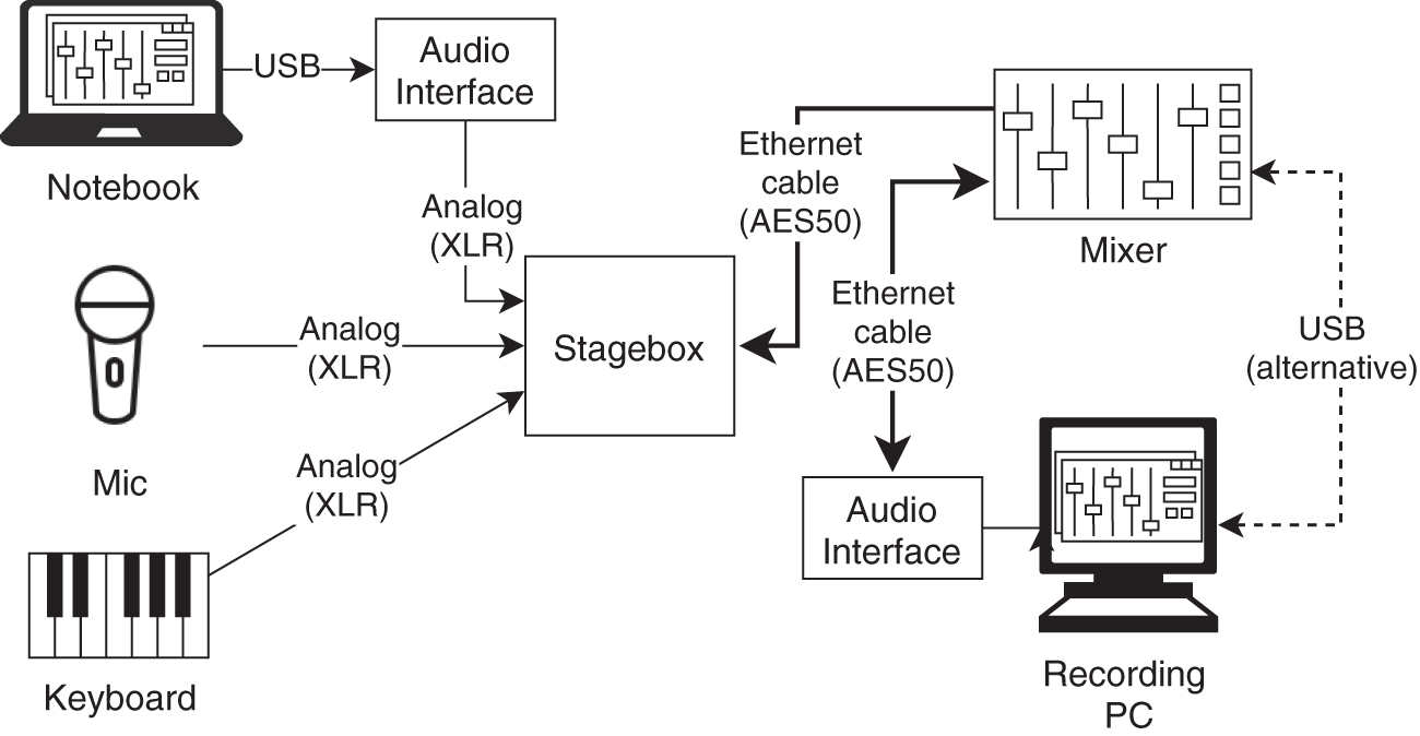
Figure 5.13 Example layer‐1 network (AES50 replaces the traditional multicore wires in this live scenario).
Layer‐2 network protocol. Audio data get encapsulated in Ethernet packages and can then be transmitted on an Ethernet network. However, because these packages are below the Internet Protocol (IP)‐level, special Ethernet hubs and switches are required that can handle the audio protocol and IP packets at the same time. As an example, AVB, the most prominent protocol that is layer‐2 based, is described here and a typical network for a live show recording is shown in Fig. 5.14.
- AVB (Audio Video Bridging)
- Key aspects: timing and synchronization, stream reservation protocol. Reliability and latency can be guaranteed.
- Requires special hardware to create a network (AVB compatible switches).
- Can coexist with an IP connection on the same link, if hardware supports it.
- Supports audio up to 196 kHz/32 bit.
- Multiple channels are encapsulated in AVB streams. One stream can contain up to 64 channels. With multiple streams between two devices, the number of channels is only limited by hardware limitations and link bandwidth.
- Typical interface: 128 input / 128 output channels @ 48 kHz/24 bit ( 14% utilization of 1 Gigabit Ethernet).
- 100 Mbit/s, 1 Gbit/s, or fiber connection possible.
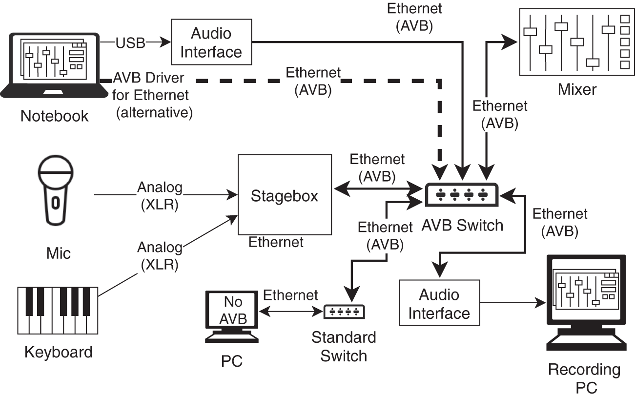
Figure 5.14 Example layer‐2 network (the PC cannot receive the AVB stream because it is connected via a standard router with no AVB support).
- Synchronization done via precision time protocol (PTP) with nanosecond precision.
- Network contains one Master clock that must be configured (primary clock) and the other devices as slaves (secondary clock).
- Network contains talker, listener, and AVB capable switches.
- Multiple stream reservation protocol (MSRP) used to reserve bandwidth throughout the entire network path.
- Bandwidth gets reserved before transmission and blocked, and is therefore guaranteed.
- Latency is, by default, bounded to 2 ms, which is comparable to 7 hops in a network. The playback will be delayed if the packet arrives earlier at the receiver. The advantage is that the delay is constant.
- AVB is defined in IEEE 802.1 (open standard, no license fee).
- Remote gain control can be done via IP link but is not defined in the standard and therefore may likely not be compatible among vendors.
Layer‐3 network protocol. Unlike the previous protocol standards, layer‐3 protocols can be easily integrated in existing local area networks with standard and therefore cheap hardware. One thing to keep in mind is that this protocol relays on the IP that only provides best‐effort delivery and is, by design, unreliable. To compensate for this, larger buffers need to be added that result in higher delays and if the network gets overloaded by other protocols, some packages could get lost, which will result in audio glitches. However, the latency is still small enough to use it in live applications. Figure 5.15 shows such a live application with a PC recording station. The following examples show three different layer‐3 protocols.

Figure 5.15 Example layer‐3 network (all devices in the network can connect to any Dante device independent of the used network hardware).
- Dante – Proprietary
- Uses UDP (user datagram protocol) packets.
- Supports audio up to 196 kHz/32 bit.
- Easy to set up with the Dante Controller software.
- PTP used for clock synchronization.
- Unicast and multicast connection possible.
- Specific Dante devices are capable of sending and receiving AES67 streams.
- Ravenna
- Based on RTP (real‐time transport protocol).
- Uses linear PCM with 16 or 24 bit (L16/L24).
- Uses PTP for synchronization.
- For QoS (quality of service), DiffServ is used.
- Ravenna is compatible with AES67.
- AES67 [AES67]
- Designed to create interoperability between various layer‐3 networking protocols like RAVENNA, Dante and co.
- Supports sampling rates of 44.1 kHz, 48 kHz, and 96 kHz.
- Uses linear PCM with 16 or 24 bit (L16/L24).
After introducing the various types of network audio protocols, it must be said that all of these protocols only specify the audio delivery. Control messages like ADC/DAC gain‐control are not part of the protocol standards. To control the devices, proprietary apps or software are most often used. Most likely, they are TCP‐/IP‐based and incompatible across vendors. However, there are of course other standards to achieve interoperability like OSC, MIDI, or OCA (open control architecture/AES70) but normally they require some sort of configuration to control everything inside by software, and often do not provide the full feature set.
Internet‐based audio
While in local networks, the data are normally sent as uncompressed PCM values, in communication over the internet, most audio data get encoded. The encoding and decoding decrease the required data rate per stream but takes time (![]() 40 ms) and is computationally expensive. On local networks, the data rate normally is not the limiting factor and to reduce latency, it will be omitted. On audio transmission over the internet, a small data rate is beneficial and latency is not that critical. There are special codecs specifically designed for transmission that use VoIP and telecommunications software.
40 ms) and is computationally expensive. On local networks, the data rate normally is not the limiting factor and to reduce latency, it will be omitted. On audio transmission over the internet, a small data rate is beneficial and latency is not that critical. There are special codecs specifically designed for transmission that use VoIP and telecommunications software.
There are a lot of VoIP and telecommunications software available. The fundamental structure of computer‐based audio over IP is given in Fig. 5.16, which shows an example of a unidirectional transmission beginning with an analog audio source, like a microphone, that is being sent to a speaker. After the ADC converter, the audio gets processed by the OS audio engine to the VoIP application. In the application, depending on the use case, a lot of audio processing can be performed, such as noise cancellation, and filters like an EQ or a noise gate can be applied. Afterwards, the audio will be split into packets and encoded by an encoding algorithm and sent through the network. At the receiver application, the encoded packages get ordered and decoded and then given back to the OS audio engine to be then played back on the speaker which is connected to the DAC.
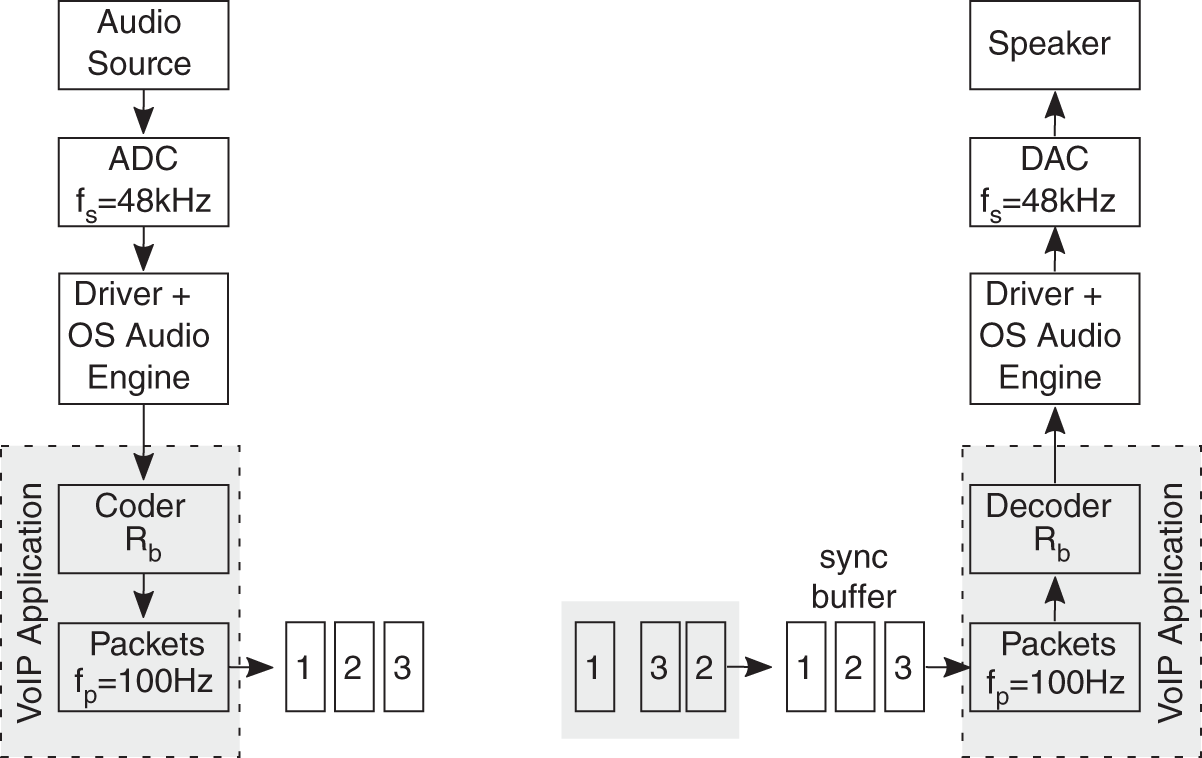
Figure 5.16 Audio over IP.
5.3 Two‐channel Systems
Most two‐channel systems for stereo processing can be realized with one DSP connected via serial interfacing to ADCs and DACs, and some control logic for parameter adjustment. Figure 5.17 gives an overview. For further functionalities (such as USB, HDMI, LAN, WLAN), system on a chip (SoC) devices offer DSP computation and extended communication interfaces.
5.4 Multi‐channel Systems
Multi‐channel systems can be realized by parallel DSP processing of multiple audio channels using multicore CPUs, GPUs, and FPGAs (field programmable gate arrays). A mixing console with ![]() input and
input and ![]() output channels, such as depicted in Fig. 5.18, can be realized by a single FPGA and adapted audio interface to ADCs/DACs/AES‐EBU/MADI devices and of course standard computer interfaces such as X Gbit/s USB or Ethernet.
output channels, such as depicted in Fig. 5.18, can be realized by a single FPGA and adapted audio interface to ADCs/DACs/AES‐EBU/MADI devices and of course standard computer interfaces such as X Gbit/s USB or Ethernet.

Figure 5.17 Two‐channel DSP system with two‐channel AD/DA converters (C = control, A = address, D = data, SDATA = serial data, SCLK = bit clock, WCLK = word clock, SDRX = serial input, SDTX = serial output).

Figure 5.18 Mixing console application of a multichannel system.
References
- [AES3] AES3‐2009: AES Recommended Practice for Digital Audio Engineering – Serial Transmission Format for Two‐Channel Linearly Represented Digital Audio.
- [AES10] AES10‐2020: AES Recommended Practice for Digital Audio Engineering – Serial Multichannel Audio Digital Interface (MADI).
- [AES50] AES50‐2011: AES standard for digital audio engineering – High‐resolution multi‐channel audio interconnection (HRMAI).
- [AES67] AES67‐2018: AES standard for audio applications of networks – High‐performance streaming audio‐over‐IP interoperability.