Chapter 6
Equalizers
U. Zölzer
Spectral sound equalization is one of the most important methods for processing audio signals. Equalizers are found in various forms in the transmission of audio signals from a sound studio to the listener. The more complex filter functions are used in sound studios. However, in almost every consumer product like car radios, hi‐fi amplifiers etc., simple filter functions are used for sound equalization. We first discuss basic filter types followed by the design and implementation of recursive audio filters. In the third and fourth sections, linear‐phase non‐recursive filter structures and their implementation are introduced.
6.1 Basics
For filtering of audio signals, the following filter types are used.
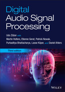
- Lowpass and highpass filters with cutoff frequency
 (3 dB cutoff frequency) are shown with their magnitude response in Fig. 6.1. They have a passband in the lower and higher frequency range, respectively.
 - Bandpass and bandstop filters (magnitude responses in Fig. 6.1) have a center frequency
 and a lower and upper
  and
and  cutoff frequency. They have a pass‐ and stopband in the middle of the frequency range. For the bandwidth of a bandpass or a bandstop filter, we have
(6.1)
cutoff frequency. They have a pass‐ and stopband in the middle of the frequency range. For the bandwidth of a bandpass or a bandstop filter, we have
(6.1)
Bandpass filters with a constant relative bandwidth
 are very important for audio applications [Cre03]. The bandwidth is proportional to the center frequency, which is given by
  (see Fig. 6.2).
Figure 6.1 Linear magnitude responses of lowpass, highpass, bandpass, and bandstop filters.
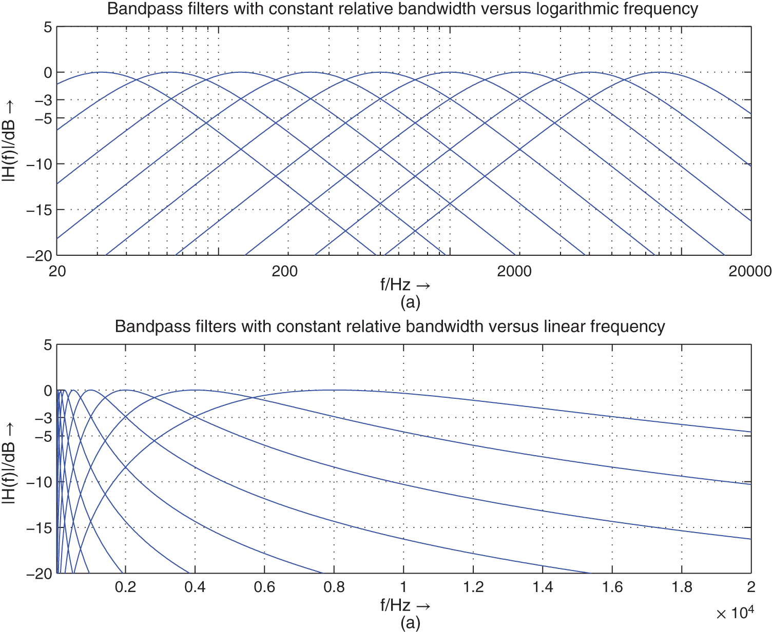
Figure 6.2 Logarithmic magnitude responses of bandpass filters with constant relative bandwidth.
- Octave filters are bandpass filters with special cutoff frequencies given by
(6.2)
 (6.3)
(6.3)
A spectral decomposition of the audio frequency range with octave filters is shown in Fig. 6.3. At the lower and upper cutoff frequency, an attenuation of
 dB occurs. The upper octave band is represented as a highpass. A parallel connection of octave filters can be used for a spectral analysis of the audio signal in octave frequency bands. This decomposition is used for the signal power distribution across the octave bands. For the center frequencies of octave bands, we get
 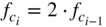 . The weighting of octave bands with gain factors
  and summation of the weighted octave bands represents an octave equalizer for sound processing (see Fig. 6.4). For this application, the lower and upper cutoff frequencies need an attenuation of
  dB, such that a sinusoid at the crossover frequency has gain of 0 dB. The attenuation of
  dB is achieved through a series connection of two octave filters with
  dB attenuation.
Figure 6.3 Linear magnitude responses of octave filters and decomposition of an octave band by three one‐third octave filters.
- One‐third octave filters are bandpass filters (see Fig. 6.3) with cutoff frequencies given by
(6.4)
 (6.5)
(6.5)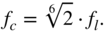
The attenuation at the lower and upper cutoff frequency is
 dB. One‐third octave filters split an octave into three frequency bands (see Fig. 6.3).
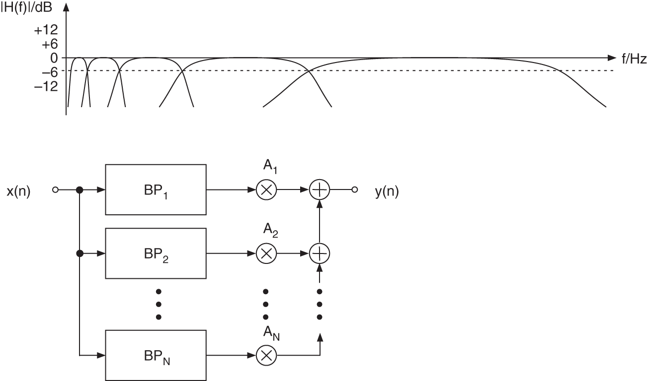
Figure 6.4 Parallel connection of bandpass filters (BP) for octave/one‐third octave equalizers with gain factors (
 for octave or one‐third octave band).
 - Shelving filters and peak filters are special weighting filters, which are based on lowpass/highpass/bandpass filters and a direct path (see Section 6.2.2). They have no stopband compared with lowpass/highpass/bandpass filters. They are used in a series connection of shelving and peak filters, as shown in Fig. 6.5. The lower frequency range is equalized by lowpass shelving filters and the higher frequencies are modified by highpass shelving filters. Both filter types allow the adjustment of the cutoff frequency and gain factor. For the mid‐frequency range, a series connection of peak filters with variable center frequency, bandwidth, and gain factor are used. These shelving and peak filters can also be applied for octave and one‐third octave equalizers in a series connection.

Figure 6.5 Series connection of shelving and peak filters (low‐frequency LF, high‐frequency HF).
- Weighting filters are used for signal level and noise measurement applications. The signal from a device under test is first passed through the weighting filter and then a root‐mean‐square or peak value measurement is performed. The two most commonly used filters are the A‐weighting filter and the CCIR‐468 weighting filter (see Fig. 6.6). Both weighting filters take the increased sensitivity of human perception in the 1–6 kHz frequency range into account. The 0 dB of the magnitude response of both filters is crossed at 1 kHz. The CCIR‐468 weighting filter has a gain of 12 dB at 6 kHz. A variant of the CCIR‐468 filter is the ITU‐ARM 2‐kHz weighting filter, which is a 5.6‐dB down‐tilted version of the CCIR‐468 filters and passes 0 dB at 2 kHz.
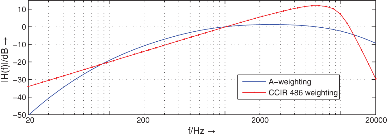
Figure 6.6 Magnitude responses of weighting filters for root‐mean‐square and peak value measurements.
6.2 Recursive Audio Filters
6.2.1 Design
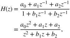
A certain filter response can be approximated by two kinds of transfer function. On the one hand, the combination of poles and zeros leads to a very low‐order transfer function ![]() in fractional form, which solves the given approximation problem. The digital implementation of this transfer function needs recursive procedures owing to its poles. On the other hand, the approximation problem can be solved by placing only zeros in the
in fractional form, which solves the given approximation problem. The digital implementation of this transfer function needs recursive procedures owing to its poles. On the other hand, the approximation problem can be solved by placing only zeros in the ![]() ‐plane. This transfer function
‐plane. This transfer function ![]() has, in addition to its zeros, a corresponding number of poles at the origin of the
has, in addition to its zeros, a corresponding number of poles at the origin of the ![]() ‐plane. The order of this transfer function, for the same approximation conditions, is substantially higher than for transfer functions consisting of poles and zeros. In view of an economical implementation of a filter algorithm in terms of complexity, recursive filters achieve shorter computing time owing to their lower order. For a sampling rate of 48 kHz, the algorithm has
‐plane. The order of this transfer function, for the same approximation conditions, is substantially higher than for transfer functions consisting of poles and zeros. In view of an economical implementation of a filter algorithm in terms of complexity, recursive filters achieve shorter computing time owing to their lower order. For a sampling rate of 48 kHz, the algorithm has ![]() of processing time available. With the digital signal processors (DSPs) presently available, it is easily possible to implement recursive digital filters for audio applications within this sampling period using only one DSP. To design the typical audio equalizers, we will start with filter designs in the S‐domain. These filters will then be mapped to the Z‐domain by the bilinear transformation.
of processing time available. With the digital signal processors (DSPs) presently available, it is easily possible to implement recursive digital filters for audio applications within this sampling period using only one DSP. To design the typical audio equalizers, we will start with filter designs in the S‐domain. These filters will then be mapped to the Z‐domain by the bilinear transformation.
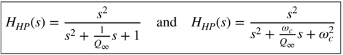
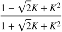
Lowpass/Highpass Filters. To limit the audio spectrum, lowpass and highpass filters with Butterworth response are used in analog mixers. They offer a monotonic passband and a monotonically decreasing stopband attenuation per octave (![]() dB/oct.) that is determined by the filter order. Lowpass filters of the second and fourth order are commonly used. The normalized and denormalized second‐order lowpass transfer functions are given by
dB/oct.) that is determined by the filter order. Lowpass filters of the second and fourth order are commonly used. The normalized and denormalized second‐order lowpass transfer functions are given by

where ![]() is the cutoff frequency and
is the cutoff frequency and ![]() is the pole quality factor. The
is the pole quality factor. The ![]() ‐factor
‐factor ![]() of a Butterworth approximation is equal to 1/
of a Butterworth approximation is equal to 1/![]() . The denormalization of a transfer function is obtained by replacing the Laplace variable
. The denormalization of a transfer function is obtained by replacing the Laplace variable ![]() by
by ![]() in the normalized transfer function.
in the normalized transfer function.
The corresponding second‐order highpass transfer functions
are obtained by a lowpass to highpass transformation. Figure 6.7 shows the pole‐zero locations in the s‐plane. The amplitude frequency response of a highpass filter with a 3‐dB cutoff frequency of 50 Hz and a lowpass filter with a 3‐dB cutoff frequency of 5000 Hz are shown in Fig. 6.8. Second‐ and fourth‐order filters are shown.
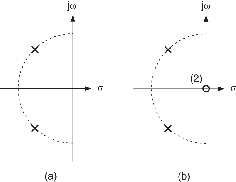
Figure 6.7 Pole‐zero location for (a) second‐order lowpass and (b) second‐order highpass.

Figure 6.8 Frequency response of lowpass and highpass filters – highpass  = 50 Hz (second/fourth order), lowpass
  = 5000 Hz (second/fourth order).
Table 6.1 summarizes the transfer functions of lowpass and highpass filters with Butterworth response.
Table 6.1 Transfer functions of lowpass and highpass filters.
| Lowpass | 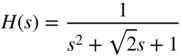 | second order |
 | fourth order | |
| Highpass |  | second order |
 | fourth order |
Bandpass and bandstop filters. The normalized and denormalized bandpass transfer functions of second order are

and the bandstop transfer functions are given by
The relative bandwidth can be expressed by the ![]() ‐factor
‐factor

which is the ratio of center frequency ![]() and the 3‐dB bandwidth given by
and the 3‐dB bandwidth given by ![]() . The magnitude responses of bandpass filters with constant relative bandwidth are shown in Fig. 6.2. Such kinds of filters are also called constant‐Q filters. The geometric symmetric behavior of the frequency response regarding the center frequency
. The magnitude responses of bandpass filters with constant relative bandwidth are shown in Fig. 6.2. Such kinds of filters are also called constant‐Q filters. The geometric symmetric behavior of the frequency response regarding the center frequency ![]() is clearly noticeable (symmetry regarding the center frequency using a logarithmic frequency axis).
is clearly noticeable (symmetry regarding the center frequency using a logarithmic frequency axis).
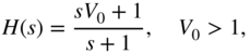
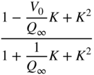
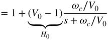
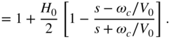
Shelving Filters. In addition to the purely band‐limiting filters like lowpass and highpass filters, shelving filters are used to perform weighting of certain frequencies. A simple approach for a first‐order lowpass shelving filter is given by
It consists of a first‐order lowpass filter with dc amplification of ![]() connected in parallel with an allpass system of transfer function equal to 1. Equation (6.11) can be written as
connected in parallel with an allpass system of transfer function equal to 1. Equation (6.11) can be written as

where ![]() determines the amplification at
determines the amplification at ![]() . By changing the parameter
. By changing the parameter ![]() , any desired boost (
, any desired boost (![]() ) and cut (
) and cut (![]() ) level can be adjusted. Figure 6.9 shows the frequency responses for
) level can be adjusted. Figure 6.9 shows the frequency responses for ![]() Hz. For
Hz. For ![]() , the cutoff frequency is dependent on
, the cutoff frequency is dependent on ![]() and is moved toward lower frequencies.
and is moved toward lower frequencies.

Figure 6.9 Frequency response of transfer function (6.12) with varying  and cutoff frequency
  Hz.
Hz.
To obtain a symmetrical frequency response with respect to the zero‐decibel line without changing the cutoff frequency, it is necessary to invert the transfer function (6.12) in the case of cut (![]() ). This has the effect of swapping poles with zeros and leads to the transfer function
). This has the effect of swapping poles with zeros and leads to the transfer function

for the cut case. Figure 6.10 shows the corresponding frequency responses for varying ![]() .
.
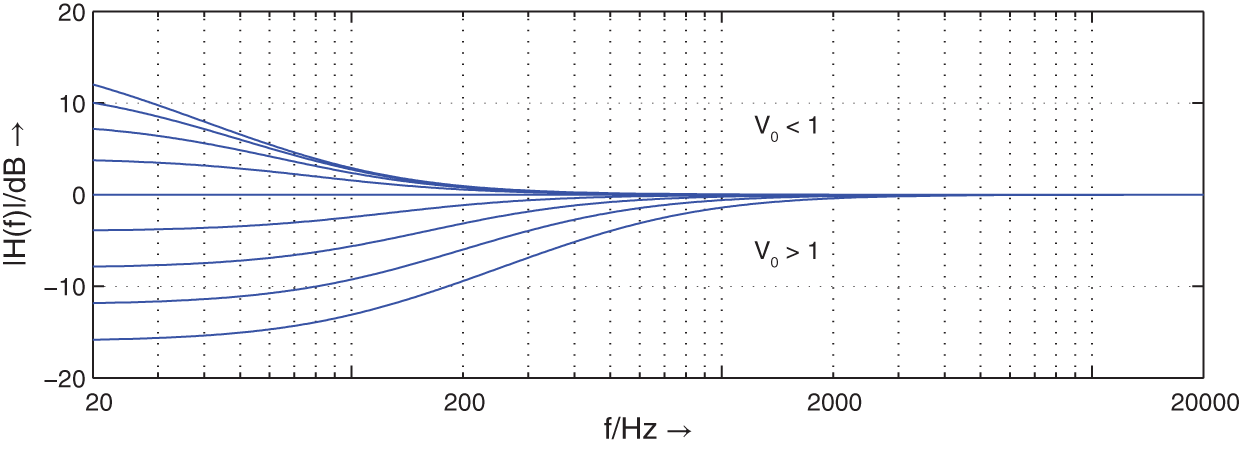
Figure 6.10 Frequency responses of transfer function (6.13) with varying  and cutoff frequency
  Hz.
Hz.
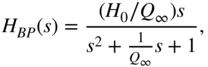
Finally, Figure 6.11 shows the locations of poles and zeros for both the boost and the cut cases. By moving zeros and poles on the negative ![]() ‐axis, boost and cut can be adjusted.
‐axis, boost and cut can be adjusted.

Figure 6.11 Pole‐zero locations of a first‐order low‐frequency shelving filter.
The equivalent shelving filter for high frequencies can be obtained by

which is a parallel connection of a first‐order highpass with gain ![]() and a system with transfer function equal to 1. In the case of boost, the transfer function can be written with
and a system with transfer function equal to 1. In the case of boost, the transfer function can be written with ![]() as
as
and for cut, we get

The parameter ![]() determines the value of the transfer function
determines the value of the transfer function ![]() at
at ![]() for high‐frequency shelving filters.
for high‐frequency shelving filters.
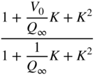
To increase the slope of the filter response in the transition band, a general second‐order transfer function
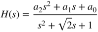
is considered, in which complex zeros are added to the complex poles. The calculation of poles leads to
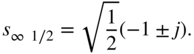
If the complex zeros
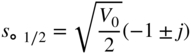
are moved on a straight line with the help of the parameter ![]() (see Fig. 6.12 ), the transfer function
(see Fig. 6.12 ), the transfer function

of a second‐order low‐frequency shelving filter is obtained. The parameter ![]() determines the boost for low frequencies. The cut case can be achieved by inversion of Eq. (6.20).
determines the boost for low frequencies. The cut case can be achieved by inversion of Eq. (6.20).

Figure 6.12 Pole‐zero locations of a second‐order low‐frequency shelving filter.
A lowpass to highpass transformation of Eq. (6.20) provides the transfer function

of a second‐order high‐frequency shelving filter. The zeros

are moved on a straight line toward the origin with increasing ![]() (see Fig. 6.13 ). The cut case is obtained by inverting the transfer function (6.21). Figure 6.14 shows the amplitude frequency response of a second‐order low‐frequency shelving filter with cutoff frequency 100 Hz and a second‐order high‐frequency shelving filter with cutoff frequency 5000 Hz (parameter
(see Fig. 6.13 ). The cut case is obtained by inverting the transfer function (6.21). Figure 6.14 shows the amplitude frequency response of a second‐order low‐frequency shelving filter with cutoff frequency 100 Hz and a second‐order high‐frequency shelving filter with cutoff frequency 5000 Hz (parameter ![]() ).
).

Figure 6.13 Pole‐zero locations of second‐order high‐frequency shelving filter.
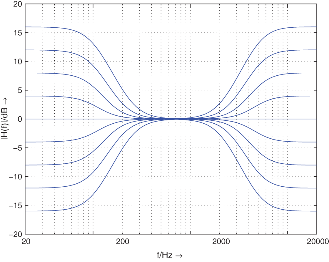
Figure 6.14 Frequency responses of second‐order low‐/high‐frequency shelving filters – low‐frequency shelving filter  = 100 Hz (parameter
  ), high‐frequency shelving filter
  = 5000 Hz (parameter
  ).
).
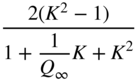
Peak Filter. Another equalizer used for boosting or cutting any desired frequency is the peak filter. A peak filter can be obtained by a parallel connection of a direct path and a bandpass according to
With the help of a second‐order bandpass transfer function
the transfer function

of a peak filter can be derived. It can be shown that the maximum of the amplitude frequency response at the center frequency is determined by the parameter ![]() . The relative bandwidth is fixed by the
. The relative bandwidth is fixed by the ![]() ‐factor. The geometrical symmetry of the frequency response relative to the center frequency remains constant for the transfer function of a peak filter given by Eq. (6.25). The poles and zeros lie on the unit circle. By adjusting the parameter
‐factor. The geometrical symmetry of the frequency response relative to the center frequency remains constant for the transfer function of a peak filter given by Eq. (6.25). The poles and zeros lie on the unit circle. By adjusting the parameter ![]() , the complex zeros are moved with respect to the complex poles. Figure 6.15 shows this for the boost and cut cases. With increasing
, the complex zeros are moved with respect to the complex poles. Figure 6.15 shows this for the boost and cut cases. With increasing ![]() ‐factor, the complex poles move toward the
‐factor, the complex poles move toward the ![]() ‐axis on the unit circle.
‐axis on the unit circle.
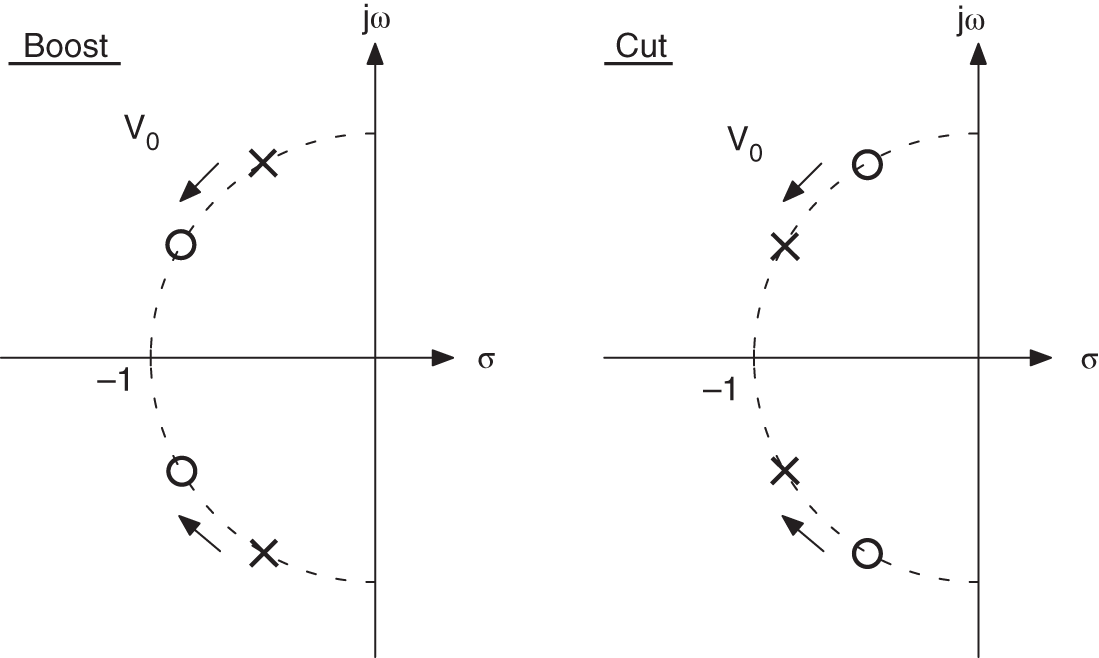
Figure 6.15 Pole‐zero locations of a second‐order peak filter.
Figure 6.16 shows the amplitude frequency response of a peak filter by changing the parameter ![]() at a center frequency of 500 Hz and a
at a center frequency of 500 Hz and a ![]() ‐factor of 1.25. Figure 6.17 shows the variation of the
‐factor of 1.25. Figure 6.17 shows the variation of the ![]() ‐factor
‐factor ![]() at a center frequency of 500 Hz, a boost/cut of
at a center frequency of 500 Hz, a boost/cut of ![]() dB, and
dB, and ![]() ‐factor of 1.25. Finally, the variation of the center frequency with boost and cut of
‐factor of 1.25. Finally, the variation of the center frequency with boost and cut of ![]() dB and a
dB and a ![]() ‐factor 1.25 is shown in Fig. 6.18 .
‐factor 1.25 is shown in Fig. 6.18 .
Figure 6.16 Frequency response of a peak filter –  = 500 Hz,
  = 1.25, cut parameter
  .
.

Figure 6.17 Frequency responses of peak filters –  = 500 Hz, boost/cut
  dB,
dB,  = 0.707, 1.25, 2.5, 3, 5.
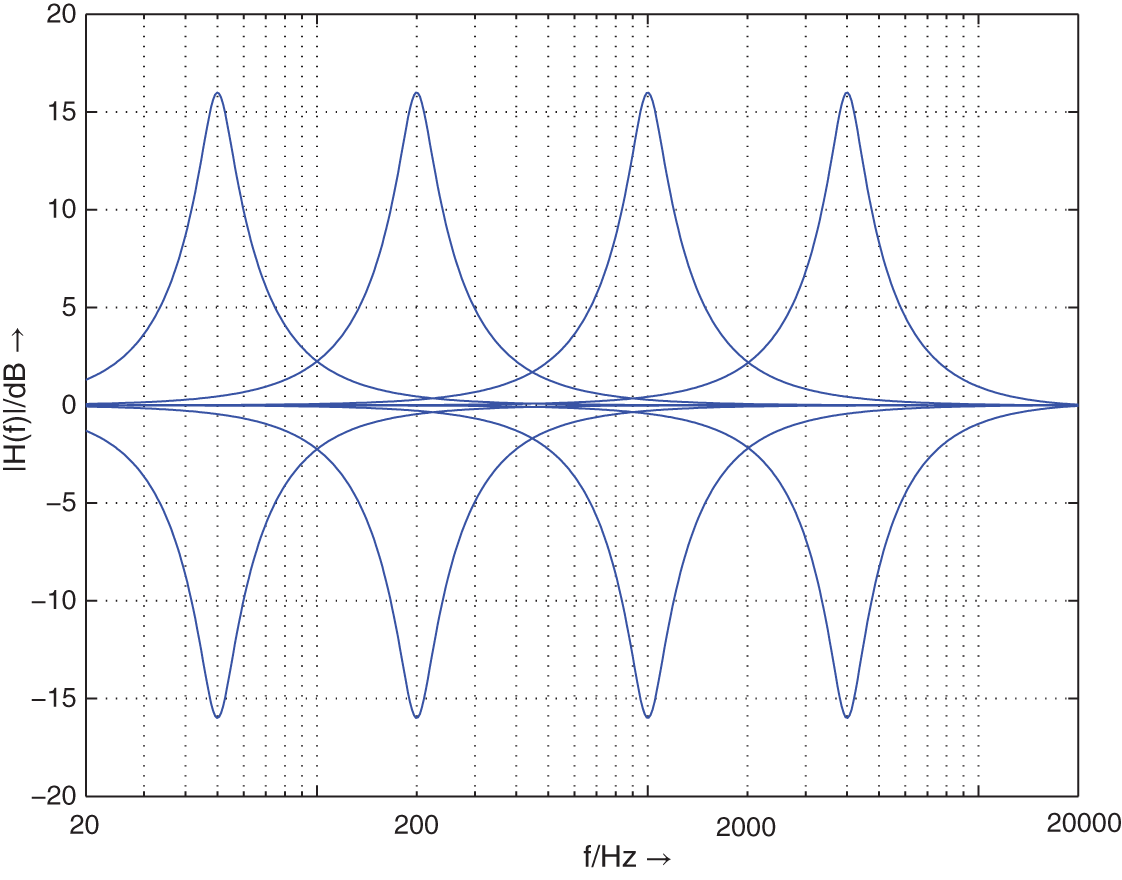
Figure 6.18 Frequency responses of peak filters – boost/cut  dB,
dB,  = 1.25,
  = 50, 200, 1000, 4000 Hz.
Mapping to Z‐domain. To implement a digital filter, the filter designed in the S‐domain with transfer function ![]() is converted to the Z‐domain with the help of a suitable transformation to obtain the transfer function
is converted to the Z‐domain with the help of a suitable transformation to obtain the transfer function ![]() . The impulse‐invariant transformation is not suitable as it leads to overlapping effects if the transfer function
. The impulse‐invariant transformation is not suitable as it leads to overlapping effects if the transfer function ![]() is not band limited to half the sampling rate. An independent mapping of poles and zeros from the S‐domain into poles and zeros in the Z‐domain is possible with help of the bilinear transformation given by
is not band limited to half the sampling rate. An independent mapping of poles and zeros from the S‐domain into poles and zeros in the Z‐domain is possible with help of the bilinear transformation given by
Tables 6.2 , 6.3 , 6.4 , and 6.5 contain the coefficients of the second‐order transfer function

which are determined by the bilinear transformation and the auxiliary variable ![]() for all discussed audio filter types. Further filter designs of peak and shelving filters are discussed in [Moo83, Whi86, Sha92, Bri94, Orf96a, Dat97, Cla00, Väl16]. A method for reducing the warping effect of the bilinear transform is proposed in [Orf96b]. Strategies for time‐variant switching of audio filters can be found in [Rab88, Mou90, Zöl93, Din95, Väl98].
for all discussed audio filter types. Further filter designs of peak and shelving filters are discussed in [Moo83, Whi86, Sha92, Bri94, Orf96a, Dat97, Cla00, Väl16]. A method for reducing the warping effect of the bilinear transform is proposed in [Orf96b]. Strategies for time‐variant switching of audio filters can be found in [Rab88, Mou90, Zöl93, Din95, Väl98].
Table 6.2 Lowpass/highpass/bandpass filter design.
| Lowpass (second‐order) | ||||
 |  |  |  |  |
| Highpass (second‐order) | ||||
 |  |  |  |  |
| Bandpass (second‐order) | ||||
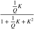 |  |  | 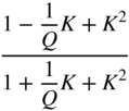 | |
Table 6.3 Peak filter design with gain ![]() in dB.
in dB.
| Peak (boost | ||||
 |  |  |  |  |
| Peak (cut | ||||
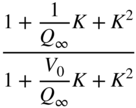 | 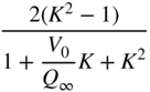 | 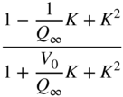 |  | 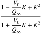 |
Table 6.4 Low‐frequency shelving filter design with gain ![]() in dB.
in dB.
| Low‐frequency shelving (Boost | ||||
| | | | | |
 |  |  |  |  |
| Low‐frequency shelving (Cut | ||||
| | | | | |
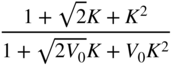 |  | 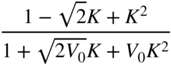 |  |  |
Table 6.5 High‐frequency shelving filter design with gain ![]() in dB.
in dB.
| High‐frequency shelving (Boost | ||||
| | | | | |
 |  |  |  |  |
| High‐frequency shelving (Cut | ||||
| | | | | |
 |  |  |  |  |
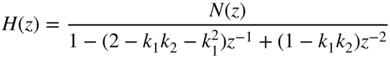
6.2.2 Parametric Filter Structures
Parametric filter structures allow direct access to the parameters of the transfer function, like center/cutoff frequency, bandwidth, and gain, through the control of associated coefficients. To modify one of these parameters, it is therefore not necessary to compute a complete set of coefficients for a second‐order transfer function, but instead only one coefficient in the filter structure is calculated.
An independent control of gain, cutoff/center frequency, and bandwidth for shelving and peak filters is achieved by a feed‐forward (FF) structure for boost and a feed‐backward (FB) structure for cut, as shown in Fig. 6.19 . The corresponding transfer functions are

The boost/cut factor is ![]() . For digital filter implementations, it is necessary for the FB case that the inner transfer function be of the form
. For digital filter implementations, it is necessary for the FB case that the inner transfer function be of the form ![]() to ensure causality. A parametric filter structure proposed by Harris [Har93] is based on the FF/FB technique, but the frequency response shows slight deviations near
to ensure causality. A parametric filter structure proposed by Harris [Har93] is based on the FF/FB technique, but the frequency response shows slight deviations near ![]() and
and ![]() from the desired one. This arises from the
from the desired one. This arises from the ![]() in the FF/FB branch. Delay‐free loops inside filter computations can be solved by the methods presented in [Här98, Fon01, Fon03]. Higher‐order parametric filter designs have been introduced in [Kei04, Orf05, Hol06a, Hol06b, Hol06c, Hol06d]. It is possible to implement typical audio filters with only an FF structure. The complete decoupling of the control parameters is possible for the boost case, but there remains a coupling between bandwidth and gain factor for the cut case. In the following, two approaches for parametric audio filter structures based on an allpass decomposition of the transfer function will be discussed.
in the FF/FB branch. Delay‐free loops inside filter computations can be solved by the methods presented in [Här98, Fon01, Fon03]. Higher‐order parametric filter designs have been introduced in [Kei04, Orf05, Hol06a, Hol06b, Hol06c, Hol06d]. It is possible to implement typical audio filters with only an FF structure. The complete decoupling of the control parameters is possible for the boost case, but there remains a coupling between bandwidth and gain factor for the cut case. In the following, two approaches for parametric audio filter structures based on an allpass decomposition of the transfer function will be discussed.

Figure 6.19 Filter structure for implementing boost and cut filters.
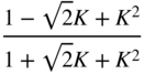
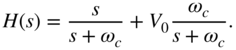
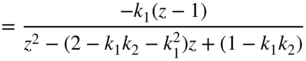
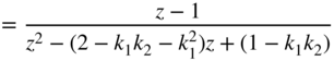
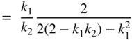
Regalia filter [Reg87]. The denormalized transfer function of a first‐order shelving filter is given by

with
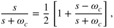
A decomposition of Eq. (6.30) leads to
The lowpass and highpass transfer functions in Eq. (6.31) can be expressed by an allpass decomposition of the form

With the allpass transfer function
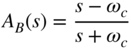
for boost, Eq. (6.30) can be rewritten as
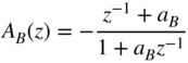
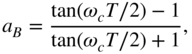
The bilinear transformation ![]() leads to
leads to
with
and the frequency parameter
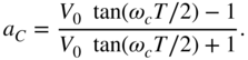
A filter structure for direct implementation of Eq. (6.36) is presented in Fig. 6.20 a. Other possible structures can be seen in Fig. 6.20 b,c. For the cut case ![]() , the cutoff frequency of the filter moves towards lower frequencies [Reg87].
, the cutoff frequency of the filter moves towards lower frequencies [Reg87].
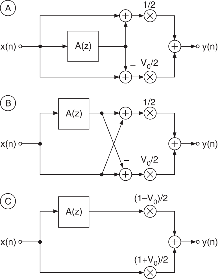
Figure 6.20 Filter structures by Regalia.
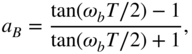
To retain the cutoff frequency for the cut case [Zöl95], the denormalized transfer function of a first‐order shelving filter (cut)

with the boundary conditions

can be decomposed as follows:

With the allpass decompositions

and the allpass transfer function
for cut, Eq. (6.39) can be rewritten as
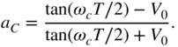
The bilinear transformation leads to
with

and the frequency parameter

Owing to (Eqs. 6.45) and (6.36), boost and cut can be implemented with the same filter structure (see Fig. 6.20 ). However, it has to be noted that the frequency parameter ![]() , as in Eq. (6.47) for cut, depends on the cutoff frequency and gain.
, as in Eq. (6.47) for cut, depends on the cutoff frequency and gain.
A second‐order peak filter is obtained by a lowpass to bandpass transformation according to

For an allpass, as given in (Eqs. 6.37) and (6.46), the second‐order allpass is given by
with parameters (cut as in [Zöl95])

The center frequency ![]() is fixed by the parameter
is fixed by the parameter ![]() , the bandwidth
, the bandwidth ![]() by the parameters
by the parameters ![]() and
and ![]() , and gain
, and gain ![]() by the parameter
by the parameter ![]() .
.
Simplified Allpass Decomposition [Zöl95]. The transfer function of a first‐order low‐frequency shelving filter can be a decomposed as


with
The transfer function (6.55) is composed of a direct branch and a lowpass filter. The first‐order lowpass filter is again implemented by an allpass decomposition. Applying the bilinear transformation to Eq. (6.55) leads to
with
For cut, the following decomposition can be derived:
The bilinear transformation applied to Eq. (6.63) again gives Eq. (6.59). The filter structure is identical for boost and cut. The frequency parameter ![]() for boost and
for boost and ![]() for cut can be calculated as
for cut can be calculated as
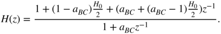
The transfer function of a first‐order low‐frequency shelving filter can be calculated as

With ![]() , the signal flow chart in Fig. 6.21 shows a first‐order lowpass filter and a first‐order low‐frequency shelving filter.
, the signal flow chart in Fig. 6.21 shows a first‐order lowpass filter and a first‐order low‐frequency shelving filter.

Figure 6.21 Low‐frequency shelving filter and first‐order lowpass filter.
The decomposition of a denormalized transfer function of a first‐order high‐frequency shelving filter can be given in the form of


where
The transfer function results by adding a highpass filter to a constant. Applying the bilinear transformation to Eq. (6.68) gives
with
For cut, the decomposition can be given by

which in return results in Eq. (6.71) after a bilinear transformation. The boost and cut parameters can be calculated as
The transfer function of a first‐order high‐frequency shelving filter can then be written as
With ![]() , the signal flow chart in Fig. 6.22 shows a first‐order highpass filter and a high‐frequency shelving filter.
, the signal flow chart in Fig. 6.22 shows a first‐order highpass filter and a high‐frequency shelving filter.

Figure 6.22 First‐order high‐frequency shelving and highpass filters.
The implementation of a second‐order peak filter can be carried out with a lowpass to bandpass transformation of a first‐order shelving filter. However, the addition of a second‐order bandpass filter to a constant branch also results in a peak filter. With the help of an allpass implementation of a bandpass filter, as given by
and

a second‐order peak filter can be expressed as
The bandwidth parameters ![]() and
and ![]() for boost and cut are given by
for boost and cut are given by

The center frequency parameter ![]() and the coefficient
and the coefficient ![]() are given by
are given by
The transfer function of a second‐order peak filter results in
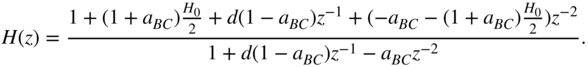
The signal flow charts for a second‐order peak filter and a second‐order bandpass filter are shown in Fig. 6.23 .

Figure 6.23 Second‐order peak filter and bandpass filter.

Figure 6.24 Low‐frequency first‐order shelving filter ( dB;
dB;  = 20, 50, 100, 1000 Hz).

Figure 6.25 First‐order high‐frequency shelving filter ( dB;
dB;  = 1, 3, 5, 10, 16 kHz).
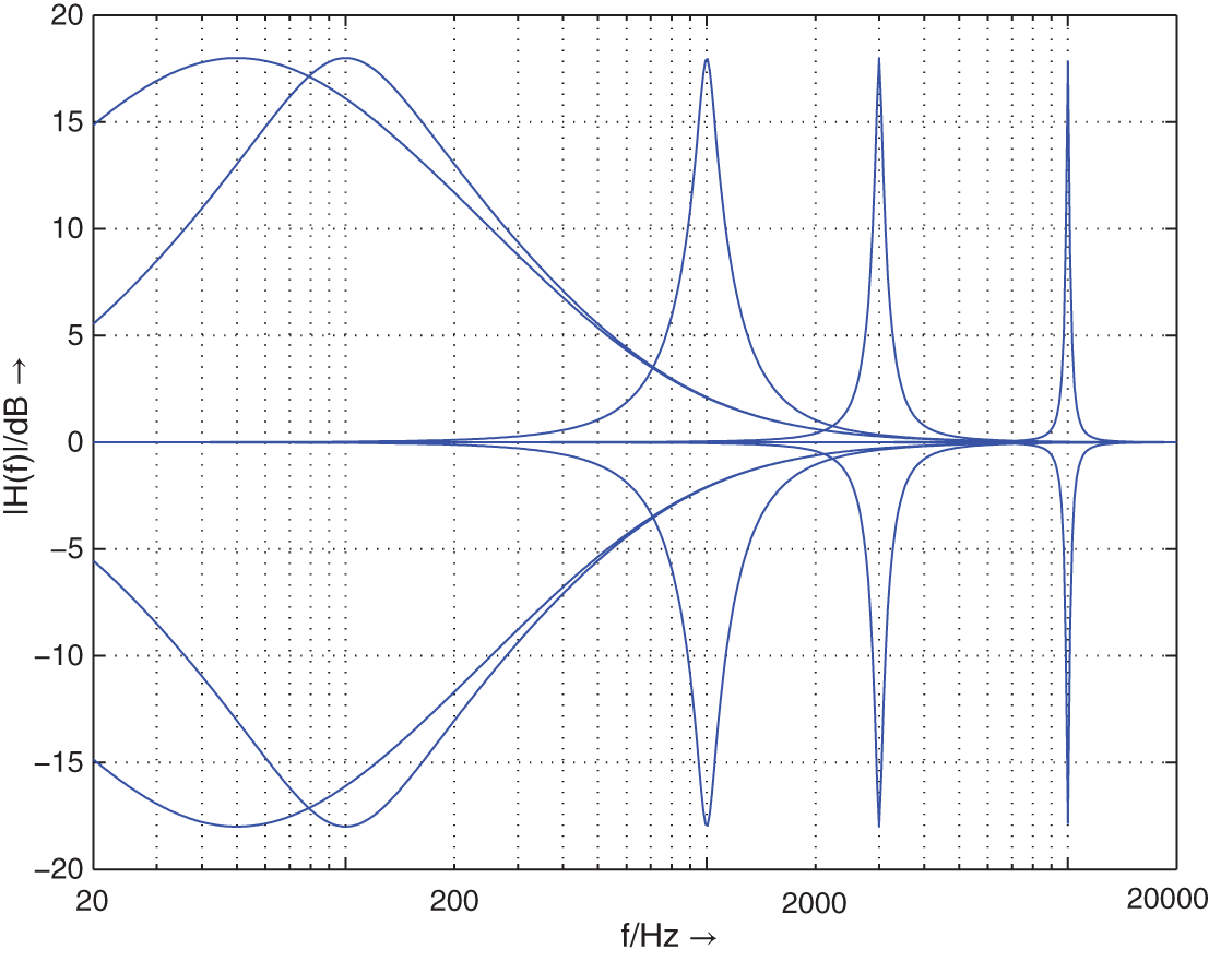
Figure 6.26 Second‐order peak filter ( dB;
dB;  = 50, 100, 1000, 3000, 10000 Hz;
  = 100 Hz).
The frequency responses for high‐frequency shelving, low‐frequency shelving, and peak filters are shown in Figs. 6.24 , 6.25 , and 6.26 .
6.2.3 Quantization Effects
The limited word length for digital recursive filters leads to two different types of quantization error. The quantization of the coefficients of a digital filter results in linear distortion which can be noticed as a deviation from the ideal frequency response. The quantization of the signal inside a filter structure is responsible for the maximum dynamic range and determines the noise behavior of the filter. Owing to rounding operations in a filter structure, round‐off noise is produced. Another effect of the signal quantization is limit cycles. They can be classified as overflow limit cycles, small‐scale limit cycles, and limit cycles correlated with the input signal. Limit cycles are very disturbing owing to their small‐band (sinusoidal) nature. The overflow limit cycles can be avoided by suitable scaling of the input signal. The effects of other errors mentioned above can be reduced by increasing the word lengths of the coefficient and the state variables of the filter structure.
The noise behavior and coefficient sensitivity of a filter structure depend on the topology and the cutoff frequency (position of the poles in the Z‐domain) of the filter. Because common audio filters operate between 20 Hz and 20 kHz at a sampling rate of 48 kHz, the filter structures are subjected to specially strict criteria with respect to error behavior. The frequency range for equalizers is between 20 Hz and 4–6 kHz because the human voice and many musical instruments have their formants in that frequency region. For given coefficient and signal word‐lengths (like in a digital signal processor), a filter structure with low round‐off noise for audio application can lead to a suitable solution. For this, the following second‐order filter structures are compared.
The basis of the following considerations is the relationship between the coefficient sensitivity and round‐off noise. This was first stated by Fettweis [Fet72]. By increasing the pole density in a certain region of the ![]() ‐plane, the coefficient sensitivity and the round‐off noise of the filter structure are reduced. Owing to these improvements, the coefficient word‐length as well as signal word‐length can be reduced. Work in designing digital filters with minimum word‐length for coefficients and state variables was first carried out by Avenhaus [Ave71].
‐plane, the coefficient sensitivity and the round‐off noise of the filter structure are reduced. Owing to these improvements, the coefficient word‐length as well as signal word‐length can be reduced. Work in designing digital filters with minimum word‐length for coefficients and state variables was first carried out by Avenhaus [Ave71].
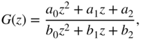
Typical audio filters like highpass/lowpass, peak/shelving filters can be described by the second‐order transfer function
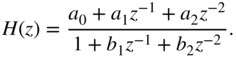
The recursive part of the difference equation, which can be derived from the transfer function (6.88), is considered more closely, because it plays a major role in affecting the error behavior. Owing to the quantization of the coefficients in the denominator in Eq. (6.88), the distribution of poles in the ![]() ‐plane is restricted (see Fig. 6.27 for 6‐bit quantization of coefficients). The pole distribution in the second quadrant of the
‐plane is restricted (see Fig. 6.27 for 6‐bit quantization of coefficients). The pole distribution in the second quadrant of the ![]() ‐plane is the mirror image of the first quadrant. Figure 6.28 shows a block diagram of the recursive part. Another equivalent representation of the denominator is given by
‐plane is the mirror image of the first quadrant. Figure 6.28 shows a block diagram of the recursive part. Another equivalent representation of the denominator is given by

Here ![]() is the radius and
is the radius and ![]() the corresponding phase of the complex poles. By quantizing these parameters, the pole distribution is altered in contrast to the case where
the corresponding phase of the complex poles. By quantizing these parameters, the pole distribution is altered in contrast to the case where ![]() and
and ![]() are quantized, as in Eq. (6.88).
are quantized, as in Eq. (6.88).

Figure 6.27 Direct‐form structure – pole distribution (6‐bit quantization).
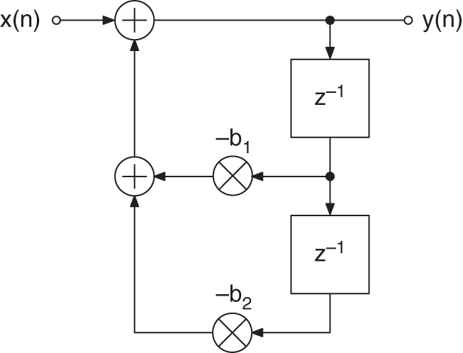
Figure 6.28 Direct‐form structure – block diagram of recursive part.
The state variable structure [Mul76, Bom85] is based on the approach by Gold and Rader [Gol67], which is given by

The possible pole locations are shown in Fig. 6.29 for 6‐bit quantization (block diagram of recursive part is shown in Fig. 6.30 ). Owing to the quantization of real and imaginary parts, a uniform grid of different pole locations results. In contrast to direct quantization of the coefficients ![]() and
and ![]() in the denominator, the quantization of the real and imaginary parts leads to an increase in the pole density at
in the denominator, the quantization of the real and imaginary parts leads to an increase in the pole density at ![]() . The possible pole locations in the second quadrant in the
. The possible pole locations in the second quadrant in the ![]() ‐plane are the mirror images of those in the first quadrant.
‐plane are the mirror images of those in the first quadrant.

Figure 6.29 Gold and Rader – pole distribution (6‐bit quantization).
Figure 6.30 Gold and Rader – block diagram of recursive part.
In [Kin72], a filter structure is suggested which has a pole distribution as shown in Fig. 6.31 (for the block diagram of recursive part, see Fig. 6.32 ).
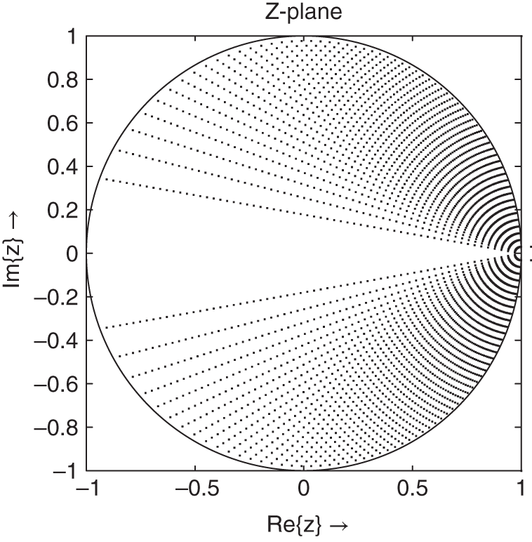
Figure 6.31 Kingsbury – pole distribution (6‐bit quantization).
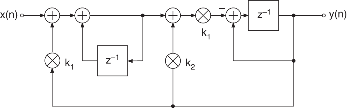
Figure 6.32 Kingsbury – block diagram of recursive part.
The corresponding transfer function
shows that in this case, the coefficients ![]() and
and ![]() can be obtained by a linear combination of the quantized coefficients
can be obtained by a linear combination of the quantized coefficients ![]() and
and ![]() . The distance
. The distance ![]() of the pole from the point
of the pole from the point ![]() determines the coefficients
determines the coefficients
as illustrated in Fig. 6.33 .
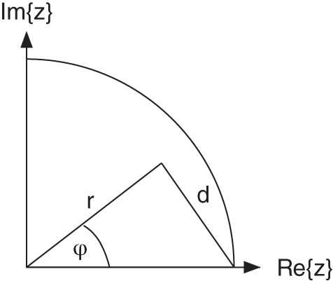
Figure 6.33 Geometric interpretation.
The filter structures under consideration show that by a suitable linear combination of quantized coefficients, any desired pole distribution can be obtained. An increase of the pole density at ![]() can be achieved by influencing the linear relationship between the coefficient
can be achieved by influencing the linear relationship between the coefficient ![]() and the distance
and the distance ![]() from
from ![]() [Zöl89, Zöl90]. The nonlinear relationship of the new coefficients gives the following structure with the transfer function
[Zöl89, Zöl90]. The nonlinear relationship of the new coefficients gives the following structure with the transfer function
and coefficients

with
The pole distribution of this structure is shown in Fig. 6.34 . The block diagram of the recursive part is illustrated in Fig. 6.35 . An increase in the pole density at ![]() in contrast to previous pole distributions is noticed. The pole distributions of the Kingsbury and Zölzer structures show a decrease in the pole density for higher frequencies. For the pole density, a symmetry with respect to the imaginary axis, as in the case of the direct‐form structure and the Gold and Rader structure, is not possible. However, changing the sign in the recursive part of the difference equation results in a mirror image of the pole density. The mirror image can be achieved through a change of sign in the denominator polynomial. The denominator polynomial
in contrast to previous pole distributions is noticed. The pole distributions of the Kingsbury and Zölzer structures show a decrease in the pole density for higher frequencies. For the pole density, a symmetry with respect to the imaginary axis, as in the case of the direct‐form structure and the Gold and Rader structure, is not possible. However, changing the sign in the recursive part of the difference equation results in a mirror image of the pole density. The mirror image can be achieved through a change of sign in the denominator polynomial. The denominator polynomial
shows that the real part depends on the coefficient of ![]() .
.
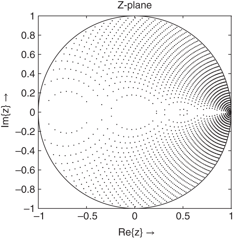
Figure 6.34 Zölzer – pole distribution (6‐bit quantization).

Figure 6.35 Zölzer – block diagram of recursive part.
Analytical Comparison of Noise Behavior of Different Filter Structures
In this section, recursive filter structures are analyzed in terms of their noise behavior in fixed‐point arithmetic [Zöl89, Zöl90, Zöl94]. The block diagrams provide the basis of an analytical calculation of noise power owing to the quantization of state variables. First of all, the general case is considered in which quantization is performed after multiplication. For this purpose, the transfer function ![]() of every multiplier output to the output of the filter structure is determined.
of every multiplier output to the output of the filter structure is determined.
For this error analysis, it is assumed that the signal within the filter structure covers the whole dynamic range so that the quantization error ![]() is not correlated with the signal. Consecutive quantization error samples are not correlated with each other so that a uniform power density spectrum results [Sri77]. It can also be assumed that different quantization errors
is not correlated with the signal. Consecutive quantization error samples are not correlated with each other so that a uniform power density spectrum results [Sri77]. It can also be assumed that different quantization errors ![]() are uncorrelated within the filter structure. Owing to the uniform distribution of the quantization error, the variance can be given by
are uncorrelated within the filter structure. Owing to the uniform distribution of the quantization error, the variance can be given by

The quantization error is added at every point of quantization and is filtered by the corresponding transfer function ![]() to the output of the filter. The variance of the output quantization noise (owing to the noise source
to the output of the filter. The variance of the output quantization noise (owing to the noise source ![]() ) is given by
) is given by

Exact solutions for the ring integral (6.100) can be found in [Jur64] for transfer functions up to the fourth order. With the ![]() norm of a periodic function
norm of a periodic function
the superposition of the noise variances leads with Eq. (6.101) to the total output noise variance
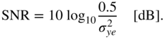
The signal‐to‐noise ratio (SNR) for a full‐range sinusoid can be written as
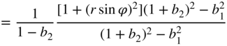
The ring integral
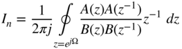
is given in [Jur64] for first‐order systems by

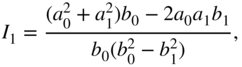
and for second‐order systems by
In the following, an analysis of the noise behavior for different recursive filter structures will be made. The noise transfer functions of individual recursive parts are responsible for noise shaping.
The error transfer function of a second‐order direct‐form structure (see Fig. 6.36 ) has only complex poles (see Table 6.6 ).

Figure 6.36 Direct form with additive error signal.
Table 6.6 Direct‐form – a) noise transfer function, b) quadratic ![]() norm, and c) output noise variance in the case of quantization after every multiplication.
norm, and c) output noise variance in the case of quantization after every multiplication.
| a) | 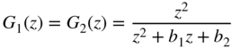 |
| b) |  |
| c) |  |
The implementation of poles near the unit circle leads to high amplification of the quantization error. The effect of the pole radius on the noise variance can be observed in the equation for output noise variance. The coefficient ![]() approaches 1 which leads to a huge increase in the output noise variance.
approaches 1 which leads to a huge increase in the output noise variance.
The Gold and Rader filter structure (Fig. 6.37 ) has an output noise variance that depends on the pole radius (see Table 6.7 ) and is independent of the pole phase. The latter fact is because of the uniform grid of the pole distribution. An additional zero on the real axis (![]() ) directly beneath the poles reduces the effect of the complex poles.
) directly beneath the poles reduces the effect of the complex poles.

Figure 6.37 Gold and Rader structure with additive error signals.
Table 6.7 Gold and Rader – a) noise transfer function, b) quadratic ![]() norm, and c) output noise variance in the case of quantization after every multiplication.
norm, and c) output noise variance in the case of quantization after every multiplication.
| a) | 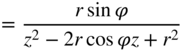 | |
| b) | 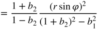 | |
 | ||
| c) | 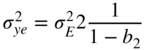 |
The Kingsbury filter (Fig. 6.38 and Table 6.8 ) and the Zölzer filter (Fig. 6.39 and Table 6.9 ), which is derived from it, show that the noise variance depends on the pole radius. The noise transfer functions have a zero at ![]() in addition to the complex poles. This zero reduces the amplifying effect of the pole near the unit circle at
in addition to the complex poles. This zero reduces the amplifying effect of the pole near the unit circle at ![]() .
.

Figure 6.38 Kingsbury structure with additive error signals.
Table 6.8 Kingsbury – a) noise transfer function, b) quadratic ![]() norm, and c) output noise variance in the case of quantization after every multiplication.
norm, and c) output noise variance in the case of quantization after every multiplication.
| a) |  | |
 | ||
 | ||
| b) | 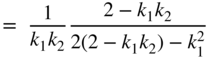 | |
 | ||
 | ||
| c) |  | |

Figure 6.39 Zölzer structure with additive error signals.
Table 6.9 Zölzer – a) noise transfer function, b) quadratic ![]() norm, and c) output noise variance in the case of quantization after every multiplication.
norm, and c) output noise variance in the case of quantization after every multiplication.
| a) |  | |
 | ||
 | ||
| b) |  | |
 | ||
 | ||
| c) | 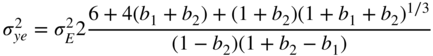 | |
Figure 6.40 shows the SNR versus the cutoff frequency for the four filter structures presented above. The signals are quantized to 16 bit. Here, the poles move with increasing cutoff frequency on the curve characterized by the ![]() ‐factor
‐factor ![]() in the
in the ![]() ‐plane. For very small cutoff frequencies, the Zölzer filter shows an improvement of 3 dB in terms of SNR compared with the Kingsbury filter and an improvement of 6 dB compared with the Gold and Rader filter. Up to 5 kHz, the Zölzer filter yields better results (see Fig. 6.41 ). From 6 kHz onwards, the reduction of pole density in this filter leads to a decrease in the SNR (see Fig. 6.41 ).
‐plane. For very small cutoff frequencies, the Zölzer filter shows an improvement of 3 dB in terms of SNR compared with the Kingsbury filter and an improvement of 6 dB compared with the Gold and Rader filter. Up to 5 kHz, the Zölzer filter yields better results (see Fig. 6.41 ). From 6 kHz onwards, the reduction of pole density in this filter leads to a decrease in the SNR (see Fig. 6.41 ).
With regard to the implementation of the these filters with digital signal processors, a quantization after every multiplication is not necessary. Quantization takes place when the accumulator has to be stored to memory. This can be seen in Figs. 6.42 , 6.43 , 6.44 , and 6.45 by introducing quantizers where they really occur. The resulting output noise variances are also shown. The SNR is plotted versus the cutoff frequency in Figs. 6.46 and 6.47 . In the case of direct‐form and Gold and Rader filters, the SNR increases by 3 dB whereas the output noise variance for the Kingsbury filter remains unchanged. The Kingsbury filter and the Gold and Rader filters exhibit similar results up to a frequency of 200 kHz (see Fig. 6.46 ). The Zölzer filter demonstrates an improvement of 3 dB compared with these structures. For frequencies of up to 2 kHz (see Fig. 6.47 ), it is seen that the increased pole density leads to an improvement of the SNR as well as a reduced effect owing to coefficient quantization.

Figure 6.40 SNR versus cutoff frequency – quantization of products ( Hz).
Hz).
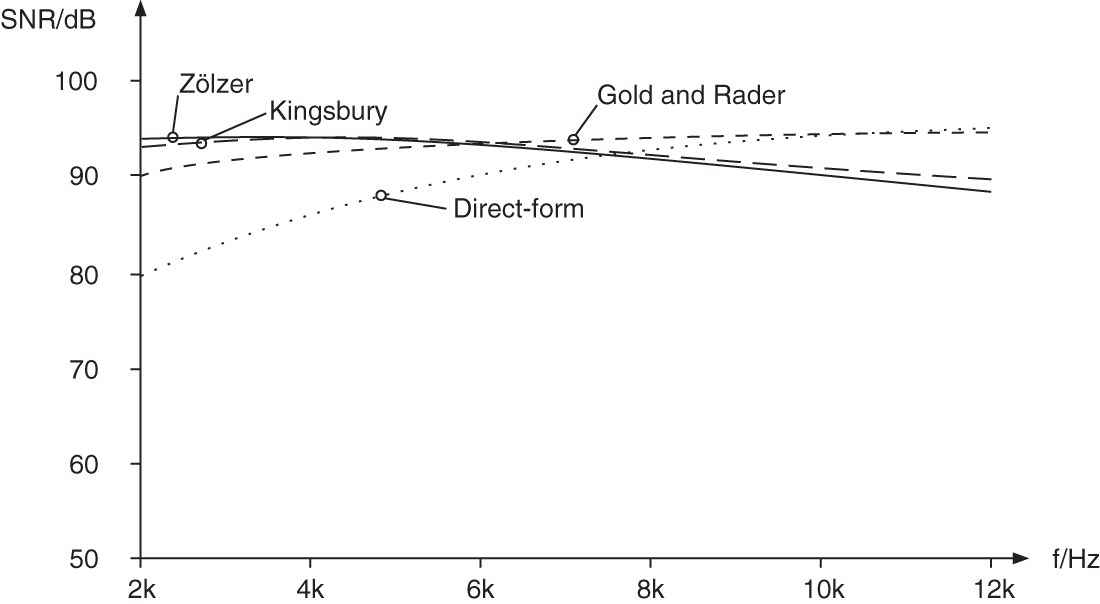
Figure 6.41 SNR versus cutoff frequency – quantization of products ( kHz).
kHz).

Figure 6.42 Direct‐form filter – quantization after accumulator.
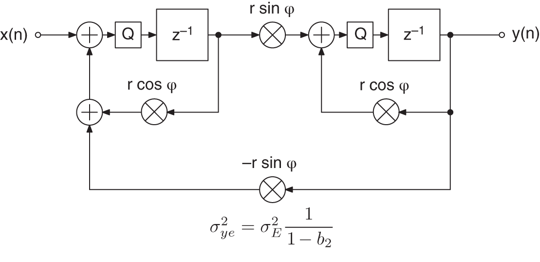
Figure 6.43 Gold and Rader filter – quantization after accumulator.
Figure 6.44 Kingsbury filter – quantization after accumulator.
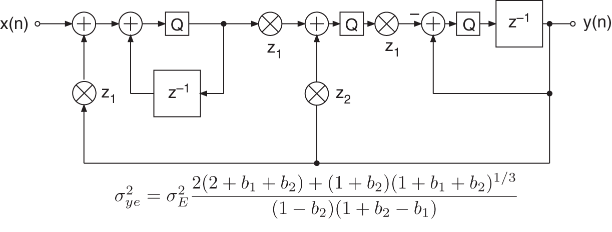
Figure 6.45 Zölzer filter – quantization after accumulator.
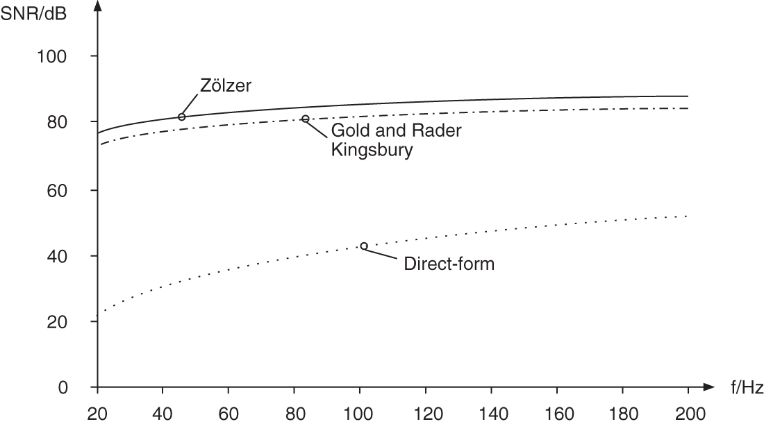
Figure 6.46 SNR versus cutoff frequency – quantization after accumulator ( Hz).
Hz).
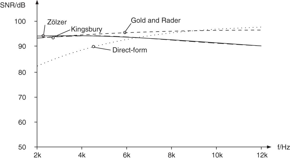
Figure 6.47 SNR versus cutoff frequency – quantization after accumulator ( kHz).
kHz).
Noise Shaping in Recursive Filters
The analysis of the noise transfer function of different structures shows that for three structures with low round‐off noise, a zero at ![]() occurs in the transfer functions
occurs in the transfer functions ![]() of the error signals in addition to the complex poles. This zero near the poles reduces the amplifying effect of the pole. If it is now possible to introduce another zero into the noise transfer function, then the effect of the poles is compensated for to a larger extent. The procedure of feeding back the quantization error, as shown in Chapter 2, produces an additional zero in the noise transfer function [Tra77, Cha78, Abu79, Bar82, Zöl89]. The feedback of the quantization error is first demonstrated with the help of the direct‐form structure, as shown in Fig. 6.48 . This generates a zero at
of the error signals in addition to the complex poles. This zero near the poles reduces the amplifying effect of the pole. If it is now possible to introduce another zero into the noise transfer function, then the effect of the poles is compensated for to a larger extent. The procedure of feeding back the quantization error, as shown in Chapter 2, produces an additional zero in the noise transfer function [Tra77, Cha78, Abu79, Bar82, Zöl89]. The feedback of the quantization error is first demonstrated with the help of the direct‐form structure, as shown in Fig. 6.48 . This generates a zero at ![]() in the noise transfer function given by
in the noise transfer function given by
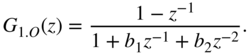
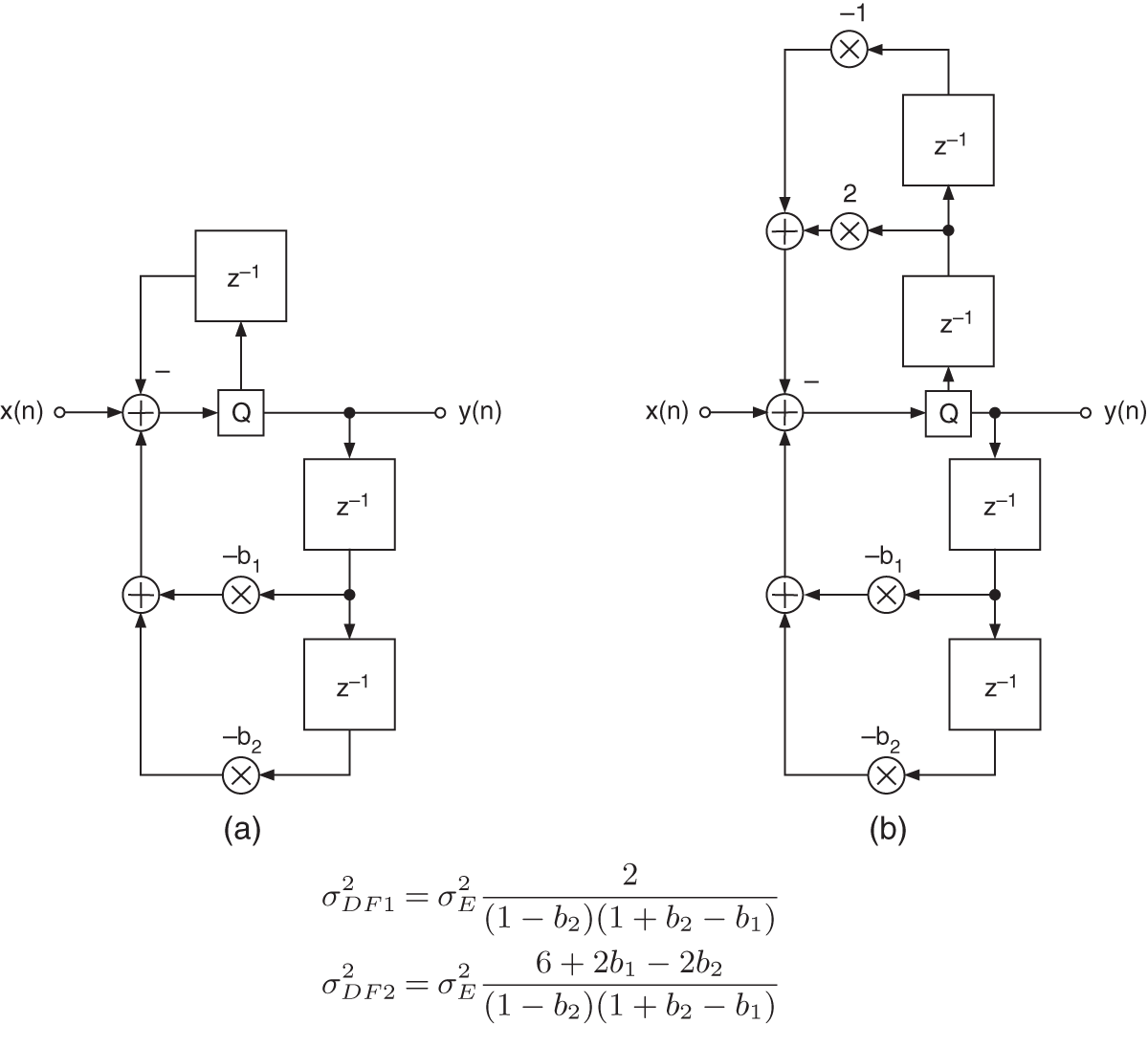
Figure 6.48 Direct‐form with noise shaping.
The resulting variance ![]() of the quantization error at the output of the filter is presented in Fig. 6.48 . To produce two zeros at
of the quantization error at the output of the filter is presented in Fig. 6.48 . To produce two zeros at ![]() , the quantization error is fed back over two delays weighted with 2 and
, the quantization error is fed back over two delays weighted with 2 and ![]() (see Fig. 6.48 b). The noise transfer function is, hence, given by
(see Fig. 6.48 b). The noise transfer function is, hence, given by
The SNR of the direct form is plotted versus the cutoff frequency in Fig. 6.49 . Even a single zero significantly improves the SNR in the direct form. The coefficients ![]() and
and ![]() approach
approach ![]() and 1, respectively, with the decrease of the cutoff frequency. With this, the error is filtered with a second‐order highpass. The introduction of the additional zeros in the noise transfer function only affects the noise signal of the filter. The input signal is only affected by the transfer function
and 1, respectively, with the decrease of the cutoff frequency. With this, the error is filtered with a second‐order highpass. The introduction of the additional zeros in the noise transfer function only affects the noise signal of the filter. The input signal is only affected by the transfer function ![]() . If the feedback coefficients are chosen equal to the coefficients
. If the feedback coefficients are chosen equal to the coefficients ![]() and
and ![]() in the denominator polynomial, complex zeros are produced that are identical with the complex poles. The noise transfer function
in the denominator polynomial, complex zeros are produced that are identical with the complex poles. The noise transfer function ![]() is then reduced to unity. The choice of complex zeros directly at the location of the complex poles corresponds to double‐precision arithmetic.
is then reduced to unity. The choice of complex zeros directly at the location of the complex poles corresponds to double‐precision arithmetic.

Figure 6.49 SNR – Noise shaping in direct‐form filter structures.

Figure 6.50 Gold and Rader filter with noise shaping.
In [Abu79], an improvement of the noise behavior for the direct form in any desired location of the ![]() ‐plane is achieved by placing additional simple‐to‐implement complex zeros near the poles. For implementing filter algorithms with digital signal processors, these kinds of suboptimal zero are easily realized. Because the Gold and Rader, Kingsbury, and Zölzer filter structures already have zeros in their respective noise transfer functions, it is sufficient to use a simple feedback for the quantization error. By virtue of this extension, the block diagrams in Figs. 6.50 , 6.51 , and 6.52 are obtained.
‐plane is achieved by placing additional simple‐to‐implement complex zeros near the poles. For implementing filter algorithms with digital signal processors, these kinds of suboptimal zero are easily realized. Because the Gold and Rader, Kingsbury, and Zölzer filter structures already have zeros in their respective noise transfer functions, it is sufficient to use a simple feedback for the quantization error. By virtue of this extension, the block diagrams in Figs. 6.50 , 6.51 , and 6.52 are obtained.
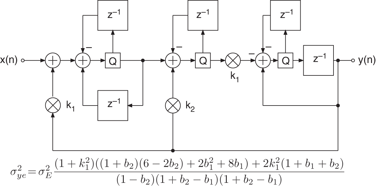
Figure 6.51 Kingsbury filter with noise shaping.
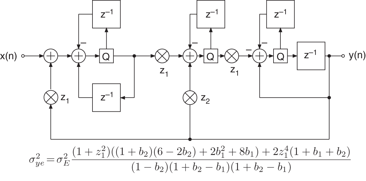
Figure 6.52 Zölzer filter with noise shaping.
The effect of noise shaping on SNR is shown in Figs. 6.53 and 6.54 . The almost ideal noise behavior of all filter structures for 16‐bit quantization and very small cutoff frequencies can be observed. The effect of this noise shaping for increasing cutoff frequencies is shown in Fig. 6.54 . The compensating effect of the two zeros at ![]() is reduced.
is reduced.
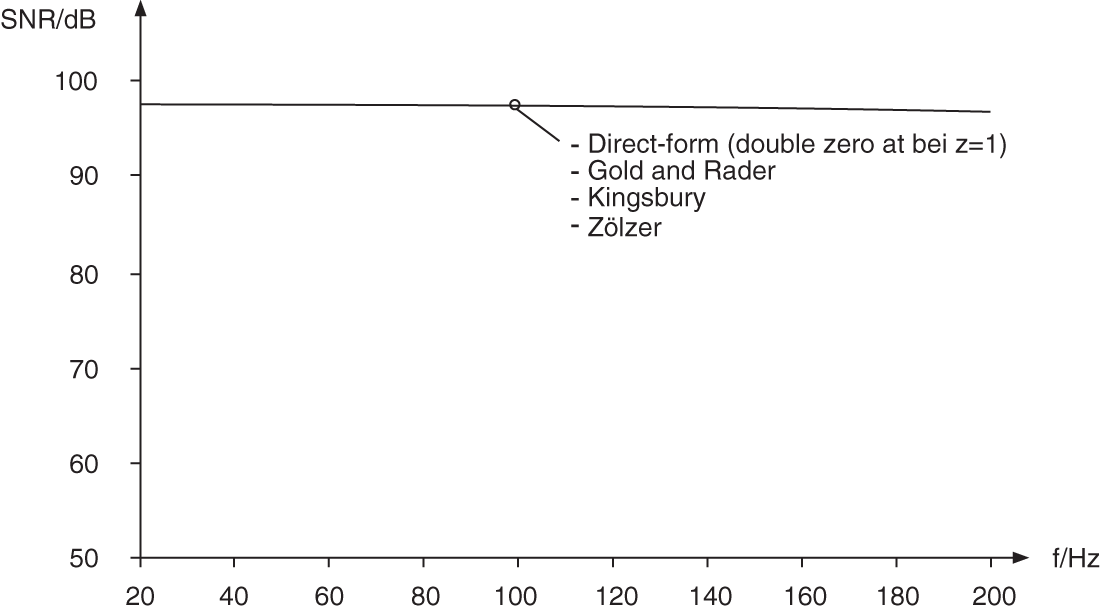
Figure 6.53 SNR – noise shaping (20–200 Hz).
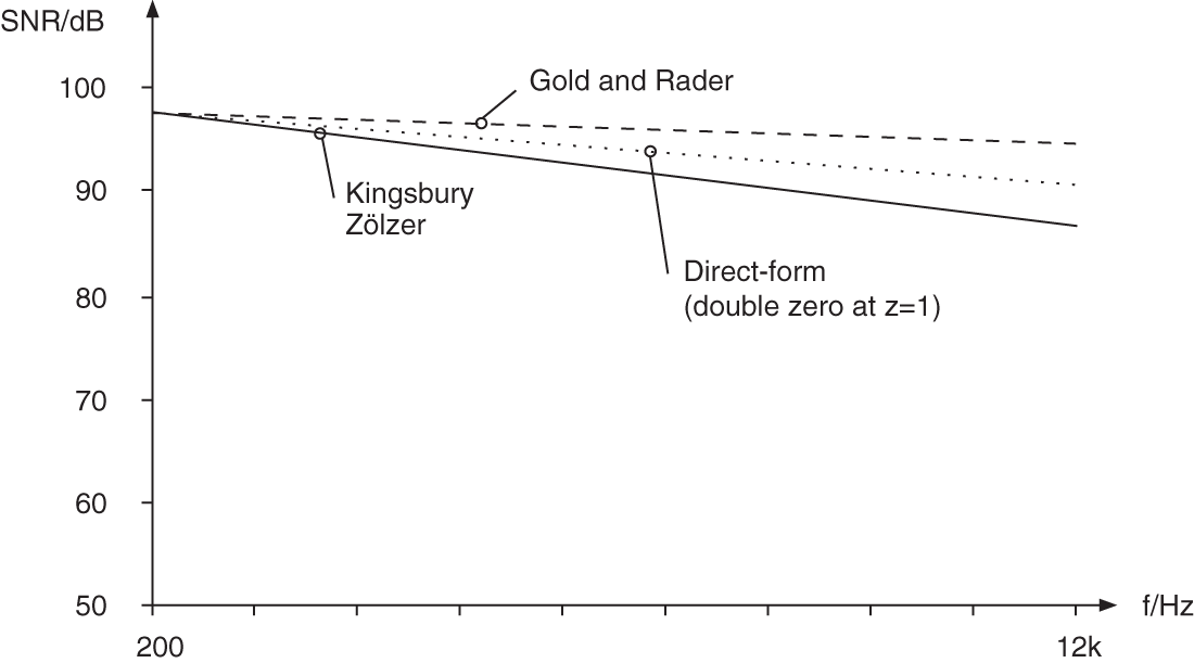
Figure 6.54 SNR – noise shaping (200 Hz–12 kHz).
Scaling
In a fixed‐point implementation of a digital filter, a transfer function from the input of the filter to a junction within the filter has to be determined, as well as the transfer function from the input to the output. By scaling the input signal, it has to be guaranteed that the signals remain within the number range at each junction and at the output.
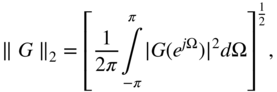
To calculate scaling coefficients, different criteria can be used. The ![]() norm is defined as
norm is defined as
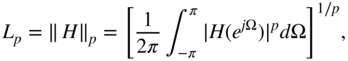
and an expression for the ![]() norm follows for
norm follows for ![]() :
:
The ![]() norm represents the maximum of the amplitude frequency response. In general, the modulus of the output is
norm represents the maximum of the amplitude frequency response. In general, the modulus of the output is
with
For the ![]() ,
, ![]() , and
, and ![]() norms, the explanations in Table 6.10 can be used.
norms, the explanations in Table 6.10 can be used.
Table 6.10 Commonly used scaling.
| p | q | |
|---|---|---|
| 1 | given max. value of input spectrum | |
| scaling w.r.t. the | ||
| 1 | given | |
| scaling w.r.t. the | ||
| 2 | 2 | given |
| scaling w.r.t. the |
With
the ![]() norm is given by
norm is given by
For a sinusoidal input signal of amplitude one, we get ![]() . For
. For ![]() to be valid, the scaling factor must be chosen to be
to be valid, the scaling factor must be chosen to be

The scaling of the input signal is carried out with the maximum of the amplitude frequency response with the goal that for ![]() ,
, ![]() . As a scaling coefficient for the input signal, the highest scaling factor
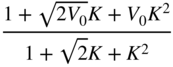
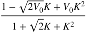
. As a scaling coefficient for the input signal, the highest scaling factor ![]() is chosen. For determining the maximum of the transfer function
is chosen. For determining the maximum of the transfer function
of a second‐order system
the maximum value can be calculated as
With ![]() , it follows that
, it follows that
The solution of Eq. (6.124) leads to ![]() , which must be real (
, which must be real (![]() ) for the maximum/minimum to occur at a real frequency. For a single solution (repeated roots) of the above quadratic equation, the discriminant must be
) for the maximum/minimum to occur at a real frequency. For a single solution (repeated roots) of the above quadratic equation, the discriminant must be ![]() (
(![]() ). It follows that
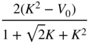
). It follows that
and
The solution of Eq. (6.126) gives two solutions for ![]() . The solution with the larger value is chosen. If the discriminant
. The solution with the larger value is chosen. If the discriminant ![]() is not greater than zero, the maximum lies at
is not greater than zero, the maximum lies at ![]() (
(![]() ) or
) or ![]() (
(![]() ), as given by
), as given by
or

Limit Cycles
Limit cycles are periodic processes in a filter which can be measured as sinusoidal signals. They arise owing to the quantization of state variables. The different types of limit cycle and the methods necessary to prevent them are briefly listed below:
- overflow limit cycles
 saturation curve
 scaling
 - limit cycles for vanishing input
 noise shaping
 dithering
 - limit cycles correlated with the input signal
 noise shaping
 dithering
6.3 Non‐recursive Audio Filters
For implementing linear phase audio filters, non‐recursive filters are used. The basis of an efficient implementation is the fast convolution
where the convolution in the time domain is performed by transforming the signal and the impulse response into the frequency domain, multiplication of the corresponding Fourier transforms, and inverse Fourier transform of the product into the time domain signal (see Fig. 6.55 ). The transform is carried out by a discrete Fourier transform of length ![]() , such that
, such that ![]() is valid and time‐domain aliasing is avoided.
is valid and time‐domain aliasing is avoided.

Figure 6.55 Fast convolution of signal  of length
  and impulse response
  of length
  delivers the convolution result
  of length
  .
.
First we will discuss the basics. We then introduce the convolution of long sequences followed by a filter design for linear phase filters.
6.3.1 Basics of Fast Convolution
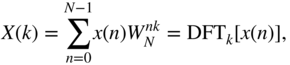
IDFT Implementation with DFT Algorithm. The discrete Fourier transformation (DFT) is described by
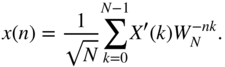
and the inverse discrete Fourier transformation (IDFT) by

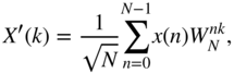
Without scaling factor ![]() , we write
, we write

so that the following symmetrical transformation algorithms hold:
The IDFT differs from the DFT only by its sign in the exponential term.
An alternative approach for calculating the IDFT with the help of a DFT is described as follows [Cad87, Duh88]. We will make use of the relationships
Conjugating Eq. (6.133) gives
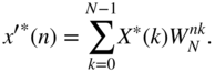
The multiplication of Eq. (6.138) by ![]() leads to
leads to

Conjugating and multiplying Eq. (6.139) by ![]() results in
results in
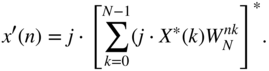
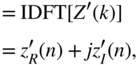
An interpretation of (Eqs. 6.137) and (6.140) suggests the following way of performing the IDFT with the DFT algorithm:
- exchange the real with the imaginary part of the spectral sequence

- transformation with DFT algorithm
- exchange the real with the imaginary part of the time sequence
For implementation on a digital signal processor, the use of DFT saves memory for IDFT.
Discrete Fourier Transformation of Two Real Sequences. In many applications, stereo signals that consist of a left and right channel are processed. With the help of the DFT, both channels can be transformed simultaneously into the frequency domain [Sor87, Ell82].
For a real sequence ![]() ,
,
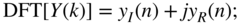
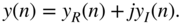
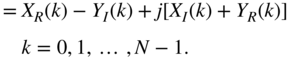
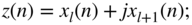
For a discrete Fourier transformation of two real sequences ![]() and
and ![]() , a complex sequence is first formed according to
, a complex sequence is first formed according to
The Fourier transformation gives
where
Because ![]() and
and ![]() are real sequences, it follows from Eq. (6.142) that
are real sequences, it follows from Eq. (6.142) that
Considering the real part of ![]() , adding (Eqs. 6.148) and (6.151) gives
, adding (Eqs. 6.148) and (6.151) gives
and subtraction of Eq. (6.151) from Eq. (6.148) results in
Considering the imaginary part of ![]() , adding (Eqs. 6.148) and (6.151) gives
, adding (Eqs. 6.148) and (6.151) gives
and subtraction of Eq. (6.151) from Eq. (6.148) results in
Hence the spectral functions are given by


and
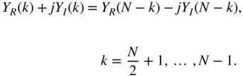
Fast Convolution if Spectral Functions are Known. The spectral functions ![]() ,
, ![]() , and
, and ![]() are known. With the help of Eq. (6.148), the spectral sequence can be formed by
are known. With the help of Eq. (6.148), the spectral sequence can be formed by
Filtering is done by multiplication in the frequency domain:

The inverse transformation gives
so that the filtered output sequence is given by
The filtering of a stereo signal can hence be done by transformation into the frequency domain, multiplication of the spectral functions, and inverse transformation of left and right channels.
6.3.2 Fast Convolution of Long Sequences
The fast convolution of two real input sequences ![]() and
and ![]() of length
of length ![]() with the impulse response
with the impulse response ![]() of length
of length ![]() leads to the output sequences
leads to the output sequences
of length ![]() . The implementation of a non‐recursive filter with fast convolution becomes more efficient than the direct implementation of an FIR filter for filter lengths
. The implementation of a non‐recursive filter with fast convolution becomes more efficient than the direct implementation of an FIR filter for filter lengths ![]() . Therefore, the following procedure will be performed:
. Therefore, the following procedure will be performed:
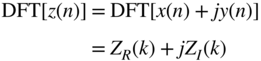
- formation of a complex sequence
(6.175)
- Fourier transformation of the impulse response
 that is padded with zeros to a length
  (6.176)
- Fourier transformation of the sequence
 that is padded with zeros to a length
 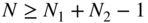 (6.177)
- formation of a complex output sequence
(6.178)
 (6.179)
 (6.180)
- formation of a real output sequence
(6.181)
 (6.182)
Figure 6.56 Fast convolution with partitioning of the input signal  into blocks of length
  .
.
For the convolution of an infinite‐length input sequence (see Fig. 6.56 ) with an impulse response ![]() , the input sequence is partitioned into sequences
, the input sequence is partitioned into sequences ![]() of length
of length ![]() :
:

The input sequence is given by superposition of finite‐length sequences according to

The convolution of the input sequence with the impulse response ![]() of length
of length ![]() gives
gives

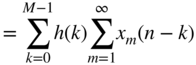

The term in brackets corresponds to the convolution of a finite‐length sequence ![]() of length
of length ![]() with the impulse response of length
with the impulse response of length ![]() . The output signal can be given as a superposition of convolution products of length
. The output signal can be given as a superposition of convolution products of length ![]() . With these partial convolution products,
. With these partial convolution products,

the output signal can be written as

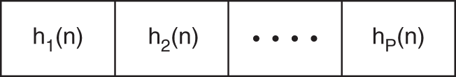
Figure 6.57 Partitioning of the impulse response  .
.
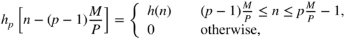
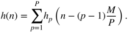
If the length ![]() of the impulse response is very long, it can be similarly partitioned into
of the impulse response is very long, it can be similarly partitioned into ![]() parts each of length
parts each of length ![]() (see Fig. 6.57 ). With
(see Fig. 6.57 ). With
it follows that
With ![]() and Eq. (6.189), the following partitioning can be done:
and Eq. (6.189), the following partitioning can be done:

This can be rewritten as
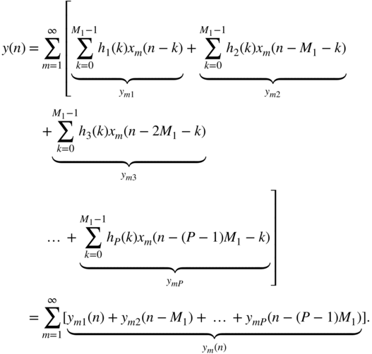
An example of partitioning the impulse response into ![]() parts is graphically shown in Fig. 6.58 . This leads to
parts is graphically shown in Fig. 6.58 . This leads to
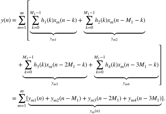

Figure 6.58 Scheme for a fast convolution with  .
.
The procedure of a fast convolution by partitioning the input sequence ![]() , as well as the impulse response
, as well as the impulse response ![]() , is given in the following for the example in Fig. 6.58 .
, is given in the following for the example in Fig. 6.58 .
- Decomposition of the impulse response
 of length
  :
(6.196)
:
(6.196) (6.197)
 (6.198)
 (6.199)
- Zero‐padding of partial impulse responses up to a length
 :
(6.200)
:
(6.200) (6.201)
 (6.202)
 (6.203)
- Calculating and storing
(6.204)

- Decomposition of the input sequence
 into partial sequences
  of length
  :
(6.205)
:
(6.205)
- Nesting partial sequences:
(6.206)

- Zero‐padding of complex sequence
 up to a length
  :
(6.207)
:
(6.207)
- Fourier transformation of the complex sequences
 :
(6.208)
:
(6.208)
- Multiplication in the frequency domain:
(6.209)
 (6.210)
 (6.211)
 (6.212)
 (6.213)
- Inverse transformation:
(6.214)
 (6.215)
 (6.216)
 (6.217)
- Determination of partial convolutions:
(6.218)
 (6.219)
 (6.220)
 (6.221)
 (6.222)
 (6.223)
 (6.224)
 (6.225)
- Overlap‐Add of partial sequences, increments
 and
and  , and back to step 5.
Based on the partitioning of the input signal and the impulse response and the following Fourier transform, the result of each single convolution is only available after a delay of one block of samples. Different methods to reduce computational complexity or overcome the block delay have been proposed [Soo90, Gar95, Ege96, Mül99, Mül01, Garc02]. These methods make use of a hybrid approach where the first part of the impulse response is used for time‐domain convolution and the other parts are used for fast convolution in the frequency domain. Figure 6.59 a,b demonstrates a simple derivation of the hybrid convolution scheme, which can be described by the decomposition of the transfer function according to

where the impulse response has length ![]() and
and ![]() is the number of smaller partitions of length
is the number of smaller partitions of length ![]() . Figure 6.59 c,d shows two different signal flow graphs for the decomposition given by Eq. (6.226) of the entire transfer function. Especially, Fig. 6.59 d highlights (with gray background) that in each branch
. Figure 6.59 c,d shows two different signal flow graphs for the decomposition given by Eq. (6.226) of the entire transfer function. Especially, Fig. 6.59 d highlights (with gray background) that in each branch ![]() , a delay of
, a delay of ![]() occurs and each filter
occurs and each filter ![]() has the same length and makes use of the same state variables. This means that they can be computed in parallel in the frequency domain with
has the same length and makes use of the same state variables. This means that they can be computed in parallel in the frequency domain with ![]() ‐FFTs/IFFTs and the outputs have to be delayed according to
‐FFTs/IFFTs and the outputs have to be delayed according to ![]() , as shown in Fig. 6.59 e. A further simplification shown in Fig. 6.59 f leads to one input
, as shown in Fig. 6.59 e. A further simplification shown in Fig. 6.59 f leads to one input ![]() ‐FFT and block delays
‐FFT and block delays ![]() for the frequency vectors. Then, parallel multiplications with
for the frequency vectors. Then, parallel multiplications with ![]() of length
of length ![]() and the summation of all intermediate products are performed before one output
and the summation of all intermediate products are performed before one output ![]() ‐IFFT for the overlap and add operation in the time domain is used. The first part of the impulse response, represented by
‐IFFT for the overlap and add operation in the time domain is used. The first part of the impulse response, represented by ![]() , is performed by direct convolution in the time domain. The frequency‐ and time‐domain parts are then overlapped and added. An alternative realization for fast convolution is based on the overlap and save operation.
, is performed by direct convolution in the time domain. The frequency‐ and time‐domain parts are then overlapped and added. An alternative realization for fast convolution is based on the overlap and save operation.

Figure 6.59 Hybrid fast convolution.
6.3.3 Filter Design by Frequency Sampling
Audio filter design for non‐recursive filter realizations by fast convolution can be carried out by the frequency sampling method. For linear phase systems,
where ![]() is a real valued amplitude response and
is a real valued amplitude response and ![]() is the length of the impulse response. The magnitude
is the length of the impulse response. The magnitude ![]() is calculated by sampling in the frequency domain at equidistant places
is calculated by sampling in the frequency domain at equidistant places
according to
Hence, a filter can be designed by fulfilling conditions in the frequency domain. The linear phase is determined as

Owing to the real transfer function ![]() for an even filter length, we have to fulfill
for an even filter length, we have to fulfill
This has to be taken into consideration when designing filters of even length ![]() . The impulse response
. The impulse response ![]() is obtained through an
is obtained through an ![]() ‐point IDFT of the spectral sequence
‐point IDFT of the spectral sequence ![]() . This impulse response is extended with zero‐padding to the length
. This impulse response is extended with zero‐padding to the length ![]() and then transformed by an
and then transformed by an ![]() ‐point DFT resulting in the spectral sequence
‐point DFT resulting in the spectral sequence ![]() of the filter.
of the filter.
6.4 Multi‐complementary Filter Bank
The sub‐band processing of audio signals is mainly used in source coding applications for efficient transmission and storing. The basis for the sub‐band decomposition is critically sampled filter banks [Vai93, Fli00]. These filter banks allow a perfect reconstruction of the input provided there is no processing within the sub‐bands. They consist of an analysis filter bank for decomposing the signal in critically sampled sub‐bands and a synthesis filter bank for reconstructing the broadband output. The aliasing in the sub‐bands is eliminated by the synthesis filter bank. Nonlinear methods are used for coding the sub‐band signals. The reconstruction error of the filter bank is negligible compared with the errors arising from the coding/decoding process. Using a critically sampled filter bank as a multiband equalizer, multiband dynamic range control, or multiband room simulation, the processing in the sub‐bands leads to aliasing at the output. To avoid aliasing, a multi‐complementary filter bank [Fli92, Zöl92, Fli00] is presented which enables an aliasing‐free processing in the sub‐bands and leads to a perfect reconstruction of the output. It allows a decomposition into octave frequency bands which are matched to the human ear.
6.4.1 Principles
Figure 6.61 shows an octave‐band filter bank with critical sampling. It performs a successive lowpass/highpass decomposition into half‐bands followed by downsampling by a factor of two. The decomposition leads to the sub‐bands ![]() to
to ![]() (see Fig. 6.62 ). The transition frequencies of this decomposition are given by
(see Fig. 6.62 ). The transition frequencies of this decomposition are given by
To avoid aliasing in sub‐bands, a modified octave‐band filter bank is considered, which is shown in Fig. 6.63 for a two‐band decomposition. The cutoff frequency of the modified filter bank is moved from ![]() to a lower frequency. This means that in downsampling the lowpass branch, no aliasing occurs in the transition band (e.g. cutoff frequency
to a lower frequency. This means that in downsampling the lowpass branch, no aliasing occurs in the transition band (e.g. cutoff frequency ![]() ). The broader highpass branch cannot be downsampled. A continuation of the described two‐band decomposition leads to the modified octave‐band filter bank shown in Fig. 6.64 . The frequency bands are depicted in Fig. 6.65 showing that besides the cutoff frequencies
). The broader highpass branch cannot be downsampled. A continuation of the described two‐band decomposition leads to the modified octave‐band filter bank shown in Fig. 6.64 . The frequency bands are depicted in Fig. 6.65 showing that besides the cutoff frequencies
the bandwidth of the sub‐bands is reduced by a factor of two. The highpass sub‐band ![]() is an exception.
is an exception.
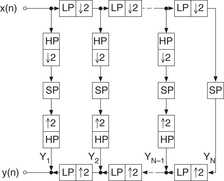
Figure 6.61 Octave‐band QMF bank (SP = signal processing, LP = lowpass, HP = highpass).
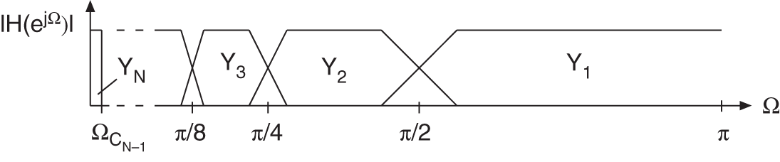
Figure 6.62 Octave‐frequency bands.
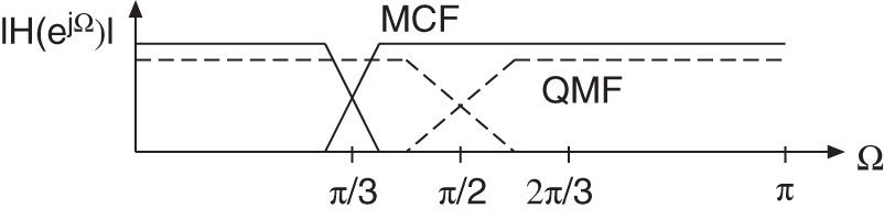
Figure 6.63 Two‐band decomposition.
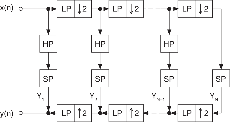
Figure 6.64 Modified octave‐band filter bank.

Figure 6.65 Modified octave decomposition.
The special lowpass/highpass decomposition is carried out by a two‐band complementary filter bank, as shown in Fig. 6.66 . The frequency responses of a decimation filter ![]() , interpolation filter
, interpolation filter ![]() , and kernel filter
, and kernel filter ![]() are shown in Fig. 6.67 .
are shown in Fig. 6.67 .
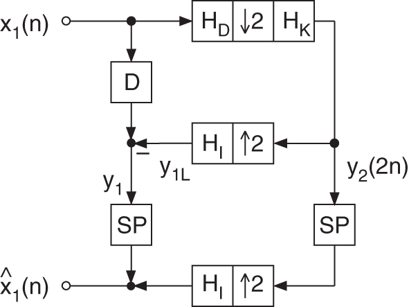
Figure 6.66 Two‐band complementary filter bank.
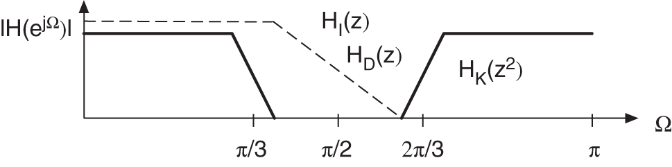
Figure 6.67 Design of  ,
,  , and
, and  .
.
The lowpass filtering of a signal ![]() is done with the help of a decimation filter
is done with the help of a decimation filter ![]() , the downsampler of factor two, and the kernel filter
, the downsampler of factor two, and the kernel filter ![]() , and leads to
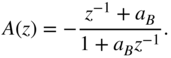
, and leads to ![]() . The Z‐transform of
. The Z‐transform of ![]() is given by
is given by
The interpolated lowpass signal ![]() is generated by upsampling by a factor of two and filtering with the interpolation filter
is generated by upsampling by a factor of two and filtering with the interpolation filter ![]() . The Z‐transform of
. The Z‐transform of ![]() is given by
is given by

The highpass signal ![]() is obtained by subtracting the interpolated lowpass signal
is obtained by subtracting the interpolated lowpass signal ![]() from the delayed input signal
from the delayed input signal ![]() . The Z‐transform of the highpass signal is given by
. The Z‐transform of the highpass signal is given by
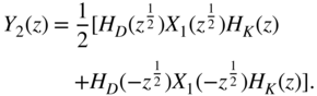
The lowpass and highpass signals are processed individually. The output signal ![]() is formed by adding the highpass signal to the upsampled and filtered lowpass signal. With (Eqs. 6.237) and (6.239), the Z‐transform of
is formed by adding the highpass signal to the upsampled and filtered lowpass signal. With (Eqs. 6.237) and (6.239), the Z‐transform of ![]() can be written as
can be written as
Equation (6.240) shows the perfect reconstruction of the input signal which is delayed by ![]() sampling units.
sampling units.
The extension to ![]() sub‐bands and implementing the kernel filter using complementary techniques [Ram88, Ram90] leads to the multi‐complementary filter bank, as shown in Fig. 6.68 . Delays are integrated in the highpass (
sub‐bands and implementing the kernel filter using complementary techniques [Ram88, Ram90] leads to the multi‐complementary filter bank, as shown in Fig. 6.68 . Delays are integrated in the highpass (![]() ) and bandpass sub‐bands (
) and bandpass sub‐bands (![]() to
to ![]() ) to compensate for the group delay. The filter structure consists of
) to compensate for the group delay. The filter structure consists of ![]() horizontal stages. The kernel filter is implemented as a complementary filter in
horizontal stages. The kernel filter is implemented as a complementary filter in ![]() vertical stages. The design of the latter shall be discussed later. The vertical delays in the extended kernel filters (
vertical stages. The design of the latter shall be discussed later. The vertical delays in the extended kernel filters (![]() to
to ![]() ) compensate group delays caused by forming the complementary component. At the end of each of these vertical stages is the kernel filter
) compensate group delays caused by forming the complementary component. At the end of each of these vertical stages is the kernel filter ![]() . With
. With
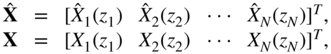
the signals ![]() can be written as a function of the signals
can be written as a function of the signals ![]() as
as
with
and with ![]() , the delays are given by
, the delays are given by
Perfect reconstruction of the input signal can be achieved if the horizontal delays ![]() are given by
are given by
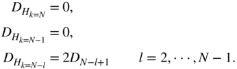

Figure 6.68 Multi‐complementary filter bank.
The implementation of the extended vertical kernel filters is done by calculating complementary components, as shown in Fig. 6.69 . After upsampling, interpolating with a highpass (Fig. 6.69 b) and forming the complementary component, the kernel filter ![]() with frequency response as in Fig. 6.69 a becomes lowpass with frequency response as illustrated in Fig. 6.69 c. The slope of the filter characteristic remains constant whereas the cutoff frequency is doubled. A subsequent upsampling with an interpolation highpass (Fig. 6.69 d) and complement filtering leads to the frequency response in Fig. 6.69 e. With the help of this technique, the kernel filter is implemented at a reduced sampling rate. The cutoff frequency is moved to a desired cutoff frequency by using decimation/interpolation stages with complement filtering.
with frequency response as in Fig. 6.69 a becomes lowpass with frequency response as illustrated in Fig. 6.69 c. The slope of the filter characteristic remains constant whereas the cutoff frequency is doubled. A subsequent upsampling with an interpolation highpass (Fig. 6.69 d) and complement filtering leads to the frequency response in Fig. 6.69 e. With the help of this technique, the kernel filter is implemented at a reduced sampling rate. The cutoff frequency is moved to a desired cutoff frequency by using decimation/interpolation stages with complement filtering.
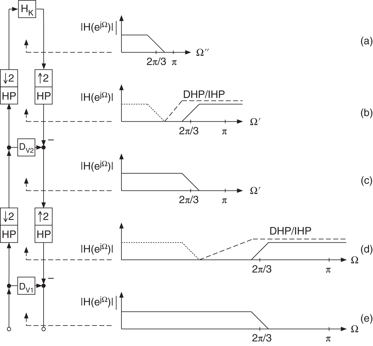
Figure 6.69 Multirate complementary filter.
Computational Complexity. For an ![]() ‐band multi‐complementary filter bank with
‐band multi‐complementary filter bank with ![]() decomposition filters, where each is implemented by a kernel filter with
decomposition filters, where each is implemented by a kernel filter with ![]() stages, the horizontal complexity is given by
stages, the horizontal complexity is given by
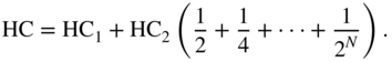
Here ![]() denotes the number of operations that are carried out at the input sampling rate. These operations occur in the horizontal stage
denotes the number of operations that are carried out at the input sampling rate. These operations occur in the horizontal stage ![]() (see Fig. 6.68 ). Furthermore,
(see Fig. 6.68 ). Furthermore, ![]() denotes the number of operations (horizontal stage
denotes the number of operations (horizontal stage ![]() ) that are performed at half of the sampling rate. The number of operations in the stages from
) that are performed at half of the sampling rate. The number of operations in the stages from ![]() to
to ![]() are approximately identical but are calculated at sampling rates that are successively halved.
are approximately identical but are calculated at sampling rates that are successively halved.
The complexities ![]() to
to ![]() of the vertical kernel filters
of the vertical kernel filters ![]() to
to ![]() are calculated as
are calculated as
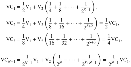
where ![]() depicts the complexity of the first stage
depicts the complexity of the first stage ![]() and
and ![]() is the complexity of the second stage
is the complexity of the second stage ![]() (see Fig. 6.68 ). It can be seen that the total vertical complexity is given by
(see Fig. 6.68 ). It can be seen that the total vertical complexity is given by
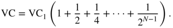
The upper bound of the total complexity results is the sum of horizontal and vertical complexities and can be written as
The total complexity ![]() is independent of the number of frequency bands
is independent of the number of frequency bands ![]() and vertical stages
and vertical stages ![]() . This means that for real‐time implementation with finite computation power, any desired number of sub‐bands with however narrow transition bands can be implemented.
. This means that for real‐time implementation with finite computation power, any desired number of sub‐bands with however narrow transition bands can be implemented.
6.4.2 Example: Eight‐band Multi‐complementary Filter Bank
To implement the frequency decomposition into the eight bands shown in Fig. 6.70 , the multirate filter structure of Fig. 6.71 is employed. The individual parts of the system provide means of downsampling (D=decimation), upsampling (I=interpolation), kernel filtering (K), signal processing (SP), delays (![]() =Delay 1,
=Delay 1, ![]() =Delay 2), and group delay compensation
=Delay 2), and group delay compensation ![]() in the
in the ![]() th band. The frequency decomposition is carried out successively from the highest to the lowest frequency band. In the two lowest frequency bands, a compensation for group delay is not required. The slope of the filter response can be adjusted with the kernel complementary filter structure shown in Fig. 6.72 which consists of one stage. The specifications of an 8‐band equalizer are listed in Table 6.11 . The stopband attenuation of the sub‐band filters is chosen to be 100 dB.
th band. The frequency decomposition is carried out successively from the highest to the lowest frequency band. In the two lowest frequency bands, a compensation for group delay is not required. The slope of the filter response can be adjusted with the kernel complementary filter structure shown in Fig. 6.72 which consists of one stage. The specifications of an 8‐band equalizer are listed in Table 6.11 . The stopband attenuation of the sub‐band filters is chosen to be 100 dB.
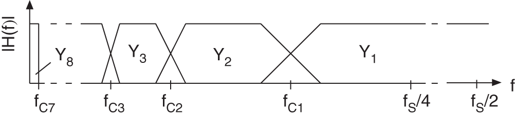
Figure 6.70 Modified octave decomposition of the frequency band.
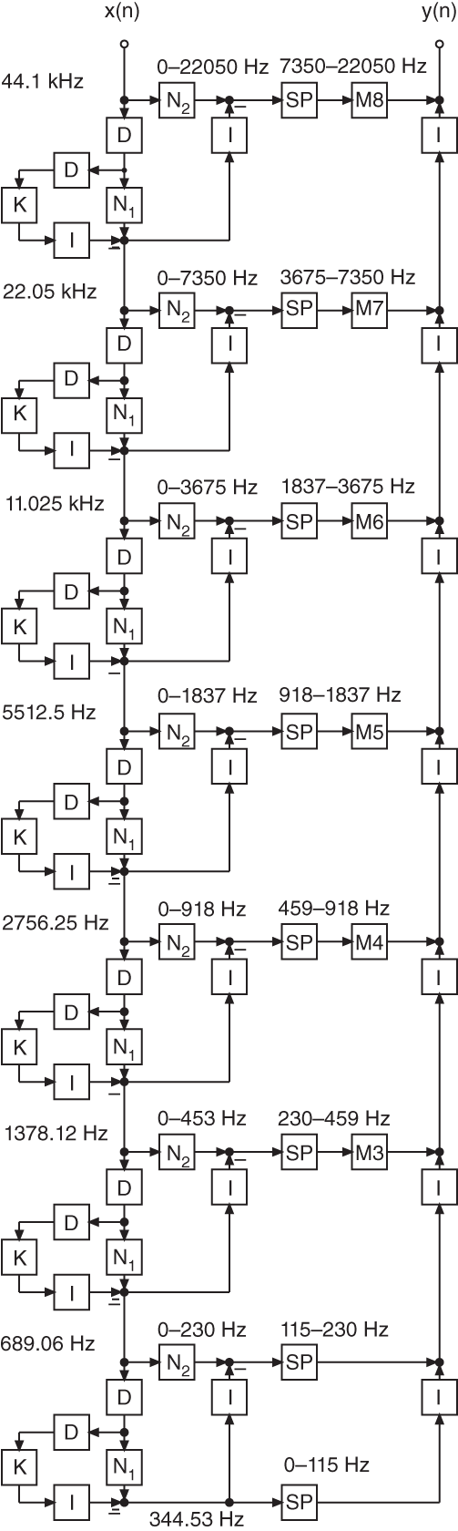
Figure 6.71 Linear phase 8‐band equalizer.
Table 6.11 Transition frequencies ![]() and transition bandwidths TB in an 8‐band equalizer.
and transition bandwidths TB in an 8‐band equalizer.
| 44.1 | 7350 | 3675 | 1837.5 | 918.75 | 459.375 | ||
| 1280 | 640 | 320 | 160 | 80 | 40 | 20 |
Filter Design
The design of different decimation and interpolation filters is mainly determined by the transition bandwidth and the stopband attenuation for the lower frequency band. As an example, a design is made for an 8‐band equalizer. The kernel complementary filter structure for both lower frequency bands is illustrated in Fig. 6.72 . The design specifications for the kernel lowpass, decimation, and interpolation filters are presented in Fig. 6.73 .
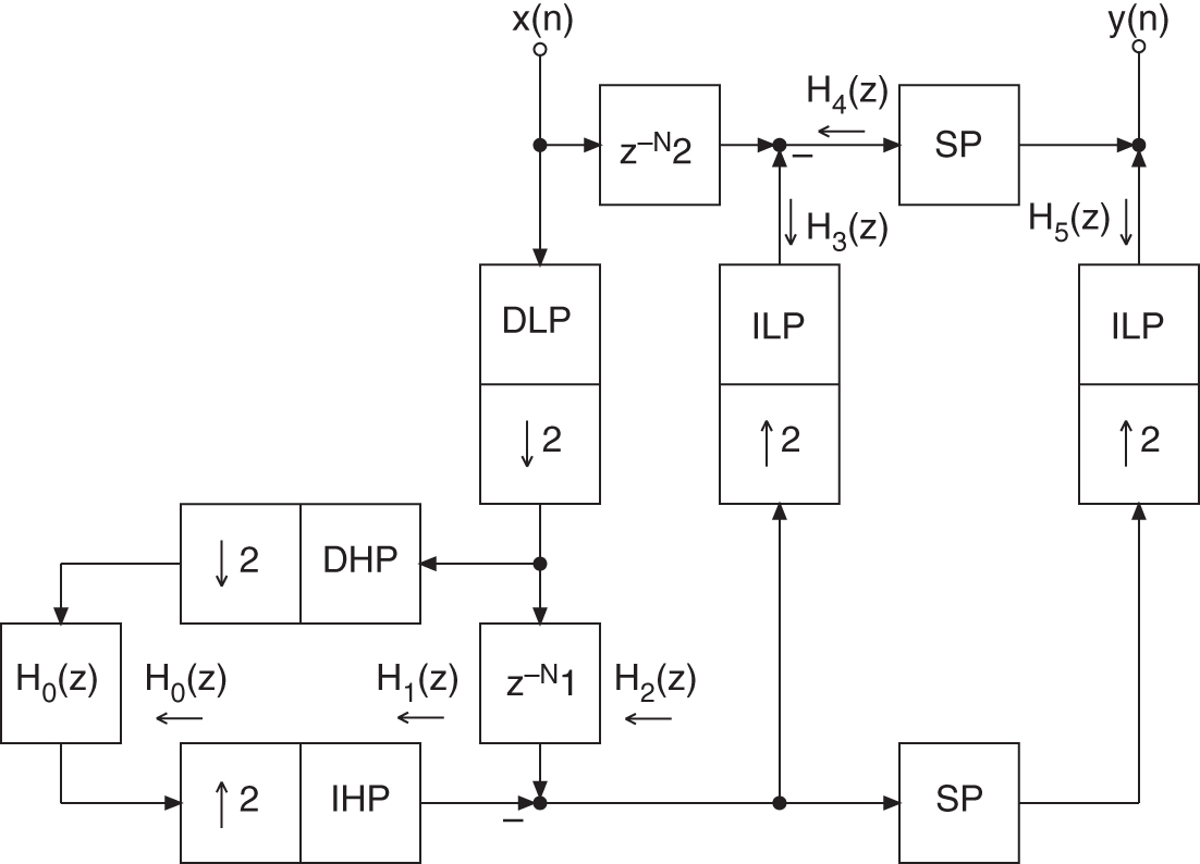
Figure 6.72 Kernel complementary filter structure.

Figure 6.73 Decimation and interpolation filters.
Kernel Filter Design. The transition bandwidth of the kernel filter is known if the transition bandwidth is given for the lower frequency band. This kernel filter must be designed for a sampling rate of ![]() . For a given transition bandwidth
. For a given transition bandwidth ![]() at a frequency
at a frequency ![]() , the normalized passband frequency is
, the normalized passband frequency is
and the normalized stopband frequency
With the help of these parameters, the filter can be designed. Making use of the Parks–McClellan program, the frequency response shown in Fig. 6.74 is obtained for a transition bandwidth of ![]() Hz. The necessary filter length for a stopband attenuation of 100 dB is 53 taps.
Hz. The necessary filter length for a stopband attenuation of 100 dB is 53 taps.
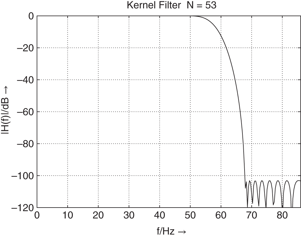
Figure 6.74 Kernel lowpass filter with a transition bandwidth of  Hz.
Hz.
Decimation and Interpolation Highpass Filter. These filters are designed for a sampling rate of ![]() and are half‐band filters, as illustrated in Fig. 6.73 . First a lowpass filter is designed followed by a highpass to lowpass transformation. For a given transition bandwidth
and are half‐band filters, as illustrated in Fig. 6.73 . First a lowpass filter is designed followed by a highpass to lowpass transformation. For a given transition bandwidth ![]() , the normalized passband frequency is
, the normalized passband frequency is

and the normalized stopband frequency is given by

With these parameters, the design of a half‐band filter is carried out. Figure 6.75 shows the frequency response. The necessary filter length for a stopband attenuation of 100 dB is 55 taps.
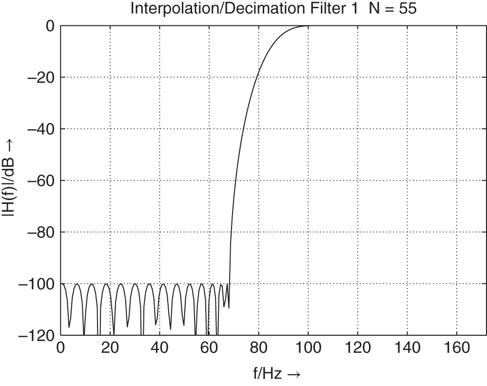
Figure 6.75 Decimation and interpolation highpass filter.
Decimation and Interpolation Lowpass Filter. These filters are designed for a sampling rate of ![]() and are also half‐band filters. For a given transition bandwidth
and are also half‐band filters. For a given transition bandwidth ![]() , the normalized passband frequency is
, the normalized passband frequency is

and the normalized stopband frequency is given by
With these parameters, the design of a half‐band filter is carried out. Figure 6.76 shows the frequency response. The necessary filter length for a stopband attenuation of 100 dB is 43 taps. These filter designs are used in every decomposition stage so that the transition frequencies and bandwidths are obtained as listed in Table 6.11 .
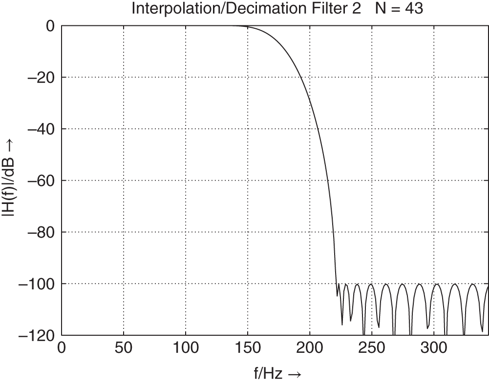
Figure 6.76 Decimation and interpolation lowpass filter.
Memory Requirements and Latency Time. The memory requirements depend directly on the transition bandwidth and the stopband attenuation. Here, the memory operations for the actual kernel, decimation, and interpolation filters have to be differentiated from the group delay compensations in the frequency bands. The compensating group delay ![]() for decimation and interpolation highpass filters of order
for decimation and interpolation highpass filters of order ![]() is calculated with the help of the kernel filter order
is calculated with the help of the kernel filter order ![]() according to
according to
The group delay compensation ![]() for the decimation and interpolation lowpass filters of order
for the decimation and interpolation lowpass filters of order ![]() is given by
is given by
The delays ![]() in the individual frequency bands are calculated recursively starting from the two lowest frequency bands:
in the individual frequency bands are calculated recursively starting from the two lowest frequency bands:

The memory requirements per decomposition stage are listed in Table 6.12 . The memory for the delays can be computed by ![]() . The latency time (delay) is given by
. The latency time (delay) is given by ![]() ms (
ms (![]() ms).
ms).
Table 6.12 Memory requirements.
| Kernel filter | |
| DHP/IHP | |
| DLP/ILP | |
6.5 Delay‐based Audio Effects
So far, we have discussed linear time‐invariant filtering using FIR and IIR systems with fixed coefficients over time. We will now introduce a time‐varying system which consists of a delay line where the length of that delay line is varied by a control signal ![]() , which is shown in the block diagram of Fig. 6.77 . Such a delay line modification [Dis99] performs a time‐varying delay of the input given by the relations:
, which is shown in the block diagram of Fig. 6.77 . Such a delay line modification [Dis99] performs a time‐varying delay of the input given by the relations:
The time‐varying delay of Eq. (6.256) leads to a phase modulation of the input ![]() , as shown by the Fourier transform given in Eq. (6.257). This delay line modulation can be achieved by linear interpolation between consecutive samples as shown by Eq. (6.258) performing fractional sample computation of the output
, as shown by the Fourier transform given in Eq. (6.257). This delay line modulation can be achieved by linear interpolation between consecutive samples as shown by Eq. (6.258) performing fractional sample computation of the output ![]() . Amplitude and phase modulation are used in the following four audio effects.
. Amplitude and phase modulation are used in the following four audio effects.

Figure 6.77 Phase modulation with delay line.
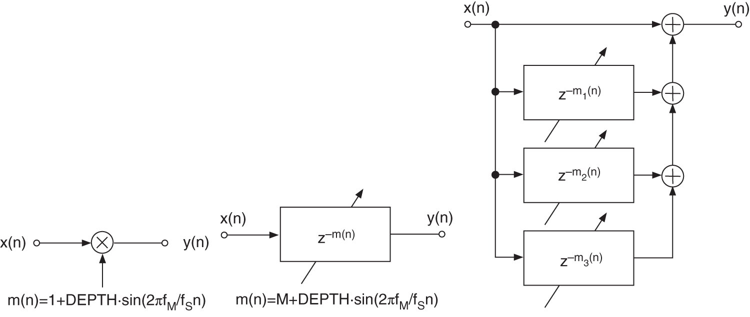
Figure 6.78 Tremolo, vibrato, and chorus effect.
- Tremolo is the rapid repetition of one note in music terminology or a rapid alternation between two or more notes (string instruments, mandolin, flute, piano, harpsichord, spinet, guitar). Tremolo is a rapid repetitive increase and decrease in volume. The effect is based on modifying the time‐domain envelope (amplitude) of a signal, as shown in the left part of Fig. 6.78 .
- Vibrato is the rapid and repetitive variation in pitch for the duration of a note (string instruments, guitar, singing voice, yodeling). As shown above, the effect is based on modifying the pitch of a signal by delay line modulation (phase modulation) shown in the middle part of Fig. 6.78 .
- Chorus simulates the result of an ensemble of musicians (singers, violins) playing together with slight pitch and amplitude differences. The chorus effect performs a loudness increase. These amplitude and pitch differences are simulated by amplitude modulation and delay line modulation (phase modulation) and all signals are summed together to form the output signal shown in the right part of Fig. 6.78 .
- A Flanger simulates a special filter effect which occurs if a slowly time‐varying single reflection is added to the direct signal (jet airplane effect). This effect can be achieved by playing two copies of a single signal from two tape machines while slowing down the replay speed of one tape machine by placing a finger to the flange of one tape reel.
6.6 JS Applet – Audio Filters
The applet shown in Fig. 6.79 demonstrates audio filters. It is designed for a first insight into the perceptual effect of filtering an audio signal. In addition to the different filter types and their acoustical effect, the applet offers a first insight into the logarithmic behavior of loudness and frequency resolution of our human acoustical perception.
The following filter functions can be selected on the lower right of the graphical user interface:
- Lowpass/highpass filter (LP/HP) with control parameter
- – cutoff frequency
 in Hertz (lower horizontal slider),
 - – all frequencies above (LP) or below (HP the cutoff frequency are attenuated according to the shown frequency response);
- – cutoff frequency
- Low‐/high‐frequency shelving filter (LFS/HFS) with control parameters
- – cutoff frequency
 in Hertz (lower horizontal slider),
 - – boost/cut in dB (left vertical slider with + for boost or ‐ for cut),
- – all frequencies below (LFS) or above (HFS) the cutoff frequency are boosted/cut according to the selected boost/cut;
- – cutoff frequency
- Peak filter with control parameters
- – center frequency
 in Hertz (lower horizontal slider),
 - – boost/cut in dB (left vertical slider with + for boost or ‐ for cut),
- –
 ‐factor
  (right vertical slider), which controls the bandwidth
  of the boost/cut around the adjusted center frequency
  . Lower
  ‐factor means wider bandwidth,
 - – the peak filter boosts/cuts the center frequency with a bandwidth adjusted by the
 ‐factor.
- – center frequency
The center window shows the frequency response (filter gain versus frequency) of the selected filter functions. You can choose between a linear and a logarithmic frequency axis.
You can choose between two predefined audio files from our web server (audio1.wav or audio2.wav) or your own local WAV file to be processed [Gui05].

Figure 6.79 JS applet – audio filters.
6.7 Exercises
1. Design of Recursive Audio Filters
- How can we design a low‐frequency shelving filter? Which parameters define the filter? Explain the control parameters.
- How can we derive a high‐frequency shelving filter? Which parameters define the filter?
- What is the difference between first‐ and second‐order shelving filters?
- How can we design a peak filter? Which parameters define the filter? What is the filter order? Describe the control parameters. Describe the
 ‐factor.
 - How do we derive the digital transfer function?
- Derive the digital transfer functions for the first‐order shelving filters.
2. Parametric Audio Filters
- What is the basic idea for parametric filters?
- What is the difference between the Regalia and the Zölzer filter structures? Count the number of multiplications and additions for both filter structures.
- Derive a signal flow graph for first‐ and second‐order parametric Zölzer filters with a direct‐form implementation of the allpass filters.
- Is there a complete decoupling of all control parameters for boost and cut? Which parameters are decoupled?
3. Shelving Filter: Direct Form
Derive a first‐order low‐shelving filter from a purely band‐limiting first‐order lowpass filter. Use bilinear transform and give the transfer function of the low‐shelving filter.
- State the filter coefficients and calculate the poles/zeros as functions of
 and
and  . Which gain factor do you have if
  ?
? - What is the difference between purely band‐limiting filters and shelving filter?
- How can you describe the boost and cut effect related to poles/zeros of the filter?
- How do we get a transfer function for the boost case from the cut case?
- How do we go from a low‐shelving filter to a high‐shelving filter?
4. Shelving Filter: Allpass Form
Implement a first‐order high‐shelving filter for the boost and cut case with the sampling rate ![]() kHz, the cutoff frequency
kHz, the cutoff frequency ![]() kHz, and the gain
kHz, and the gain ![]() dB.
dB.
- Define the allpass parameters and coefficients for the boost and cut case.
- Derive from the allpass decomposition the complete transfer function of the shelving filter.
- Using Matlab, give the magnitude frequency response for boost and cut. Show the result for the case where the boost and cut filters are in a series connection.
- If the input signal to the system is a unit impulse, give the spectrum of the input and output signal for the boost and cut case. What will you expect as result in this case when boost and cut are again cascaded?
5. Quantization of Filter Coefficients
For the quantization of the filter coefficients, different methods have been proposed: direct form, Gold and Rader, Kingsbury, and Zölzer.
- What is the motivation behind this?
- Plot a pole distribution using the quantized polar representation of a second‐order IIR filter

6. Signal Quantization Inside the Audio Filter
Now we combine coefficient and signal quantization.
- Design a digital highpass filter (second‐order IIR), with a cutoff frequency
 Hz.
Hz.
(Use the Butterworth, Chebyshev, or elliptic design methods implemented in Matlab.)
- Quantize the signal only when it leaves the accumulator (i.e. before it is saved in any state variable).
- Now quantize the coefficients (direct form) too.
- Extend your quantization to every arithmetic operation (i.e. after each addition/multiplication).
7. Quantization Effects in Recursive Audio Filters
- Why is the quantization of signals inside a recursive filter of special interest?
- Derive the noise transfer function of the second‐order direct‐form filter. Apply a first‐ and second‐order noise shaping to the quantizer inside the direct‐form structure and discuss the influence. What is the difference between second‐order noise shaping and double precision arithmetic?
- Write a Matlab implementation of a second‐order filter structure for quantization and noise shaping.
8. Fast Convolution
For an input sequence ![]() of length
of length ![]() and the impulse response
and the impulse response ![]() of length
of length ![]() , perform the discrete time convolution.
, perform the discrete time convolution.
- Give the discrete time convolution sum formula.
- Define with Matlab
 as the sum of two sinusoids and derive
  with Matlab function
  .
. - Realize the filter operation with Matlab using:
- the function
 ;
; - the sample by the sample convolution sum method;
- the FFT method;
- the FFT with the overlap and add method.
- the function
- Describe FIR filtering with the fast convolution technique. Which conditions have to be fulfilled for the input signal and the impulse response if convolution is performed by equivalent frequency‐domain processing?
- What happens if the input signal and impulse response are as long as the FFT transform length?
- How can we perform IFFT with the FFT algorithm?
- Explain the processing steps:
- for a segmentation of the input signal into blocks and fast convolution;
- for a stereo signal by the fast convolution technique;
- for the segmentation of the impulse response.
- What is the processing delay of the fast convolution technique?
- Write a Matlab program for fast convolution.
- How does quantization of the signal influence the roundoff noise behavior of an FIR filter?
9. FIR Filter Design by Frequency Sampling
- Why is frequency sampling an important design method for audio equalizers? How do we sample magnitude and phase response?
- What is a linear phase frequency response of a system? What is the effect on an input signal passing through such a system?
- Explain the derivation of the magnitude and phase response for a linear phase FIR filter.
- What is the condition for a real‐valued impulse response of even length
 ? What is the group delay?
 - Write a Matlab program for the design of an FIR filter and verify the example in the chapter.
- Now the desired frequency response is an ideal lowpass filter of length
 with cutoff frequency
  , derive the impulse response of this system. What will be the result for
  and
and  ?
?
10. Multi‐complementary Filter Bank
- What is octave‐spaced frequency splitting and how can we design a filter bank for that task?
- How can we perform aliasing‐free sub‐band processing? How can we achieve narrow transition bands for a filter bank? What is the computational complexity of an octave‐spaced filter bank?
References
- [Abu79] A.I. Abu‐El‐Haija, A.M. Peterson: An Approach to Eliminate Roundoff Errors in Digital Filters, IEEE Trans. ASSP, pp. 195–198, April 1979.
- [Ave71] E. Avenhaus: Zum Entwurf digitaler Filter mit minimaler Speicherwortlänge für Koeffizienten und Zustandsgrössen, Ausgewählte Arbeiten über Nachrichtensysteme, Nr. 13, herausgegeben von Prof. Dr.‐Ing. W. Schüssler, Erlangen 1971.
- [Bar82] C.W. Barnes: Error Feedback in Normal Realizations of Recursive Digital Filters, IEEE Trans. Circuits and Systems, pp. 72–75, Jan. 1982.
- [Bom85] B.W. Bomar: New Second‐Order State‐Space Structures for Realizing Low Roundoff Noise Digital Filters, IEEE Trans. ASSP, pp. 106–110, Feb. 1985.
- [Bri94] R. Bristow‐Johnson: The Equivalence of Various Methods of Computing Biquad Coefficients for Audio Parametric Equalizers, Proc. 97th AES Convention, Preprint No. 3906, November 1994.
- [Cad87] J.A. Cadzow: Foundations of Digital Signal Processing and Data Analysis, New York: Macmillan Publishing Company, 1987.
- [Cha78] T.L. Chang: A Low Roundoff Noise Digital Filter Structure, Proc. Int. Symp. on Circuits and Systems, pp. 1004–1008, May 1978.
- [Cla00] R.J. Clark, E.C. Ifeachor, G.M. Rogers, and P.W.J. Van Eetvelt: Techniques for Generating Digital Equalizer Coefficients, J. Audio Eng. Soc., Vol. 48, pp. 281–298, April 2000.
- [Cre03] L. Cremer, M. Möser: Technische Akustik, Springer‐Verlag, Berlin, 2003.
- [Dat97] J. Dattorro: Effect design ‐ Part 1: Reverberator and other Filters, J. Audio Eng. Soc., 45(19):660–684, September 1997.
- [Din95] Yinong Ding, D. Rossum: Filter Morphing of Parametric Equalizers and Shelving Filters for Audio Signal Processing, J. Audio Eng. Soc., Vol. 43, No.10, pp. 821–826, October 1995.
- [Dis99] S. Disch, U. Zölzer: Modulation and delay line based digital audio effects, In Proceedings of the COST G‐6 Conference on Digital Audio Effects (DAFX–99), Trondheim, Norway, December 9–11, 1999.
- [Duh88] P. Duhamel, B. Piron, J. Etcheto: On Computing the Inverse DFT, IEEE Trans. Acoust., Speech, Signal Processing, Vol. 36, No. 2, pp. 285–286, February 1988.
- [Ege96] G. P. M. Egelmeers and P. C. W. Sommen: A new method for efficient convolution in frequency domain by nonuniform partitioning for adaptive filtering, IEEE Trans. Signal Processing, Vol. 44, pp. 3123–3192, Dec. 1996.
- [Ell82] D.F. Elliott, K.R. Rao: Fast Transforms: Algorithms, Analyses, Applications, New York: Academic Press, 1982.
- [Fet72] A. Fettweis: On the Connection Between Multiplier Wordlength Limitation and Roundoff Noise in Digital Filters, IEEE Trans. Circuit Theory, pp. 486–491, Sept. 1972.
- [Fli92] N.J. Fliege, U. Zölzer: Multi‐Complementary Filter Bank: A New Concept with Aliasing‐Free Subband Signal Processing and Perfect Reconstruction, Proc. EUSIPCO‐92, Br″ussel, pp. 207–210, August 1992.
- [Fli93] N.J. Fliege, U. Zölzer: Multi‐Complementary Filter Bank, Proc. ICASSP‐93, Minneapolis, pp. 193–196, April 1993.
- [Fli00] N. Fliege: Multirate Digital Signal Processing, J. Wiley & Sons, Chichester, 2000.
- [Fon01] F. Fontana, M. Karjalainen: Magnitude‐complementary Filters for Dynamic Equalization, In Proc. of the DAFX‐01, Limerick, Ireland, pp. 97–101, Dec. 2001.
- [Fon03] F. Fontana, M. Karjalainen: A Digital Bandpass/Bandstop Complementary Equalization Filter with Independent Tuning Characteristics, IEEE Signal Processing Letters, vol. 10, n. 4, pp.119–122, Apr. 2003.
- [Gar95] W. G. Gardner: Efficient Convolution Without Input‐output Delay, J. Audio Eng. Soc., 43(3), pp. 127–136,1995.
- [Garc02] G. Garcia: Optimal Filter Partition for Efficient Convolution with Short Input/Output Delay, Proc. 113th AES Convention, Los Angeles, Preprint No. 5660, October 2002.
- [Gol67] B. Gold, C.M. Rader: Effects of Parameter Quantization on the Poles of a Digital Filter, Proc. IEEE, pp. 688–689, May 1967.
- [Gui05] M. Guillemard, C. Ruwwe, U. Zölzer: J‐DAFx ‐ Digital Audio Effects in Java, Proc. 8th Int. Conference on Digital Audio Effects (DAFx‐05), Madrid, Spain, pp.161–166, 2005.
- [Har93] F.J. Harris, E. Brooking: A Versatile Parametric Filter Using an Imbedded All‐Pass Sub‐Filter to Independently Adjust Bandwidth, Center Frequency and Boost or Cut, Proc. 95th AES Convention, San Francisco, Preprint No. 3757, 1993.
- [Här98] A. Härmä: Implementation of Recursive Filters Having Delay Free Loops, Proc. IEEE Int. Conf. Acoustics, Speech, and Signal Processing (ICASSP'98), Vol. 3, pp. 1261–1264, Seattle, Washington, 1998.
- [Hol06a] M. Holters, U. Zölzer: Parametric Recursive Higher‐Order Shelving Filters, Jahrestagung Akustik DAGA, 20.‐23. März 2006, Braunschweig, 2006.
- [Hol06b] M. Holters, U. Zölzer: Parametric recursive higher‐order shelving filters, Proc. 120th Conv. Audio Eng. Soc., Preprint No. 6722, Paris, 2006.
- [Hol06c] M. Holters, U. Zölzer: Parametric Higher‐Order Shelving Filters, Proc. EUSIPCO‐06, Florence, 2006.
- [Hol06d] M. Holters, U. Zölzer: Graphic Equalizer Design Using Higher‐Order Recursive Filters, Proc. of the 9th Int. Conference on Digital Audio Effects (DAFx‐06), Montreal, Canada, September 18‐20, pp. 37–40, 2006.
- [Jur64] E.I. Jury: Theory and Application of the z‐Transform Method, Wiley, 1964.
- [Kei04] F. Keiler, U. Zölzer, Parametric Second‐ and Fourth‐Order Shelving Filters for Audio Applications, Proc. of IEEE 6th International Workshop on Multimedia Signal Processing, Siena, Italy, September 29 ‐ October 1, 2004.
- [Kin72] N.G. Kingsbury: Second‐Order Recursive Digital Filter Element for Poles Near the Unit Circle and the Real z‐Axis, Electronic Letters, pp. 155–156, March 1972.
- [Moo83] J.A. Moorer: The Manifold Joys of Conformal Mapping, J. Audio Eng. Soc., Vol. 31, pp. 826–841, 1983.
- [Mou90] J.N. Mourjopoulos, E.D. Kyriakis‐Bitzaros, C.E. Goutis: Theory and Real‐time Implementation of Time‐varying Digital Audio Filters, J. Audio Eng. Soc., Vol. 38, pp. 523–536, July/August 1990.
- [Mul76] C.T. Mullis, R.A. Roberts: Synthesis of Minimum Roundoff Noise Fixed Point Digital Filters, IEEE Trans. Circuits and Systems, pp. 551–562, Sept. 1976.
- [Mül99] C. Müller‐Tomfelde: Low Latency Convolution for Real‐time Application, In Proceedings of the AES 16th International Conference: Spatial Sound Reproduction, Rovaniemi, Finland, April 10‐12, pp. 454–460, 1999.
- [Mül01] C. Müller‐Tomfelde: Time‐Varying Filter in Non‐Uniform Block Convolution, In Proceedings of the COST G‐6 Conference on Digital Audio Effects (DAFX‐01), Limerick, Ireland, December 6–8, 2001.
- [Orf96a] S.J. Orfanidis: Introduction to Signal Processing. Prentice‐Hall, 1996.
- [Orf96b] S.J. Orfanidis: Digital Parametric Equalizer Design with Prescribed Nyquist‐Frequency Gain, Proc. 101st Convention Audio Engineering Society, Preprint No. 4361, November 1996.
- [Orf05] S.J. Orfanidis: High‐order digital parametric equalizer design, J. Audio Eng. Soc., Vol. 53, No. 11, pp. 1026–1046, 2005.
- [Rab88] R. Rabenstein: Minimization of Transient Signals in Recursive Time‐varying Digital Filters, Circuits, Systems, and Signal Processing, Vol. 7, No. 3, pp. 345–359, 1988.
- [Ram88] T.A. Ramstad, T. Saramäki: Efficient Multirate Realization for Narrow Transition‐Band FIR Filters, Proc. IEEE Int. Symp. on Circuits and Syst. (Espoo, Finland), pp. 2019–2022, June 1988.
- [Ram90] T.A. Ramstad, T. Saramäki: Multistage, Multirate FIR Filter Structures for Narrow Transition‐Band Filters, Proc. IEEE Int. Symp. on Circuits and Syst. (New Orleans, USA), pp. 2017–2021, May 1990.
- [Reg87] P.A. Regalia, S.K. Mitra: Tunable Digital Frequency Response Equalization Filters, IEEE Transactions on Acoustics, Speech, and Signal Processing, Vol. 35, No. 1, pp. 118–120, January 1987.
- [Sha92] D.J. Shpak: Analytical Design of Biquadradic Filter Sections for Parametric Filters, J. Audio Eng. Soc., Vol. 40, pp. 876–885, November 1992.
- [Soo90] J.S. Soo, K.K. Pang: Multidelay Block Frequency Domain Adaptive Filter, IIEEE Transactions on Acoustics, Speech, and Signal Processing, Vol. 38, No. 2, pp. 373–376, Feb. 1990.
- [Sor87] H.V. Sorensen, D.J. Jones, M.T. Heideman, C.S. Burrus: Real‐Valued Fast Fourier Transform Algorithms, IEEE Trans. Acoust., Speech, Signal Processing, Vol. 35, No. 6, pp. 849–863, June 1987.
- [Sri77] A.B. Sripad, D.L. Snyder: A Necessary and Sufficient Condition for Quantization Errors to be Uniform and White, IEEE Trans. ASSP, Vol. 25, pp. 442–448, Oct. 1977.
- [Tra77]Tran‐Thong, B. Liu: Error Spectrum Shaping in Narrow Band Recursive Filters, IEEE Trans. ASSP, pp. 200–203, April 1977.
- [Vai93] P.P. Vaidyanathan: Multirate Systems and Filter Banks, Prentice‐Hall, Englewood Cliffs, 1993.
- [Väl98] V. Välimäki, T.I. Laakso: Suppression of Transients in Time‐varying Recursive Filters for Audio Signals, Proc. IEEE Int. Conf. Acoustics, Speech, and Signal Processing (ICASSP'98), Vol. 6, pp. 3569–3572, Seattle, Washington, 1998.
- [Väl16] V. Välimäki and J.D. Reiss: All about audio equalization: Solutions and frontiers. Applied Sciences, 6(5), 2016.
- [Whi86] S.A. White: Design of a Digital Biquadratic Peaking or Notch Filter for Digital Audio Equalization, J. Audio Eng. Soc., Vol. 34, pp. 479–483, 1986.
- [Zöl89] U. Zölzer: Entwurf digitaler Filter für die Anwendung im Tonstudiobereich, Wissenschaftliche Beiträge zur Nachrichtentechnik und Signalverarbeitung, TU Hamburg‐Harburg, Juni 1989.
- [Zöl90] U. Zölzer: A Low Roundoff Noise Digital Audio Filter, Proc. EUSIPCO‐90, Barcelona, pp. 529–532, 1990.
- [Zöl92] U. Zölzer, N. Fliege: Logarithmic Spaced Analysis Filter Bank for Multiple Loudspeaker Channels, Proc. 93rd AES Convention, Preprint No. 3453, San Francisco 1992.
- [Zöl93] U. Zölzer, B. Redmer, J. Bucholtz: Strategies for Switching Digital Audio Filters, Proc. 95th AES Convention, New York, Preprint No. 3714, October 1993.
- [Zöl94] U. Zölzer: Roundoff Error Analysis of Digital Filters, J. Audio Eng. Soc., Vol. 42, No. 4, pp. 232–244, April 1994.
- [Zöl95] U. Zölzer, T. Boltze: Parametric Digital Filter Structures, Proc. 99th AES Convention, New York, Preprint No. 4099, October 1995.