
Chapter 1
Introduction
U. Zölzer
In this first chapter, we will introduce the basics of signals and systems, and describe the transmission of signals through these systems [Opp14]. These fundamental concepts and the describing algorithms lay the foundation for digital audio signal processing. We will start with analog signals and analog systems, then we will sample the analog signals and perform digital signal processing, and finally reconstruct an analog output signal from the digital output signal. Figure 1.1 shows a typical audio application of capturing a vocalist and transmission to a loudspeaker via an amplifier for reproduction in another room for a listener or listening audience. The microphone delivers an electrical input signal ![]() and the output signal
and the output signal ![]() is the signal that will be received by the listener's ear. Both signals are continuous‐time input and output signals. The entire chain of operations from microphone, amplifier, loudspeaker, and sound transmission through the listening room to the listener can be modeled by a system with a continuous‐time impulse response
is the signal that will be received by the listener's ear. Both signals are continuous‐time input and output signals. The entire chain of operations from microphone, amplifier, loudspeaker, and sound transmission through the listening room to the listener can be modeled by a system with a continuous‐time impulse response ![]() . Such an impulse response can be acquired by an impulse response measurement approach. The entire continuous‐time approach description can also be represented by a discrete‐time approach through sampling the microphone signal
. Such an impulse response can be acquired by an impulse response measurement approach. The entire continuous‐time approach description can also be represented by a discrete‐time approach through sampling the microphone signal ![]() , using the discrete‐time impulse response
, using the discrete‐time impulse response ![]() , and then delivering the output signal
, and then delivering the output signal ![]() . Both continuous‐time and discrete‐time signal‐processing techniques [Opp10, Opp14] will be introduced in the following sections.
. Both continuous‐time and discrete‐time signal‐processing techniques [Opp10, Opp14] will be introduced in the following sections.
1.1 Continuous‐time Signals and Convolution
Continuous‐time signals ![]() , as shown in Fig. 1.2, can be used as test signals to analyze the behavior of the response of a physical system to an excitation signal. We need a few simple test signals that will allow for the derivation of all important relations to obtain the input/output description of an input signal transformed to an output signal (handclap
, as shown in Fig. 1.2, can be used as test signals to analyze the behavior of the response of a physical system to an excitation signal. We need a few simple test signals that will allow for the derivation of all important relations to obtain the input/output description of an input signal transformed to an output signal (handclap ![]() acoustical transmission through room
acoustical transmission through room ![]() received by human ear). The rectangular (rect) function is defined by
received by human ear). The rectangular (rect) function is defined by
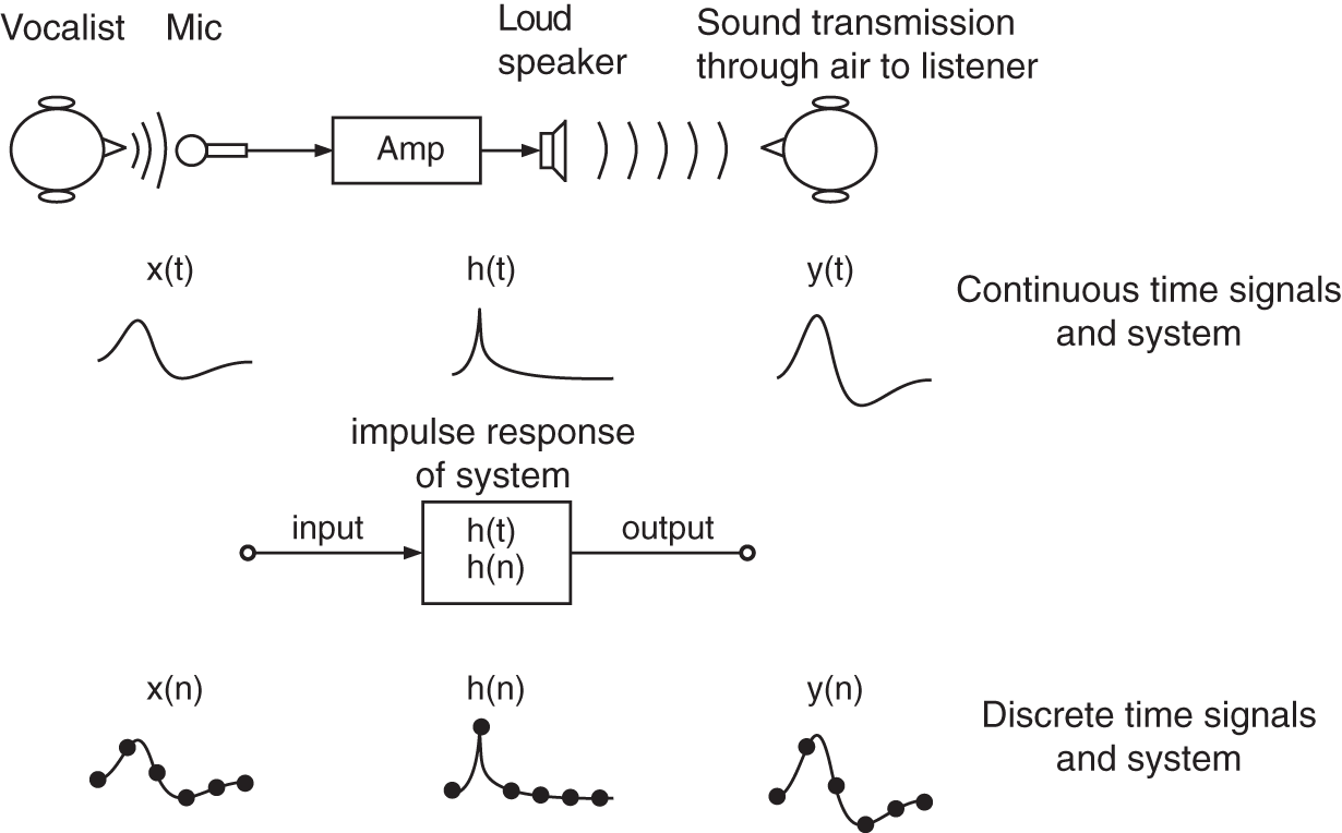
Figure 1.1 Audio capturing and reproduction for a listener, and representations of the operations by a signal and system model with input and output signals and by a system represented by an impulse response.

Figure 1.2 Continuous‐time signals  ,
,  ,
,  ,
,  ,
,  , and
, and  .
.

The Dirac impulse ![]() is defined by
is defined by

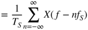
The step function is defined by

A general signal ![]() can be written using the sampling property of the Dirac impulse as
can be written using the sampling property of the Dirac impulse as

Continuous‐time systems transform the input ![]() to the output
to the output ![]() . A time‐domain description can be given by the following signal flow graph:
. A time‐domain description can be given by the following signal flow graph: ![]() . The system parameter inside the box is called the impulse response
. The system parameter inside the box is called the impulse response ![]() of the system. It describes the output of the system
of the system. It describes the output of the system ![]() when the input is the Dirac
when the input is the Dirac ![]() . Using Eq. (1.4), we can easily derive that the input/output relation of a system with impulse response
. Using Eq. (1.4), we can easily derive that the input/output relation of a system with impulse response ![]() is given by the integral (sliding the folded impulse response
is given by the integral (sliding the folded impulse response ![]() along the input and performing weighting and integration)
along the input and performing weighting and integration)

which is called continuous‐time convolution. The convolution integral describes a filter operation and is written as ![]() . Causality of a system implies
. Causality of a system implies ![]() for
for ![]() and stability of a system is achieved if the integral of impulse response
and stability of a system is achieved if the integral of impulse response ![]() . A simple example for continuous‐time convolution is demonstrated in Fig. 1.3.
. A simple example for continuous‐time convolution is demonstrated in Fig. 1.3.
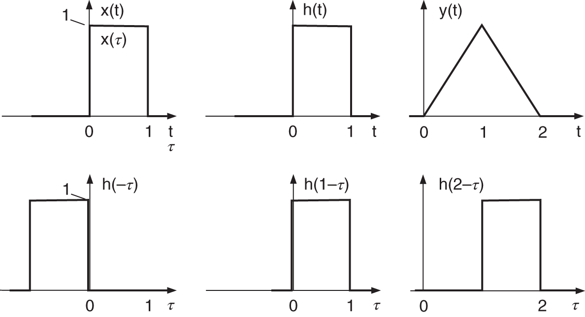
Figure 1.3 Continuous‐time convolution  showing the folded version of the impulse response
  and shifted versions
  for
for  .
.
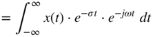
Using the complex exponential ![]() as input with
as input with ![]() , the output is given by the convolution integral as
, the output is given by the convolution integral as
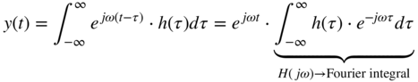
This shows that for a exponential input ![]() , the output
, the output ![]() is again an exponential signal where the input signal is weighted by the complex number
is again an exponential signal where the input signal is weighted by the complex number ![]() , which is the Fourier transform (integral) of the impulse response
, which is the Fourier transform (integral) of the impulse response ![]() , and is also called the frequency response of a continuous‐time system given by
, and is also called the frequency response of a continuous‐time system given by

From ![]() , we can compute the magnitude response
, we can compute the magnitude response
and the phase response

of a continuous‐time system. For a given signal ![]() , we can give its continuous‐time Fourier transform as
, we can give its continuous‐time Fourier transform as

The Fourier integral describes a spectral transform from time domain ![]() to frequency domain
to frequency domain ![]() , which is called the Fourier spectrum or Fourier transform of
, which is called the Fourier spectrum or Fourier transform of ![]() . The inverse continuous‐time Fourier transform is given by
. The inverse continuous‐time Fourier transform is given by
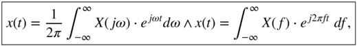
which takes the Fourier spectrum ![]() and reconstructs the input
and reconstructs the input ![]() . In the following, useful Fourier transform pairs are listed in Eqs. (1.13)–(1.23). An important relation between the time domain
. In the following, useful Fourier transform pairs are listed in Eqs. (1.13)–(1.23). An important relation between the time domain ![]() , using
, using ![]() and
and ![]() giving
giving ![]() , and frequency domain
, and frequency domain ![]() , using
, using ![]() and
and ![]() giving
giving ![]() , shows that convolution in the time domain can be described by multiplication in the frequency domain.
, shows that convolution in the time domain can be described by multiplication in the frequency domain.
Fourier Transform Pairs1

Fourier Transforms of Even and Causal Signals
Figure 1.4 shows the Fourier transforms of even and causal rect signals and Fig. 1.5 shows two even sinc signals and their Fourier transforms. The ripple in the passband is based on the truncated length of the sinc signal.

Figure 1.4 Fourier transforms of an even and a causal rect signal. The small imaginary part of the lower left plot arises from a small asymmetry of the rect signal in the upper left plot.

Figure 1.5 Fourier transforms of two even sinc signals.
1.2 Continuous‐time Fourier Transform and Laplace Transform
The extension of the continuous‐time Fourier transform to the Laplace transform allows for the transform of signals and impulse responses where the Fourier transform does not converge but the Laplace transform converges for a given convergence region. This extension of the continuous‐time Fourier transform

is achieved by introducing a real part to the imaginary part according to a new complex variable ![]() , which then gives
, which then gives

and thus the Laplace transform
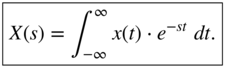
The Laplace transform of signals often leads to a rational function ![]() with a numerator polynomial
with a numerator polynomial ![]() and a denominator polynomial
and a denominator polynomial ![]() in the variable
in the variable ![]() . The zeros of the numerator
. The zeros of the numerator ![]() are called the zeros of
are called the zeros of ![]() and the zeros of
and the zeros of ![]() are called the poles of
are called the poles of ![]() . The rational function
. The rational function ![]() can be in given in polynomial, pole/zero, and partial expansion forms.
can be in given in polynomial, pole/zero, and partial expansion forms.
1.3 Sampling and Reconstruction
For digital signal processing, the sampling of ![]() with a sampling rate
with a sampling rate ![]() and a sampling interval
and a sampling interval ![]() is performed, which leads to a sequence of numbers
is performed, which leads to a sequence of numbers ![]() with time index
with time index ![]() . According to the sampling theorem, the input signal
. According to the sampling theorem, the input signal ![]() must be band limited to
must be band limited to ![]() . The sampling and the reconstruction of
. The sampling and the reconstruction of ![]() from the number sequence
from the number sequence ![]() is achieved by the following sequence of operations:
is achieved by the following sequence of operations: ![]() . Both operations are performed by an analog‐to‐digital converter (ADC) and a digital‐to‐analog converter (DAC). The converters can be considered as mixed continuous‐time and discrete‐time systems.
. Both operations are performed by an analog‐to‐digital converter (ADC) and a digital‐to‐analog converter (DAC). The converters can be considered as mixed continuous‐time and discrete‐time systems.
Sampling and quantization (analog‐to‐digital conversion) can be described by

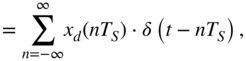
where the input ![]() is sampled by multiplying it with a series of Dirac impulses
is sampled by multiplying it with a series of Dirac impulses ![]() giving the ideal sampled
giving the ideal sampled ![]() and then quantization of the samples
and then quantization of the samples ![]() to the sequence of numbers
to the sequence of numbers ![]() with a finite number representation. Figure 1.6 shows in the left column the time‐domain signals involved.
with a finite number representation. Figure 1.6 shows in the left column the time‐domain signals involved.

Figure 1.6 Sampling and reconstruction – Time‐domain signals (left column) and corresponding Fourier spectra (right column).
Reconstruction (digital‐to‐analog conversion) of the continuous‐time ![]() from the sampled sequence
from the sampled sequence ![]() can be written as a convolution operation given by
can be written as a convolution operation given by
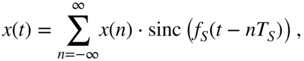
which is shown in the bottom left plot of Fig. 1.6. The Fourier transforms of the individual signals for sampling are given by
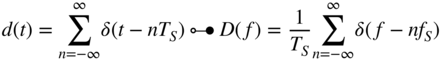
and are shown in Fig. 1.6 (right column). Sampling leads to the periodic extension of the baseband spectrum at multiples of the sampling rate ![]() and the scaling by
and the scaling by ![]() . The reconstruction of
. The reconstruction of

is achieved by convolution with a system impulse response ![]() , which acts an ideal lowpass filter with cutoff frequency
, which acts an ideal lowpass filter with cutoff frequency ![]() and passband gain of
and passband gain of ![]() to compensate for the scaling of the sampling operation, as shown in the bottom plots of Fig. 1.6.
to compensate for the scaling of the sampling operation, as shown in the bottom plots of Fig. 1.6.
1.4 Discrete‐time Signals and Convolution
With the discrete‐time input signal ![]() , we can describe an input/output relation in the discrete‐time domain, in signal flow graph form, as
, we can describe an input/output relation in the discrete‐time domain, in signal flow graph form, as ![]() , where the input is transformed into an output signal
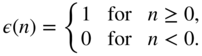
, where the input is transformed into an output signal ![]() . Again we are using discrete‐time test signals represented in Fig. 1.7, such as the unit pulse
. Again we are using discrete‐time test signals represented in Fig. 1.7, such as the unit pulse

and the step sequence
The lower row in Fig. 1.7 shows further discrete‐time signals which can be formulated using delayed unit pulses ![]() according to
according to

Figure 1.7 Discrete‐time signals  ,
,  ,
,  ,
,  ,
,  , and
, and  .
.

Figure 1.8 Discrete‐time convolution  showing the folded version of the impulse response
  and shifted versions
  for
for  .
.
and explicitly as, for example, ![]() . The discrete‐time system described by
. The discrete‐time system described by ![]() leads to the definition of the impulse response
leads to the definition of the impulse response ![]() of the discrete‐time system when the unit pulse
of the discrete‐time system when the unit pulse ![]() is used as an input signal
is used as an input signal ![]() . Using Eq. (1.40), we can derive the discrete‐time convolution as
. Using Eq. (1.40), we can derive the discrete‐time convolution as
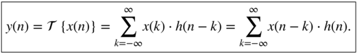
The convolution sum describes a digital filter operation and is written as ![]() . The discrete‐time convolution is illustrated in Fig. 1.8. Causality of a discrete‐time system implies
. The discrete‐time convolution is illustrated in Fig. 1.8. Causality of a discrete‐time system implies ![]() for
for ![]() and stability of a discrete‐time system is achieved if
and stability of a discrete‐time system is achieved if ![]() .
.
Using the complex exponential ![]() as input with
as input with ![]() , the output is given by the convolution sum as
, the output is given by the convolution sum as

This shows that for an exponential input ![]() , the output
, the output ![]() is again an exponential signal where the input signal is weighted by the complex number
is again an exponential signal where the input signal is weighted by the complex number ![]() , which is the discrete‐time Fourier transform of the impulse response
, which is the discrete‐time Fourier transform of the impulse response ![]() , and is also called the frequency response
, and is also called the frequency response

of a discrete‐time system. From ![]() , we can compute the magnitude response
, we can compute the magnitude response
and the phase response

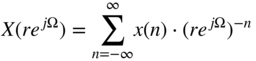
of a discrete‐time system. For a given signal ![]() , we can give its discrete‐time Fourier transform as
, we can give its discrete‐time Fourier transform as
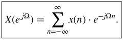
The discrete‐time Fourier Transform describes a spectral transform from the discrete‐time domain ![]() to the frequency domain
to the frequency domain ![]() which is called the Fourier spectrum or Fourier transform of
which is called the Fourier spectrum or Fourier transform of ![]() . The inverse discrete‐time Fourier transform is given by
. The inverse discrete‐time Fourier transform is given by

which takes the discrete‐time Fourier spectrum ![]() and reconstructs the input
and reconstructs the input ![]() . In the following, useful discrete‐time Fourier transform pairs are listed in Eqs. (1.47)–(1.56). An important relation between the time domain
. In the following, useful discrete‐time Fourier transform pairs are listed in Eqs. (1.47)–(1.56). An important relation between the time domain ![]() , using
, using ![]() and
and ![]() giving
giving ![]() , and the frequency domain
, and the frequency domain ![]() , using
, using ![]() and
and ![]() giving
giving ![]() , shows that convolution in the time domain can be described by multiplication in the frequency domain.
, shows that convolution in the time domain can be described by multiplication in the frequency domain.
Discrete‐time Fourier Transform Pairs

1.5 Discrete‐time Fourier Transform and Z‐Transform
The extension of the discrete‐time Fourier transform to the Z‐transform allows for the transform of signals and impulse responses where the discrete‐time Fourier transform does not converge but the Z‐transform converges for a given convergence region. This extension of the discrete‐time Fourier transform

is achieved by introducing a radius ![]() to the complex exponential
to the complex exponential ![]() according to a new complex variable
according to a new complex variable ![]() , which then gives
, which then gives

and thus the Z‐transform

The Z‐transform of many signals leads to a rational function ![]() , with a numerator polynomial
, with a numerator polynomial ![]() and a denominator polynomial
and a denominator polynomial ![]() in the variable
in the variable ![]() . The zeros of the numerator
. The zeros of the numerator ![]() are called the zeros of
are called the zeros of ![]() and the zeros of
and the zeros of ![]() are called the poles of
are called the poles of ![]() . The rational function
. The rational function ![]() can be given in polynomial, pole/zero, and partial expansion forms.
can be given in polynomial, pole/zero, and partial expansion forms.
1.6 Discrete Fourier Transform
To reduce the the length of the input signal ![]() to
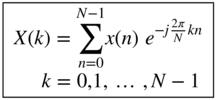
to ![]() samples and to compute the Fourier spectrum only at a finite number of
samples and to compute the Fourier spectrum only at a finite number of ![]() frequency samples, we can discretize the unit circle
frequency samples, we can discretize the unit circle ![]() at
at ![]() frequency samples, and using
frequency samples, and using ![]() samples,
samples, ![]() gives
gives

and the discrete Fourier transform (DFT)
and the inverse discrete Fourier transform (IDFT)

The DFT of a causal audio signal is shown in Fig. 1.9.
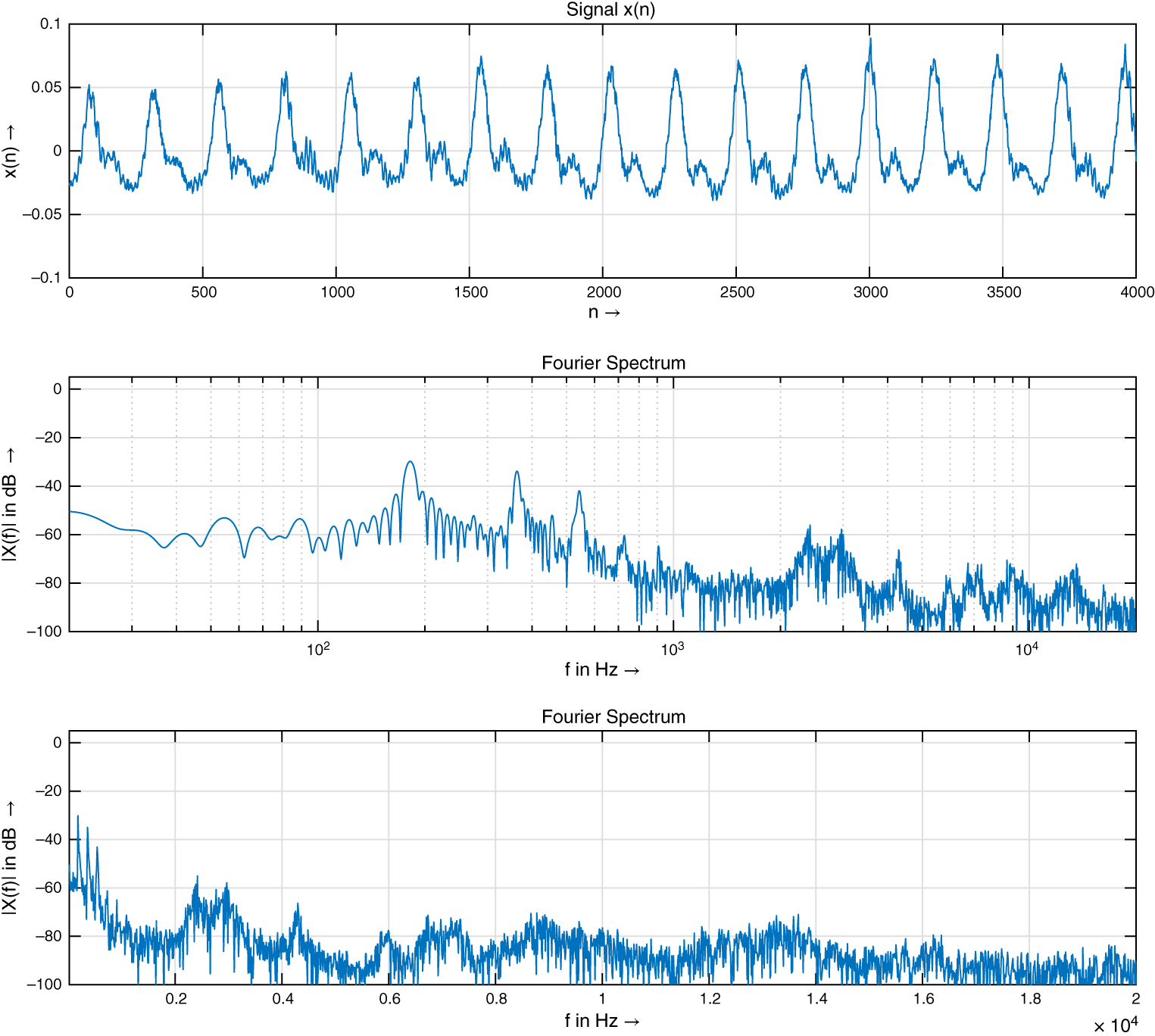
Figure 1.9 Fourier transform of an audio signal  (top plot) and its magnitude spectrum
  in dB versus logarithmic (middle plot) and linear frequency axis (bottom plot).
1.7 FIR and IIR Filters
For causal signals ![]() and causal impulse responses
and causal impulse responses ![]() , the convolution sum is given by
, the convolution sum is given by ![]() . A further simplification is possible if the impulse response is decaying very rapidly and can be truncated in length after
. A further simplification is possible if the impulse response is decaying very rapidly and can be truncated in length after ![]() samples, which then leads to a finite impulse response (FIR) filter with
samples, which then leads to a finite impulse response (FIR) filter with ![]() taps (Matlab file y=filter(b,1,x)) and the discrete‐time convolution
taps (Matlab file y=filter(b,1,x)) and the discrete‐time convolution

which is also called a difference equation. The difference equation can be represented by an FIR signal flow graph (block diagram), as shown in Fig. 1.10. The coefficients ![]() correspond to the impulse response
correspond to the impulse response ![]() . Deriving the Z‐transform of Eq. (1.64) gives
. Deriving the Z‐transform of Eq. (1.64) gives

Figure 1.10 Block diagram of FIR filter.

from which we can derive the system transfer function ![]() , which gives
, which gives

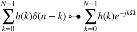
The frequency response of the FIR filter (Matlab file freqz(b,1)) can be derived by taking the discrete‐time Fourier transform of the impulse response or evaluating the system transfer function on the unit circle by replacing ![]() , which gives
, which gives

Figure 1.11 shows a symmetric FIR impulse response with five taps, the magnitude response, phase response, and the pole/zero plot.
If the impulse response is decaying infinitely long, we have an infinite impulse response (IIR) filter of order ![]() (Matlab file y=filter(b,[1 a],x)) which is dependent on its input
(Matlab file y=filter(b,[1 a],x)) which is dependent on its input ![]() and
and ![]() delayed versions
delayed versions ![]() , weighted by the coefficients
, weighted by the coefficients ![]() , and
, and ![]() delayed versions
delayed versions ![]() of the output
of the output ![]() , weighted by the coefficients
, weighted by the coefficients ![]() according to
according to
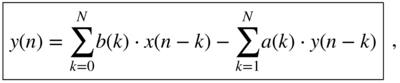
which is also called a difference equation. The difference equation can be represented by an IIR signal flow graph (block diagram), as shown in Fig. 1.12. Performing the Z‐transform of the recursive difference equation in Eq. (1.68) gives

from which we can derive the system transfer function ![]() by deriving
by deriving
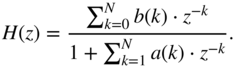
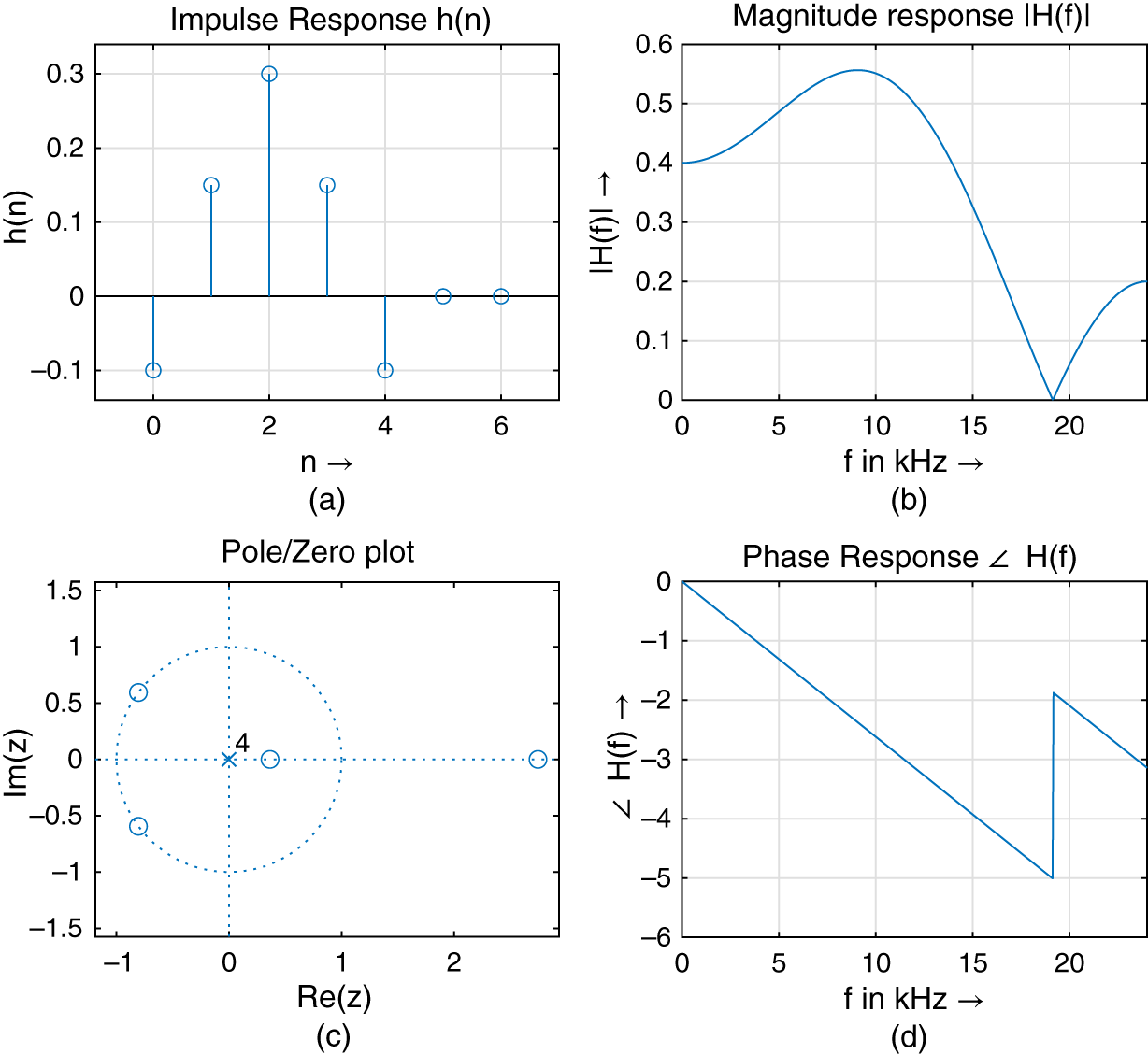
Figure 1.11 FIR filter impulse response, magnitude response, phase response, and pole/zero plot.
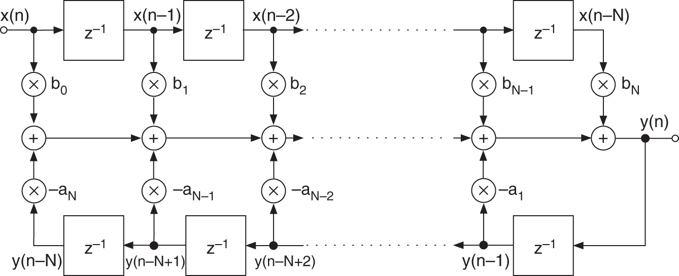
Figure 1.12 Block diagram of an IIR filter.
Typically, ![]() or
or ![]() , and for higher order, we can use a cascade of first‐ and second‐order sub‐filters. Figure 1.13 shows a signal flow graph for an IIR filter cascade. The frequency response of the IIR filter (freqz(b,[1 a])) can be derived by evaluating the system transfer function on the unit circle by replacing
, and for higher order, we can use a cascade of first‐ and second‐order sub‐filters. Figure 1.13 shows a signal flow graph for an IIR filter cascade. The frequency response of the IIR filter (freqz(b,[1 a])) can be derived by evaluating the system transfer function on the unit circle by replacing ![]() , which gives the frequency response of an IIR filter of order
, which gives the frequency response of an IIR filter of order ![]() (freqz(b,[1 a])) according to
(freqz(b,[1 a])) according to
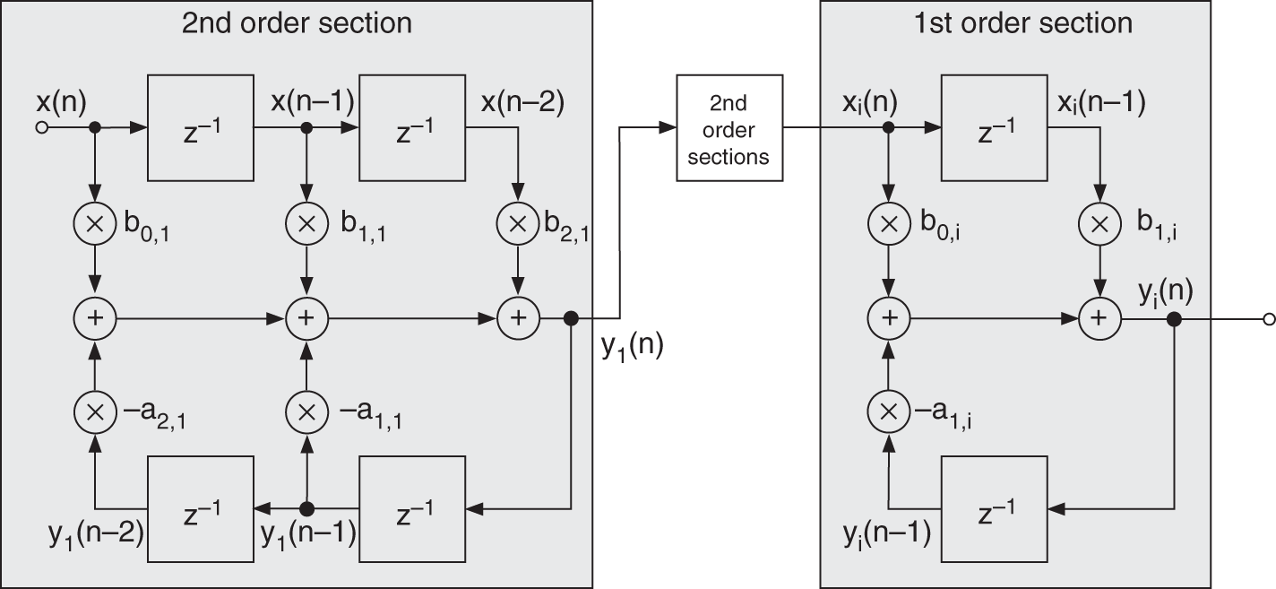
Figure 1.13 IIR filter cascade.

Figure 1.14 shows an IIR impulse response with infinite decay, the magnitude response, phase response, and the pole/zero plot.
Some specific FIR filters are the ![]() ‐tap moving average filter,
‐tap moving average filter,

the triangular filter,
and the equi‐ripple Parks–McClellan filter,

where the impulse response is computed based on the Parks–McClellan [Opp14] design approach. Complementary filters, according to

allow for the use of a lowpass FIR filter of odd length ![]() to perform lowpass‐to‐highpass and bandpass‐to‐bandstop transformations. Some frequency responses of these FIR filters are shown in Fig. 1.15.
to perform lowpass‐to‐highpass and bandpass‐to‐bandstop transformations. Some frequency responses of these FIR filters are shown in Fig. 1.15.
Some simple but effective first‐ and second‐order IIR filters for lowpass (LP), highpass (HP), and bandpass (BP) filtering are given by


Figure 1.14 IIR filter and impulse response, magnitude response, phase response, and pole/zero plot.

Figure 1.15 Frequency responses and impulse responses of a moving average FIR and a Parks–McClellan FIR filter. In the two frequency response plots, a complementary frequency response is also shown.


They all have one (LP, HP) or two coefficients (BP) for controlling their cutoff frequency ![]() in Hz (
in Hz (![]() ‐dB magnitude of LP or HP frequency response) and the BP bandwidth
‐dB magnitude of LP or HP frequency response) and the BP bandwidth ![]() in Hz (lower and higher than
in Hz (lower and higher than ![]() ‐dB magnitude of BP frequency response). Their frequency responses are shown in Fig. 1.16. These simple first‐ and second‐order IIR filters (LP, HP, and BP) can be further implemented using first‐ and second‐order allpass filters
‐dB magnitude of BP frequency response). Their frequency responses are shown in Fig. 1.16. These simple first‐ and second‐order IIR filters (LP, HP, and BP) can be further implemented using first‐ and second‐order allpass filters ![]() and
and ![]() , as shown in the sequence of system transfer functions given by
, as shown in the sequence of system transfer functions given by
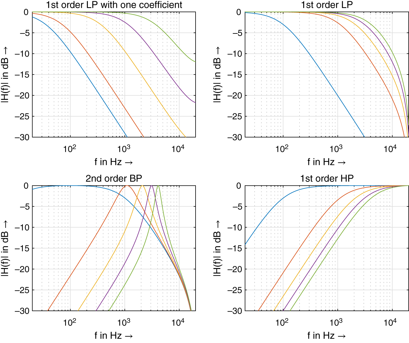
Figure 1.16 Frequency response of IIR filter.


where the coefficients ![]() and
and ![]() are given by Eq. (1.81) and Eq. (1.82), respectively. The lowpass transfer function in Eq. (1.85) is an additive parallel connection of direct path and a first‐order allpass of Eq. (1.83). The highpass transfer function in Eq. (1.86) is a subtractive parallel connection of direct path and a first‐order allpass of Eq. (1.83). Finally, the bandpass transfer function in Eq. (1.87) is a subtractive parallel connection of direct path and a first‐order allpass of Eq. (1.84).
are given by Eq. (1.81) and Eq. (1.82), respectively. The lowpass transfer function in Eq. (1.85) is an additive parallel connection of direct path and a first‐order allpass of Eq. (1.83). The highpass transfer function in Eq. (1.86) is a subtractive parallel connection of direct path and a first‐order allpass of Eq. (1.83). Finally, the bandpass transfer function in Eq. (1.87) is a subtractive parallel connection of direct path and a first‐order allpass of Eq. (1.84).
1.8 Adaptive Filters
Adaptive filters change their filter characteristic according to a predefined error criterion. A generic structure is shown in Fig. 1.17 where a desired signal ![]() is approximated by a reference signal
is approximated by a reference signal ![]() passing through an adaptive filter giving an output signal
passing through an adaptive filter giving an output signal ![]() , which should be made close to
, which should be made close to ![]() such that the error signal
such that the error signal ![]() between the desired signal
between the desired signal ![]() and the output signal
and the output signal ![]() gets smaller with time. The coefficients of the adaptive filter are derived by minimizing the error energy. Based on the generic structure shown in Fig. 1.17, special adaptive filter approaches for system identification, inverse filtering, echo cancellation, and linear prediction can be achieved. We will show how to perform linear prediction as an adaptive FIR filter technique and derive the adaption of the filter coefficients by the autocorrelation method and the least‐mean‐square (LMS) method.
gets smaller with time. The coefficients of the adaptive filter are derived by minimizing the error energy. Based on the generic structure shown in Fig. 1.17, special adaptive filter approaches for system identification, inverse filtering, echo cancellation, and linear prediction can be achieved. We will show how to perform linear prediction as an adaptive FIR filter technique and derive the adaption of the filter coefficients by the autocorrelation method and the least‐mean‐square (LMS) method.

Figure 1.17 Adaptive signal approximation.
Adaptive Linear Prediction using the Autocorrelation Method
For the task of adaptive linear prediction, the generic structure is simplified because the desired signal ![]() is equal to the input
is equal to the input ![]() , which leads to the signal flow graph of linear prediction shown in Fig. 1.18. The adaptive filter is, in that case, an FIR filter with
, which leads to the signal flow graph of linear prediction shown in Fig. 1.18. The adaptive filter is, in that case, an FIR filter with ![]() coefficients. Linear prediction computes an estimate
coefficients. Linear prediction computes an estimate

Figure 1.18 Linear prediction.
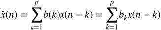
of the actual sample ![]() by a linear combination of past weighted input samples. Here
by a linear combination of past weighted input samples. Here ![]() is the prediction order and
is the prediction order and ![]() are the prediction coefficients. The difference between
are the prediction coefficients. The difference between ![]() and its prediction
and its prediction ![]() is called the prediction error and is given by
is called the prediction error and is given by

The filter coefficients ![]() are computed by minimizing a cost function
are computed by minimizing a cost function
and thus minimizing the quadratic error2. The partial derivatives of the cost function with respect to the filter coefficients ![]() (for
(for ![]() ) lead to
) lead to


Computing the filter coefficients ![]() by setting the partial derivative to zero gives, for
by setting the partial derivative to zero gives, for ![]() ,
,


By using the autocorrelation sequence

and the properties

leads to the set of equations (1.95) in matrix form as
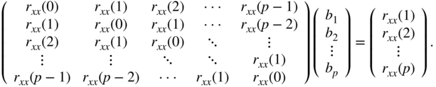
These equations are called Wiener–Hopf equations or normal equations. The so‐called autocorrelation matrix ![]() is symmetric and has identical values on each diagonal. It is a Toeplitz matrix and the set of equations can be solved efficiently by the Levinson–Durbin recursion. The described procedure is called the autocorrelation method for updating the prediction coefficients.
is symmetric and has identical values on each diagonal. It is a Toeplitz matrix and the set of equations can be solved efficiently by the Levinson–Durbin recursion. The described procedure is called the autocorrelation method for updating the prediction coefficients.
Adaptive Linear Prediction using the LMS Method
In this method, a recursive algorithm for minimizing a simplified cost function ![]() is applied by minimizing the LMS error. All filter coefficients will be updated every sampling cycle based on previous values. This recursive approach for the filter coefficients uses the gradient descent formula
is applied by minimizing the LMS error. All filter coefficients will be updated every sampling cycle based on previous values. This recursive approach for the filter coefficients uses the gradient descent formula

with gradient weight ![]() . Using the simplified cost function (instantaneous value of the quadratic error)
. Using the simplified cost function (instantaneous value of the quadratic error)

leads to

and thus, for ![]() , the recursive LMS algorithm
, the recursive LMS algorithm
The gradient weight ![]() can be adjusted using the different LMS approaches listed in Table 1.1.
can be adjusted using the different LMS approaches listed in Table 1.1.
Table 1.1 Computing the gradient weight ![]() .
.
| Standard LMS | |
|---|---|
| Normalized LMS (NLMS) |  |
| Power Normalized (PNLMS) | |
| ‐ Limitation: | |
| ‐ Recursive computation: | |
Linear Prediction for Coding and Source‐filter Processing
Linear prediction can be found in coding and source‐filter processing which have the same signal flow graph of operation, as shown in Fig. 1.19. The first part is the coding operation and consists of a forward prediction and coefficient calculation using the autocorrelation or LMS method. The coder transfer function is given by
Then the error signal ![]() is quantized for the coding application and further processed for source‐filter modifications. The receiver performs a decoding operation by inverse filtering using the prediction filter and the corresponding coefficients from the coder or processed and modified coefficients. The decoder transfer function is given by
is quantized for the coding application and further processed for source‐filter modifications. The receiver performs a decoding operation by inverse filtering using the prediction filter and the corresponding coefficients from the coder or processed and modified coefficients. The decoder transfer function is given by
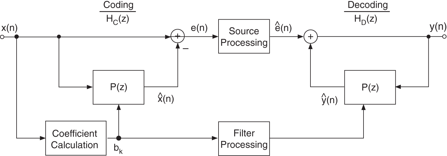
Figure 1.19 Linear prediction for coding and source‐filter processing.
Source‐filter processing extracts, in the time domain, the source signal ![]() through linear prediction and simultaneously the filter coefficients
through linear prediction and simultaneously the filter coefficients ![]() of the prediction filter
of the prediction filter ![]() . The source signal is a whitened version of the input and the filter transfer function
. The source signal is a whitened version of the input and the filter transfer function ![]() represents the spectral envelope of the input
represents the spectral envelope of the input ![]() . Both the source signal
. Both the source signal ![]() and the prediction coefficients
and the prediction coefficients ![]() can be modified according to specific tasks like sound morphing (keeping the source signal and modifying the spectral envelope).
can be modified according to specific tasks like sound morphing (keeping the source signal and modifying the spectral envelope).
1.9 Exercises
1. Signals and Systems
- Sketch the impulse responses:
 (amplifier);
 (delay by
  samples);
 (2‐tap moving average, simple lowpass filter);
 (
( ‐tap moving average, simple lowpass filter);
 (lowpass filter);
 (lowpass filter);
and compute
 for
for  using convolution (folding the impulse response and folding the input signal. Write a Matlab script for the computation of
  .
. - Compute the output signals:
 (eigen signal passing through system);
 (first‐order lowpass filter);
 (integrator);
 (differentiator);
for
 and plot the output signals for
  using Matlab.
2. Discrete‐time Fourier Transform
- Compute the discrete‐time Fourier transform of:
 ;
; ;
; ;
; ;
;
and plot the results using Matlab.
- Using the difference equation

- sketch the signal flow graph;
- compute the frequency response
 ;
; - plot the magnitude response and phase response using Matlab;
- program the difference equation and plot the impulse response.
3. FIR and IIR Filters
- FIR filters with linear phase (even and odd symmetry, linear phase, constant group delay):
 ;
; ;
; ;
; .
.
Plot the impulse responses, magnitude and phase responses (freqz.m), pole/zero plots (zplane.m), and group delay (grpdelay.m). Discuss the results.
- Use FIR filters to approximate a given impulse response by truncating the length of the impulse response to
 taps.
taps. - Do experimentation with the Parks–McClellan design (firpm.m) and design several lowpass filters with linear phase. Use the Matlab files freqz.m and zplane.m for your evaluation.
- Show the IIR signal flow graphs of first‐order LP and HP filters, and second‐order BP filters. Verify the frequency responses.
4. Adaptive Filters
- Write a small script for linear prediction using the LMS algorithm. Use an audio signal and experiment with the prediction order and monitor the error.
- Modify the linear prediction approach by replacing
 , where
  is the unknown system impulse response. Modify the code to perform system identification using the LMS algorithm.
References
- [Opp14] A.V. Oppenheim, A.S. Willsky, with H. Nawab: Signals and Systems, Pearson New International Edition, 2nd Edition, 2014.
- [Opp10] A.V. Oppenheim, R.W. Schafer, with J.R. Buck: Discrete‐time Signal Processing, Prentice Hall Signal Processing Series, 3rd Edition, 2010.