
Chapter 2
Quantization
U. Zölzer
Basic operations for analog‐to‐digital (AD) conversion of a continuous‐time signal ![]() are the sampling and quantization of
are the sampling and quantization of ![]() yielding the quantized sequence
yielding the quantized sequence ![]() (see Fig. 2.1). Before discussing AD/digital‐to‐analog (DA) conversion techniques and the choice of the sampling frequency
(see Fig. 2.1). Before discussing AD/digital‐to‐analog (DA) conversion techniques and the choice of the sampling frequency ![]() in Chapter 3, we will introduce the quantization of the samples
in Chapter 3, we will introduce the quantization of the samples ![]() with a finite number of bits. The digitization of a sampled signal with continuous amplitude is called quantization. The effects of quantization, starting with the classical quantization model, are discussed in Section 2.1. In Section 2.2, dither techniques are presented which, for low‐level signals, linearize the process of quantization. In Section 2.3, spectral shaping of quantization errors is described. Section 2.4 deals with number representation for digital audio signals and their effects on algorithms.
with a finite number of bits. The digitization of a sampled signal with continuous amplitude is called quantization. The effects of quantization, starting with the classical quantization model, are discussed in Section 2.1. In Section 2.2, dither techniques are presented which, for low‐level signals, linearize the process of quantization. In Section 2.3, spectral shaping of quantization errors is described. Section 2.4 deals with number representation for digital audio signals and their effects on algorithms.
2.1 Signal Quantization
2.1.1 Classical Quantization Model
Quantization is described by Widrow's quantization theorem [Wid61]. It says that a quantizer can be modeled (see Fig. 2.2) as the addition of a uniformly distributed random signal ![]() to the original signal
to the original signal ![]() (see Fig. 2.2, [Wid61]). This additive model given by
(see Fig. 2.2, [Wid61]). This additive model given by
is based on the difference between quantized output and input according to the error signal
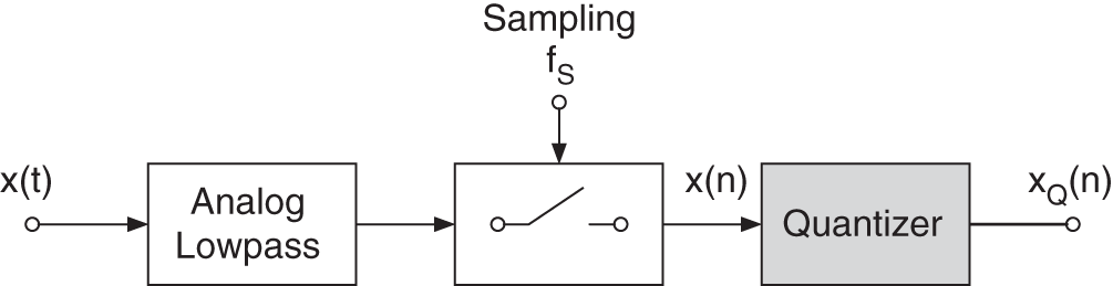
Figure 2.1 AD conversion and quantization.
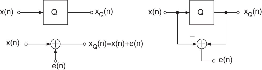
Figure 2.2 Quantization.
This linear model of the output ![]() is only then valid when the input amplitude has a wide dynamic range and the quantization error
is only then valid when the input amplitude has a wide dynamic range and the quantization error ![]() is not correlated with the signal
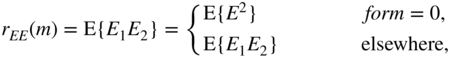
is not correlated with the signal ![]() . Owing to the statistical independence of consecutive quantization errors, the autocorrelation of the error signal is given by
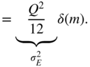
. Owing to the statistical independence of consecutive quantization errors, the autocorrelation of the error signal is given by ![]() , which yields a power density spectrum
, which yields a power density spectrum ![]() .
.
The nonlinear process of quantization is described by a nonlinear characteristic curve, as shown in Fig. 2.3a, where ![]() denotes the quantization step. The difference between output and input of the quantizer provides the quantization error
denotes the quantization step. The difference between output and input of the quantizer provides the quantization error ![]() , which is shown in Fig. 2.3b. The uniform probability density function (PDF) of the quantization error is given (see Fig. 2.3b) by
, which is shown in Fig. 2.3b. The uniform probability density function (PDF) of the quantization error is given (see Fig. 2.3b) by
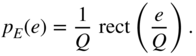
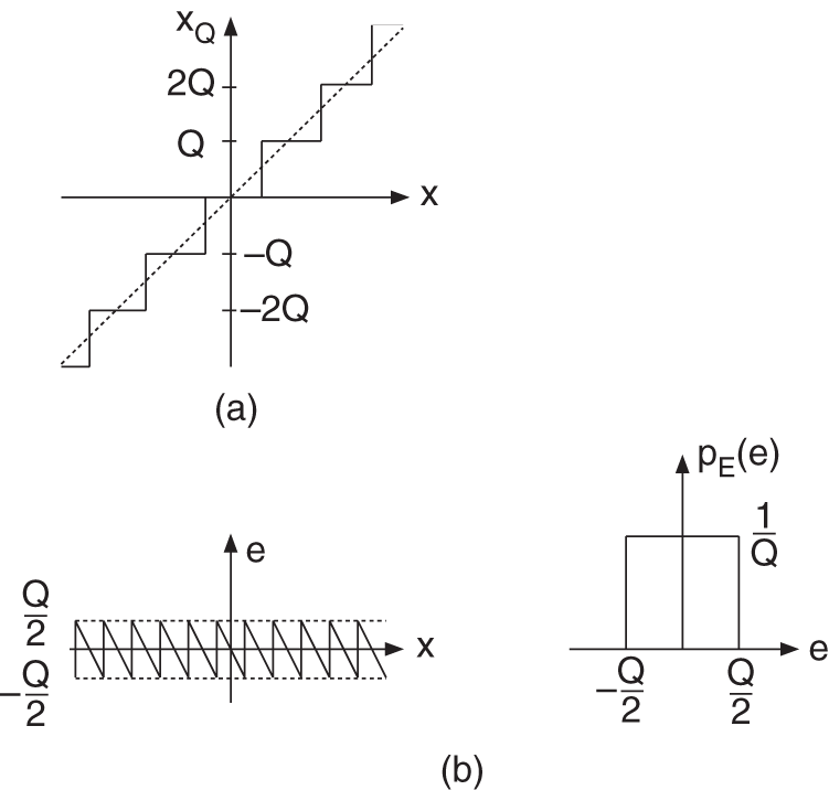
Figure 2.3 (a) Nonlinear characteristic curve of a quantizer. (b) Quantization error  and its probability density function (PDF)
  .
.
The ![]() th moment of a random variable
th moment of a random variable ![]() with a PDF
with a PDF ![]() is defined as the expected value of
is defined as the expected value of ![]() :
:

For a uniformly distributed random process, as in Eq. (2.3), the first two moments are given by

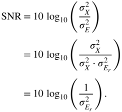
The signal‐to‐noise ratio (SNR)
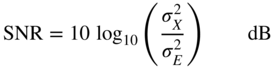
is defined as the ratio of signal power ![]() to error power
to error power ![]() .
.
For a quantizer with input range ![]() and word length
and word length ![]() , the quantization step size can be expressed as
, the quantization step size can be expressed as
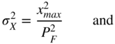
By defining a peak factor
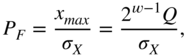
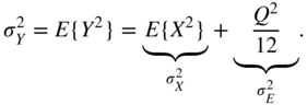
the variances of the input and the quantization error can be written as

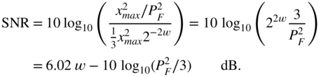
The SNR is then given by
A sinusoidal signal (PDF as in Fig. 2.4) with ![]() gives
gives
For a signal with uniform PDF (see Fig. 2.4) and ![]() , we can write
, we can write
and for a Gaussian distributed signal (probability of overload ![]() leads to
leads to ![]() , see Fig. 2.5), it follows that
, see Fig. 2.5), it follows that

Figure 2.4 Probability density function (sinusoidal signal and signal with uniform PDF).
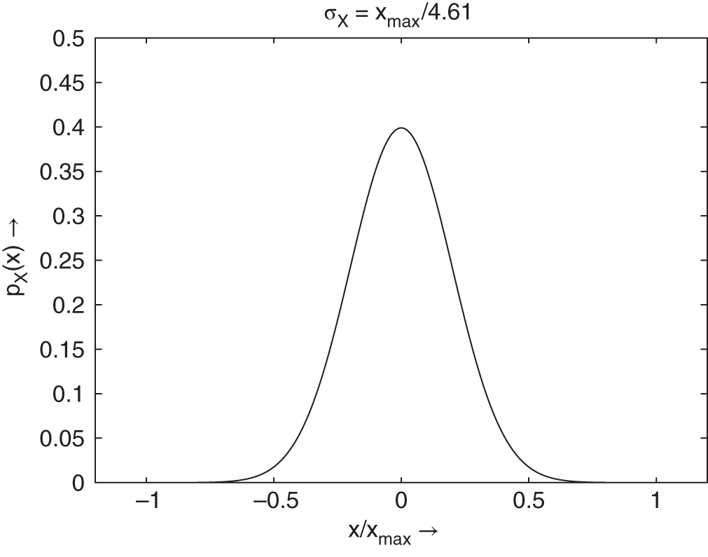
Figure 2.5 Probability density function (signal with Gaussian PDF).
It is obvious that the SNR depends on the PDF of the input. For digital audio signals that exhibit nearly Gaussian distribution, the maximum SNR for a given word length ![]() is 8.5 dB lower than the rule of thumb formula (2.14) for the SNR.
is 8.5 dB lower than the rule of thumb formula (2.14) for the SNR.
2.1.2 Quantization Theorem
The statement of the quantization theorem for amplitude sampling (digitizing the amplitude) of signals has been given by Widrow [Wid61]. The analogy for digitizing the time axis is the sampling theorem given by Shannon [Sha48]. Figure 2.6 shows the amplitude quantization and the time quantization. First of all, the PDF of the output signal of a quantizer is determined in terms of the PDF of the input signal. Both PDFs are shown in Fig. 2.7. The respective characteristic functions (Fourier transform of a PDF) of the input and output signals form the basis for Widrow's quantization theorem.
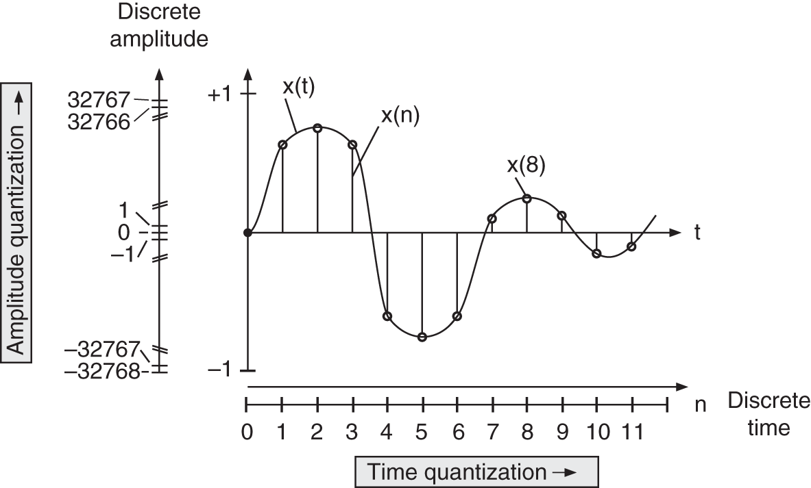
Figure 2.6 Amplitude and time quantization.

Figure 2.7 Probability density function of signal  and quantized signal
  .
.
First‐order Statistics of the Quantizer Output
Quantization of a continuous‐amplitude signal ![]() with PDF
with PDF ![]() leads to a discrete‐amplitude signal
leads to a discrete‐amplitude signal ![]() with PDF
with PDF ![]() (see Fig. 2.8). The continuous PDF of the input is sampled by integrating over all quantization intervals (zone sampling). This leads to a discrete PDF of the output.
(see Fig. 2.8). The continuous PDF of the input is sampled by integrating over all quantization intervals (zone sampling). This leads to a discrete PDF of the output.
In the quantization intervals, the discrete PDF of the output is determined by the probability
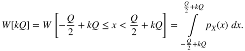
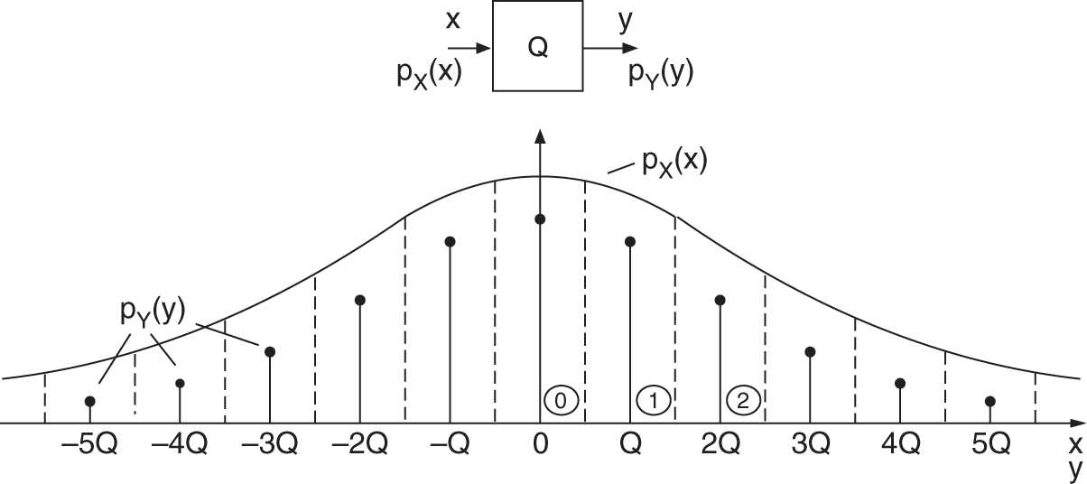
Figure 2.8 Zone sampling of the PDF.
For the intervals ![]() , it follows that
, it follows that
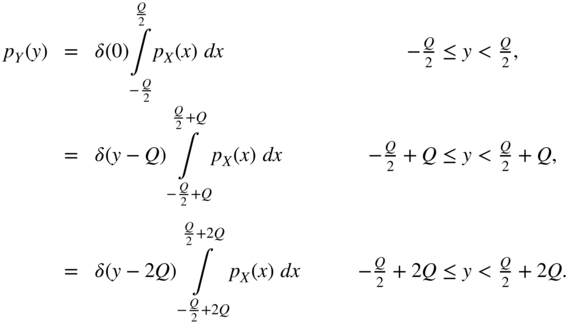
The summation over all intervals gives the PDF of the output
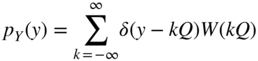

where
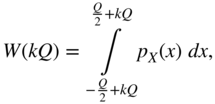

Using

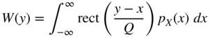
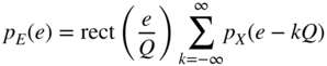
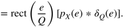
the PDF of the output is given by
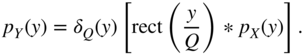
Hence, the PDF of the output can be determined by convolution of a rect function [Lip92] with the PDF of the input. This is followed by an amplitude sampling with resolution ![]() as described in Eq. (2.23) (see Fig. 2.9).
as described in Eq. (2.23) (see Fig. 2.9).
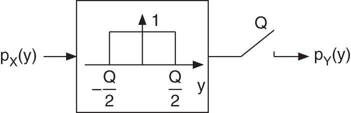
Figure 2.9 Determining the PDF of the output.
Using ![]() , the characteristic function (Fourier transform of
, the characteristic function (Fourier transform of ![]() ) can be written as
) can be written as
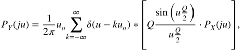

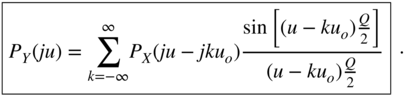
Equation (2.26) describes the sampling of the continuous PDF of the input. If the quantization frequency ![]() is twice the highest frequency of the characteristic function
is twice the highest frequency of the characteristic function ![]() , then periodically recurring spectra do not overlap. Hence, a reconstruction of the PDF of the input
, then periodically recurring spectra do not overlap. Hence, a reconstruction of the PDF of the input ![]() from the quantized PDF of the output
from the quantized PDF of the output ![]() is possible (see Fig. 2.10). This is known as the quantization theorem of Widrow. In contrast to the first sampling theorem (Shannon's sampling theorem, ideal amplitude sampling in the time domain)
is possible (see Fig. 2.10). This is known as the quantization theorem of Widrow. In contrast to the first sampling theorem (Shannon's sampling theorem, ideal amplitude sampling in the time domain) ![]() , it can be observed that there is an additional multiplication of the periodically characteristic function with
, it can be observed that there is an additional multiplication of the periodically characteristic function with 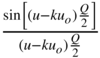 (see Eq. (2.26)).
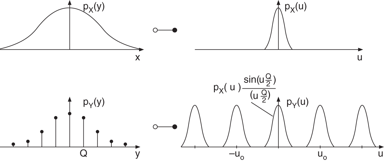
Figure 2.10 Spectral representation.
If the baseband of the characteristic function (![]() )
)
is considered, it is observed that it is a product of two characteristic functions. The multiplication of characteristic functions leads to the convolution of PDFs, from which the addition of two statistically independent signals can be concluded. Hence, the characteristic function of the quantization error is
and the PDF
(see Fig. 2.11).

Figure 2.11 PDF and characteristic function of quantization error.
The modeling of the quantization process as an addition of a statistically independent noise signal to the input signal leads to a continuous PDF of the output (see Fig. 2.12, convolution of PDFs and sampling in the interval ![]() gives the discrete PDF of the output). The PDF of the discrete‐valued output comprises Dirac pulses at distance
gives the discrete PDF of the output). The PDF of the discrete‐valued output comprises Dirac pulses at distance ![]() with values equal to the continuous PDF (see Eq. (2.23)). Only if the quantization theorem is valid, the continuous PDF can be reconstructed from the discrete PDF.
with values equal to the continuous PDF (see Eq. (2.23)). Only if the quantization theorem is valid, the continuous PDF can be reconstructed from the discrete PDF.

Figure 2.12 PDF of the model.
In many cases, it is not necessary to reconstruct the PDF of the input. It is sufficient to calculate the moments of the input from the output. The ![]() th moment can be expressed in terms of the PDF or the characteristic function:
th moment can be expressed in terms of the PDF or the characteristic function:
If the quantization theorem is satisfied, then the periodic terms in Eq. (2.26) do not overlap and the ![]() th derivative of
th derivative of ![]() is solely determined by the baseband1 so that with Eq. (2.26), it can be written
is solely determined by the baseband1 so that with Eq. (2.26), it can be written

With Eq. (2.32), the first two moments can be determined as
Second‐order Statistics of Quantizer Output
To describe the properties of the output in the frequency domain, two output values ![]() (at time
(at time ![]() ) and
) and ![]() (at time
(at time ![]() ) are considered [Lip92]. For the joint density function,
) are considered [Lip92]. For the joint density function,
with
and

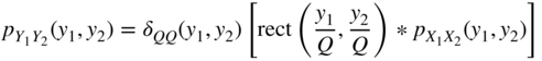
For the two‐dimensional Fourier transform, it follows that
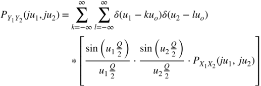
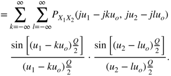
Similar to the one‐dimensional quantization theorem, a two‐dimensional theorem [Wid61] can be formulated: the joint density function of the input can be reconstructed from the joint density function of the output, if ![]() for
for ![]() and
and ![]() . Here again, the moments of the joint density function can be calculated as follows:
. Here again, the moments of the joint density function can be calculated as follows:
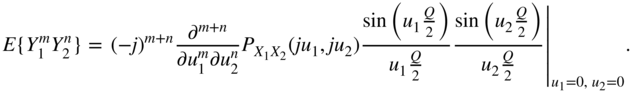
From this, the autocorrelation function with ![]() can be written as
can be written as
(for ![]() , we obtain Eq. (2.34)).
, we obtain Eq. (2.34)).
2.1.3 Statistics of Quantization Error
First‐order Statistics of Quantization Error
The PDF of the quantization error depends on the PDF of the input and is dealt with in the following. The quantization error ![]() is restricted to the interval
is restricted to the interval ![]() . It depends linearly on the input (see Fig. 2.13). If the input value lies in the interval
. It depends linearly on the input (see Fig. 2.13). If the input value lies in the interval ![]() , then the error is
, then the error is ![]() . For the PDF, we obtain
. For the PDF, we obtain ![]() . If the input value lies in the interval
. If the input value lies in the interval ![]() , then the quantization error is
, then the quantization error is ![]() and is again restricted to
and is again restricted to ![]() . The PDF of the quantization error is consequently
. The PDF of the quantization error is consequently ![]() and is added to the first term. For the sum over all intervals, we can write
and is added to the first term. For the sum over all intervals, we can write
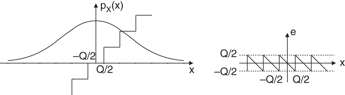
Figure 2.13 Probability density function and quantization error.

Because of the restricted values of the variable of the PDF, we can write
The PDF of the quantization error is determined by the PDF of the input and can be computed by shifting and windowing a zone. All individual zones are summed up for calculating the PDF of the quantization error [Lip92]. A simple graphical interpretation of this overlapping is shown in Fig. 2.14. The overlapping leads to a uniform distribution of the quantization error if the input PDF ![]() is spread over a sufficient number of quantization intervals.
is spread over a sufficient number of quantization intervals.
For the Fourier transform of the PDF from Eq. (2.44) follows


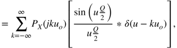
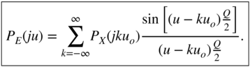
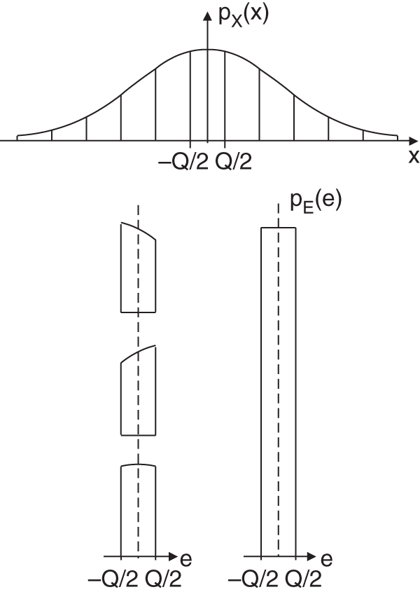
Figure 2.14 Probability density function of the quantization error.
If the quantization theorem is satisfied, i.e. if ![]() for
for ![]() , then there is only one non‐zero term (
, then there is only one non‐zero term (![]() in Eq. (2.48)). The characteristic function of the quantization error is reduced, with
in Eq. (2.48)). The characteristic function of the quantization error is reduced, with ![]() , to
, to

Hence, the PDF of the quantization error is

Sripad and Snyder [Sri77] have modified the sufficient condition of Widrow (band‐limited characteristic function of input) for a quantization error of uniform PDF by the weaker condition

The uniform distribution of the input PDF

with characteristic function

does not satisfy Widrow's condition for a band‐limited characteristic function, but instead the weaker condition

is fulfilled. From this follows the uniform PDF in Eq. (2.49) of the quantization error. The weaker condition from Sripad and Snyder extends the class of input signals for which a uniform PDF of the quantization error can be assumed.
To show the deviation from the uniform PDF of the quantization error as a function of the PDF of the input, Eq. (2.48) can be written as

The inverse Fourier transform yields


Equation (2.56) shows the effect of the input PDF on the deviation from a uniform PDF.
Second‐order Statistics of Quantization Error
For describing the spectral properties of the error signal, two values ![]() (at time
(at time ![]() ) and
) and ![]() (at time
(at time ![]() ) are considered [Lip92]. The joint PDF is given by
) are considered [Lip92]. The joint PDF is given by

Here ![]() and
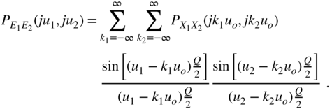
and ![]() . For the Fourier transform of the joint PDF, a similar procedure to that shown by (Eqs. 2.45)–(2.48) leads to
. For the Fourier transform of the joint PDF, a similar procedure to that shown by (Eqs. 2.45)–(2.48) leads to
If the quantization theorem and/or the Sripad–Snyder condition
are satisfied, then

For the joint PDF of the quantization error, it then holds that

Owing to the statistical independence of quantization errors (Eq. (2.63)),
For the moments of the joint PDF,

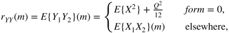
From this, it follows for the autocorrelation function with ![]()

The power density spectrum of the quantization error is then given by
which is equal to the variance ![]() of the quantization error (see Fig. 2.15).
of the quantization error (see Fig. 2.15).

Figure 2.15 Autocorrelation  and power density spectrum
  of quantization error
  .
.
Correlation of Signal and Quantization Error
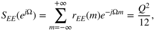
For describing the correlation of the signal and the quantization error [Sri77], the second moment of the output with Eq. (2.26) is derived as follows:


With the quantization error ![]() ,
,
where the term ![]() , with Eq. (2.72), is written as
, with Eq. (2.72), is written as

With the assumption of a Gaussian PDF of the input, we obtain
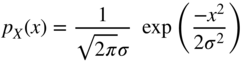
with the characteristic function

Using Eq. (2.57), the PDF of the quantization error is then given by
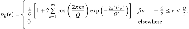
Figure 2.16a shows the PDF in Eq. (2.77) of the quantization error for different variances of the input.
For the mean value and the variance of a quantization error, it follows from Eq. (2.77) that ![]() and
and


Figure 2.16 (a) Probability density function of quantization error for different standard deviations of a Gaussian PDF input. (b) Variance of quantization error for different standard deviations of a Gaussian PDF input.
Figure 2.16b shows the variance of the quantization error in Eq. (2.78) for different variances of the input.
For a Gaussian PDF input, as given by (Eqs. 2.75) and (2.76), the correlation (see Eq. (2.74)) between input and quantization error is expressed as

The correlation is negligible for large values of ![]() .
.
2.2 Dither
2.2.1 Basics
The requantization (renewed quantization of already quantized signals) to limited word lengths occurs repeatedly during storage, format conversion, and signal processing algorithms. Here, small signal levels lead to error signals which depend on the input. Owing to quantization, nonlinear distortion occurs for low‐level signals. The conditions for the classical quantization model are not satisfied anymore. To reduce these effects for signals of small amplitude, a linearization of the nonlinear characteristic curve of the quantizer is performed. This is done by adding a random sequence ![]() to the quantized signal
to the quantized signal ![]() (see Fig. 2.17) before the actual quantization process. The specification of the word length is shown in Fig. 2.18. This random signal is called dither. The statistical independence of the error signal from the input is not achieved, but the conditional moments of the error signal can be affected [Lip92, Ger89, Wan92, Wan00].
(see Fig. 2.17) before the actual quantization process. The specification of the word length is shown in Fig. 2.18. This random signal is called dither. The statistical independence of the error signal from the input is not achieved, but the conditional moments of the error signal can be affected [Lip92, Ger89, Wan92, Wan00].
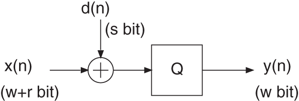
Figure 2.17 Addition of a random sequence before a quantizer.
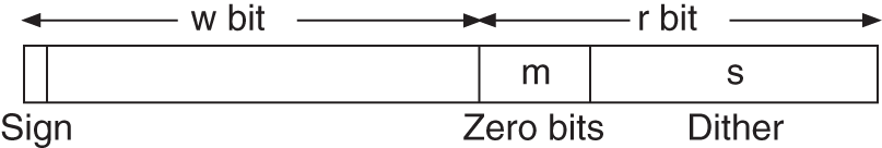
Figure 2.18 Specification of the word length.
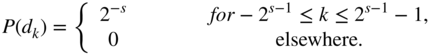
The sequence ![]() , with amplitude range (
, with amplitude range (![]() ), is generated with the help of a random number generator and is added to the input. For a dither value with
), is generated with the help of a random number generator and is added to the input. For a dither value with ![]() :
:
The index ![]() of the random number
of the random number ![]() characterizes the value from the set of
characterizes the value from the set of ![]() possible numbers with the probability
possible numbers with the probability
With the mean value ![]() , the variance
, the variance ![]() , and the quadratic mean
, and the quadratic mean ![]() , we can rewrite the variance as
, we can rewrite the variance as ![]() .
.
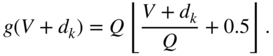
For a static input amplitude ![]() and the dither value
and the dither value ![]() , the rounding operation [Lip86] is expressed as
, the rounding operation [Lip86] is expressed as
For the mean of the output ![]() as a function of the input
as a function of the input ![]() , we can write
, we can write
The quadratic mean of the output ![]() for input
for input ![]() is given by
is given by
For the variance ![]() for input
for input ![]() ,
,
The above‐mentioned equations have the input ![]() as a parameter. Figures 2.19 and 2.20 illustrate the mean output
as a parameter. Figures 2.19 and 2.20 illustrate the mean output ![]() and the standard deviation
and the standard deviation ![]() within a quantization step size, which are given by (Eqs. 2.83), (2.84), and (2.85). The examples of rounding and truncation demonstrate the linearization of the characteristic curve of the quantizer. The coarse step size is replaced by a finer one. The quadratic deviation from the mean output
within a quantization step size, which are given by (Eqs. 2.83), (2.84), and (2.85). The examples of rounding and truncation demonstrate the linearization of the characteristic curve of the quantizer. The coarse step size is replaced by a finer one. The quadratic deviation from the mean output ![]() is termed noise modulation. For a uniform PDF dither, this noise modulation depends on the amplitude (see Figs. 2.19 and 2.20). It is maximum in the middle of the quantization step size and approaches zero towards the end. The linearization and the suppression of the noise modulation can be achieved by a triangular PDF dither with bipolar characteristic [Van89] and rounding operation (see Fig. 2.20). Triangular PDF dither is obtained by adding two statistically independent dither signals with uniform PDF (convolution of PDFs). A dither signal with a higher‐order PDF is not necessary for audio signals [Lip92, Wan00].
is termed noise modulation. For a uniform PDF dither, this noise modulation depends on the amplitude (see Figs. 2.19 and 2.20). It is maximum in the middle of the quantization step size and approaches zero towards the end. The linearization and the suppression of the noise modulation can be achieved by a triangular PDF dither with bipolar characteristic [Van89] and rounding operation (see Fig. 2.20). Triangular PDF dither is obtained by adding two statistically independent dither signals with uniform PDF (convolution of PDFs). A dither signal with a higher‐order PDF is not necessary for audio signals [Lip92, Wan00].
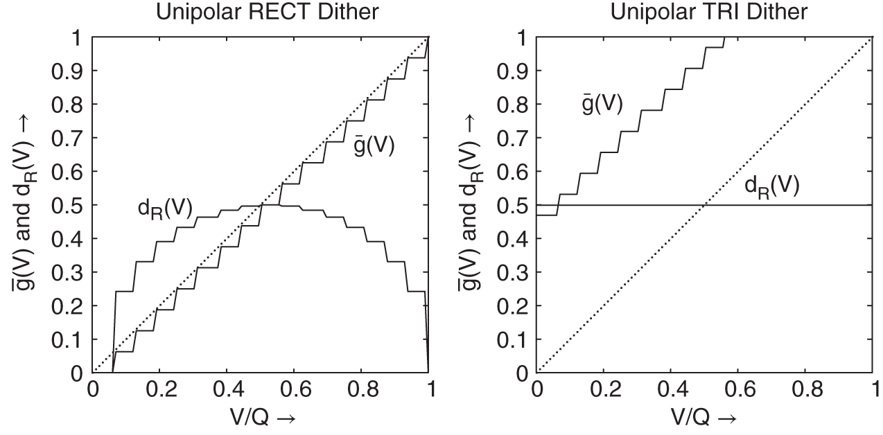
Figure 2.19 Truncation – linearizing and suppression of noise modulation ( ,
,  ).
).

Figure 2.20 Rounding – linearizing and suppression of noise modulation ( ,
,  ).
).
The total noise power for this quantization technique consists of the dither power and the power of the quantization error [Lip86]. The following noise powers are obtained by integration with respect to ![]() as follows.
as follows.
- Mean dither power
 :
(2.86)
:
(2.86)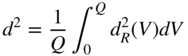 (2.87)
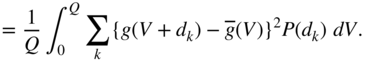
(This is equal to the deviation from mean output in accordance with Eq. (2.83).)
- Mean of total noise power
 :
:
(This is equal to the deviation from an ideal straight line.)
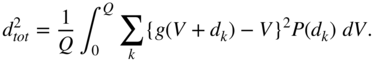
To derive a relationship between ![]() and
and ![]() , the quantization error given by
, the quantization error given by
is used to rewrite Eq. (2.88) as

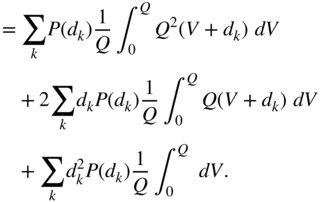
The integrals in Eq. (2.91) are independent of ![]() . Moreover,
. Moreover, ![]() . With the mean value of the quantization error
. With the mean value of the quantization error
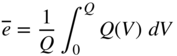
and the quadratic mean error
it is possible to rewrite Eq. (2.91) as
With ![]() and
and ![]() , Eq. (2.94) can be written as
, Eq. (2.94) can be written as
Equations (2.94) and (2.95) describe the total noise power as a function of the quantization (![]() ) and the dither addition (
) and the dither addition (![]() ). It can be seen that for zero‐mean quantization, the middle term in Eq. (2.95) results in
). It can be seen that for zero‐mean quantization, the middle term in Eq. (2.95) results in ![]() . The acoustically perceptible part of the total error power is represented by
. The acoustically perceptible part of the total error power is represented by ![]() and
and ![]() .
.
2.2.2 Implementation
The random sequence ![]() is generated with the help of a random number generator with uniform PDF. For generating a triangular PDF random sequence, two independent uniform PDF random sequences
is generated with the help of a random number generator with uniform PDF. For generating a triangular PDF random sequence, two independent uniform PDF random sequences ![]() and
and ![]() can be added. To generate a triangular highpass dither, the dither value
can be added. To generate a triangular highpass dither, the dither value ![]() is added to
is added to ![]() . Thus, only one random number generator is required. In conclusion, the following dither sequences can be implemented:
. Thus, only one random number generator is required. In conclusion, the following dither sequences can be implemented:
The power density spectra of triangular PDF dither and triangular PDF HP dither are shown in Fig. 2.21. Figure 2.22 shows histograms of a uniform PDF dither and a triangular PDF highpass dither together with their respective power density spectra. The amplitude range of a uniform PDF dither lies between ![]() , whereas it lies between
, whereas it lies between ![]() for triangular PDF dither. The total noise power for triangular PDF dither is doubled.
for triangular PDF dither. The total noise power for triangular PDF dither is doubled.

Figure 2.21 Normalized power density spectrum for triangular PDF dither (TRI) with  and triangular PDF highpass dither (HP) with
  .
.
2.2.3 Examples
The effect of the input amplitude of the quantizer is shown in Fig. 2.23 for a 16‐bit quantizer (![]() ). A quantized sinusoidal signal with amplitude
). A quantized sinusoidal signal with amplitude ![]() (one‐bit amplitude) and frequency
(one‐bit amplitude) and frequency ![]() is shown in Fig. 2.23a,b for rounding and truncation. Figure 2.23c,d shows their corresponding spectra. For truncation, Fig. 2.23c shows the spectral line of the signal and the spectral distribution of the quantization error with the harmonics of the input signal. For rounding, Fig. 2.23d shows that, with special signal frequency
is shown in Fig. 2.23a,b for rounding and truncation. Figure 2.23c,d shows their corresponding spectra. For truncation, Fig. 2.23c shows the spectral line of the signal and the spectral distribution of the quantization error with the harmonics of the input signal. For rounding, Fig. 2.23d shows that, with special signal frequency ![]() , the quantization error is concentrated in uneven harmonics.
, the quantization error is concentrated in uneven harmonics.

Figure 2.22 (a,d) Histogram and (c,d) power density spectrum of uniform PDF dither (RECT) with  and triangular PDF highpass dither (HP) with
  .
.
In the following, only the rounding operation is used. By adding a uniform PDF random signal to the actual signal before quantization, the quantized signal shown in Fig. 2.24a results. The corresponding power density spectrum is illustrated in Fig. 2.24c. In the time domain, it is observed that the one‐bit amplitudes approach zero so that the regular pattern of the quantized signal is affected. The resulting power density spectrum in Fig. 2.24c shows that the harmonics do not occur anymore and the noise power is uniformly distributed over the frequencies. For triangular PDF dither, the quantized signal is shown in Fig. 2.24b. Owing to triangular PDF, amplitudes of ![]() occur in addition to the signal values of
occur in addition to the signal values of ![]() and zero. Figure 2.24d shows the increase of the total noise power.
and zero. Figure 2.24d shows the increase of the total noise power.
To illustrate the noise modulation for uniform PDF dither, the amplitude of the input is reduced to ![]() and the frequency is chosen as
and the frequency is chosen as ![]() . This means that the input amplitude to the quantizer is 0.25 bit. For a quantizer without additive dither, the quantized output signal is zero. For RECT dither, the quantized signal is shown in Fig. 2.25a. The input signal with amplitude
. This means that the input amplitude to the quantizer is 0.25 bit. For a quantizer without additive dither, the quantized output signal is zero. For RECT dither, the quantized signal is shown in Fig. 2.25a. The input signal with amplitude ![]() is also shown. The power density spectrum of the quantized signal is shown in Fig. 2.25c. The spectral line of the signal and the uniform distribution of the quantization error can be seen. However, in the time domain, a correlation between positive and negative amplitudes of the input and the quantized positive and negative values of the output can be observed. In hearing tests, this noise modulation occurs if the amplitude of the input is decreased continuously and falls below the amplitude of the quantization step. This process occurs for all fade‐out processes that occur in speech and music signals. For positive low‐amplitude signals, two output states zero and Q occur, and for negative low‐amplitude signals, the output states zero and ‐Q occur. This is observed as a disturbing rattle which is overlapped on the actual signal. If the input level is further reduced, the quantized output approaches zero.
is also shown. The power density spectrum of the quantized signal is shown in Fig. 2.25c. The spectral line of the signal and the uniform distribution of the quantization error can be seen. However, in the time domain, a correlation between positive and negative amplitudes of the input and the quantized positive and negative values of the output can be observed. In hearing tests, this noise modulation occurs if the amplitude of the input is decreased continuously and falls below the amplitude of the quantization step. This process occurs for all fade‐out processes that occur in speech and music signals. For positive low‐amplitude signals, two output states zero and Q occur, and for negative low‐amplitude signals, the output states zero and ‐Q occur. This is observed as a disturbing rattle which is overlapped on the actual signal. If the input level is further reduced, the quantized output approaches zero.
Figure 2.23 One‐bit amplitude – quantizer with truncation (a,c) and rounding (b,d).
To reduce this noise modulation at low levels, a triangular PDF dither is used. Figure 2.25b shows the quantized signal and Fig. 2.25d shows the power density spectrum. It can be observed that the quantized signal has an irregular pattern. Hence, a direct association of positive half‐waves with the positive output values, as well as vice versa, is not possible. The power density spectrum shows the spectral line of the signal along with an increase in noise power owing to triangular PDF dither. In acoustic hearing tests, the use of triangular PDF dither results in a constant noise floor even if the input level is reduced to zero.
2.3 Spectrum Shaping of Quantization – Noise Shaping
Using the linear model of a quantizer in Fig. 2.26 and the relations
Figure 2.24 One‐bit amplitude – rounding with RECT dither (a,c) and TRI dither (b,d).
the quantization error ![]() may be isolated and fed back through a transfer function
may be isolated and fed back through a transfer function ![]() , as shown in Fig. 2.27. This leads to the spectral shaping of the quantization error as given by
, as shown in Fig. 2.27. This leads to the spectral shaping of the quantization error as given by
and the corresponding Z‐transforms
A simple spectrum shaping of the quantization error ![]() is achieved by feeding back with
is achieved by feeding back with ![]() , as shown in Fig. 2.28, and leads to
, as shown in Fig. 2.28, and leads to
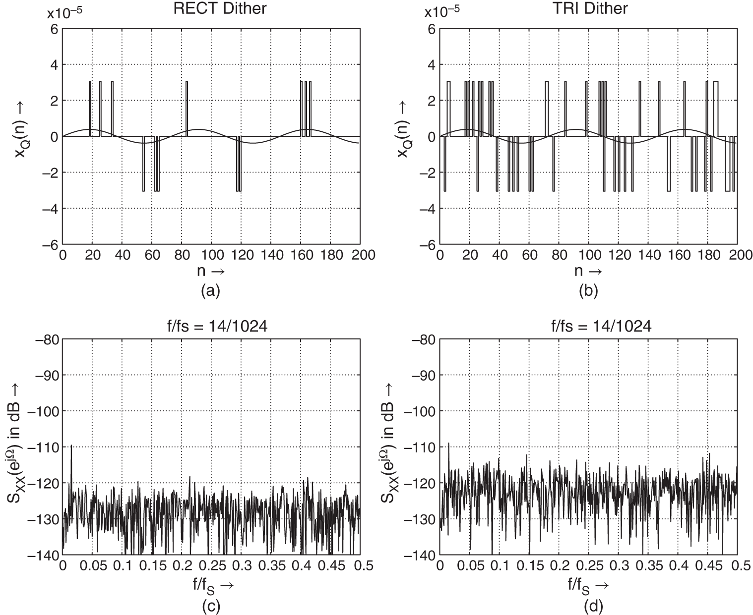
Figure 2.25 Noise modulation at 0.25‐bit amplitude – rounding with RECT dither (a,c) and TRI dither (b,d).
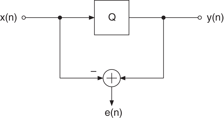
Figure 2.26 Linear model of a quantizer.

Figure 2.27 Spectrum shaping of quantization error.

Figure 2.28 Highpass spectrum shaping of quantization error.
and the Z‐transforms
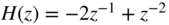
Equation (2.113) shows a highpass weighting of the original error signal ![]() . By choosing
. By choosing ![]() , second‐order highpass weighting given by
, second‐order highpass weighting given by
can be achieved. The power density spectrum of the error signal for the two cases is given by
Figure 2.29 shows the weighting of the power density spectrum by this noise shaping technique.

Figure 2.29 Spectrum shaping ( ,
,  ;
;  , ;
, ;  , ‐ ‐ ‐).
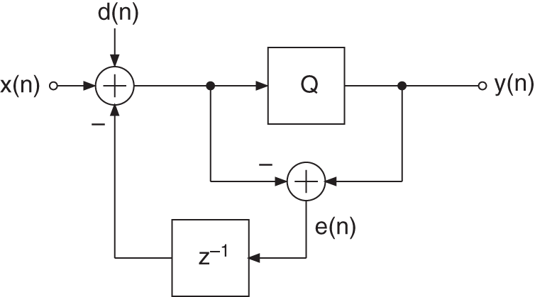
Figure 2.30 Dither and spectrum shaping.
By adding a dither signal ![]() (see Fig. 2.30), the output and the error are given by
(see Fig. 2.30), the output and the error are given by
and
For the Z‐transforms, we write
The modified error signal ![]() consists of the dither and the highpass shaped quantization error.
consists of the dither and the highpass shaped quantization error.
By moving the addition (Fig. 2.31) of the dither directly before the quantizer, a highpass spectrum shaping is obtained for both the error signal and the dither. Here, the following relationships hold:
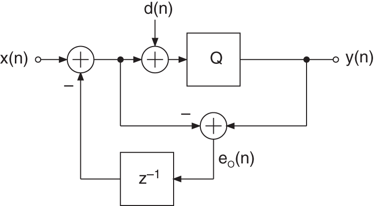
Figure 2.31 Modified dither and spectrum shaping.
with the Z‐transforms given by
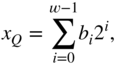
Apart from the discussed feedback structures which are easy to implement on a digital signal processor and which lead to highpass noise shaping, there are psychoacoustic‐based noise‐shaping methods that have been proposed in the literature [Ger89, Wan92, Hel07]. These methods use special approximations of the hearing threshold (threshold in quiet, absolute threshold) for the feedback structure ![]() . Figure 2.32a shows several hearing threshold models as a function of frequency [ISO389, Ter79, Wan92]. It can be seen that the sensitivity of human hearing is high for frequencies between 2 and 6 kHz and sharply decreases for high and low frequencies. Figure 2.32b also shows the inverse ISO 389‐7 threshold curve, which represents an approximation of the filtering operation in our perception. The feedback filter of the noise shaper should affect the quantization error with the inverse ISO389 weighting curve. Hence, the noise power in the frequency range with high sensitivity should be reduced and shifted toward lower and higher frequencies. Figure 2.33a shows the unweighted power density spectra of the quantization error for three special filters
. Figure 2.32a shows several hearing threshold models as a function of frequency [ISO389, Ter79, Wan92]. It can be seen that the sensitivity of human hearing is high for frequencies between 2 and 6 kHz and sharply decreases for high and low frequencies. Figure 2.32b also shows the inverse ISO 389‐7 threshold curve, which represents an approximation of the filtering operation in our perception. The feedback filter of the noise shaper should affect the quantization error with the inverse ISO389 weighting curve. Hence, the noise power in the frequency range with high sensitivity should be reduced and shifted toward lower and higher frequencies. Figure 2.33a shows the unweighted power density spectra of the quantization error for three special filters ![]() [Wan92, Hel07]. Figure 2.33b depicts the same three power density spectra, weighted by the inverse ISO 389 threshold of Fig. 2.32b. These weighted power density spectra (PDS) show that the perceived noise power is reduced by all three noise shapers versus the frequency axis. Figure 2.34 shows a sinusoid with amplitude
[Wan92, Hel07]. Figure 2.33b depicts the same three power density spectra, weighted by the inverse ISO 389 threshold of Fig. 2.32b. These weighted power density spectra (PDS) show that the perceived noise power is reduced by all three noise shapers versus the frequency axis. Figure 2.34 shows a sinusoid with amplitude ![]() , which is quantized to
, which is quantized to ![]() bit with psychoacoustic noise shaping. The quantized signal
bit with psychoacoustic noise shaping. The quantized signal ![]() consists of different amplitudes reflecting the low‐level signal. The power density spectrum of the quantized signal reflects the psychoacoustic weighting of the noise shaper with a fixed filter. A time‐variant psychoacoustic noise shaping is described in [DeK03, Hel07], where the instantaneous masking threshold is used for adaptation of a time‐variant filter.
consists of different amplitudes reflecting the low‐level signal. The power density spectrum of the quantized signal reflects the psychoacoustic weighting of the noise shaper with a fixed filter. A time‐variant psychoacoustic noise shaping is described in [DeK03, Hel07], where the instantaneous masking threshold is used for adaptation of a time‐variant filter.
2.4 Number Representation
The different applications in digital signal processing and transmission of audio signals lead to the question of the type of number representation for digital audio signals. In this section, basic properties of fixed‐point and floating‐point number representation in the context of digital audio signal processing are presented.

Figure 2.32 (a) Hearing thresholds in quiet. (b) Inverse ISO 389‐7 threshold curve.
2.4.1 Fixed‐point Number Representation
In general, an arbitrary real number ![]() can be approximated by a finite summation
can be approximated by a finite summation
where the possible values for ![]() are 0 and 1.
are 0 and 1.
The fixed‐point number representation with a finite number ![]() of binary places leads to four different interpretations of the number range (see Table 2.1 and Fig. 2.35).
of binary places leads to four different interpretations of the number range (see Table 2.1 and Fig. 2.35).
The signed fractional representation (2s complement) is the usual format for digital audio signals and for algorithms in fixed‐point arithmetic. For address and modulo operation, the unsigned integer is used. Owing to finite word length ![]() , overflow occurs, as shown in Fig. 2.36. These curves have to be taken into consideration while carrying out operations, especially additions in 2s complement arithmetic.
, overflow occurs, as shown in Fig. 2.36. These curves have to be taken into consideration while carrying out operations, especially additions in 2s complement arithmetic.
Quantization is carried out with techniques, as shown in Table 2.2, for rounding and truncation. The quantization step size is characterized by ![]() and the symbol
and the symbol ![]() denotes the biggest integer smaller than or equal to
denotes the biggest integer smaller than or equal to ![]() . Figure 2.37 shows the rounding and truncation curves for 2s complement number representation. The absolute error shown in Fig. 2.37 is given by
. Figure 2.37 shows the rounding and truncation curves for 2s complement number representation. The absolute error shown in Fig. 2.37 is given by ![]() .
.
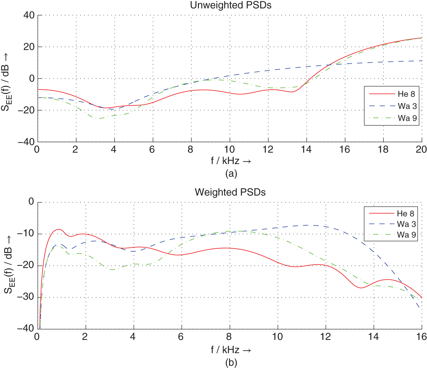
Figure 2.33 Power density spectra of three filter approximations (Wa3, third‐order filter; Wa9, ninth‐order filter; He8, eighth‐order filter [Wan92, Hel07]): (a) unweighted power spectral densities (PSDs); (b) inverse ISO 389‐7 weighted PSDs.
Table 2.1 Bit location and range of values.
| Type | Bit location | Range of values | ||
|---|---|---|---|---|
| Signed 2s c. | ||||
| Unsigned 2s c. | 0 | |||
| Signed int. | ||||
| Unsigned int. | 0 | |||
Digital audio signals are coded in the 2s complement number representation. For 2s complement representation, the range of values from ![]() to
to ![]() is normalized to the range −1 to +1 and is represented by the weighted finite sum
is normalized to the range −1 to +1 and is represented by the weighted finite sum ![]() . The variables
. The variables ![]() to
to ![]() are called bits and can take the values 1 or 0. The bit
are called bits and can take the values 1 or 0. The bit ![]() is called MSB (most significant bit) and
is called MSB (most significant bit) and ![]() is called LSB (least significant bit). For positive numbers,
is called LSB (least significant bit). For positive numbers, ![]() is equal to 0 and for negative numbers,
is equal to 0 and for negative numbers, ![]() equals 1. For a three‐bit quantization (see Fig. 2.38), a quantized value can be represented by
equals 1. For a three‐bit quantization (see Fig. 2.38), a quantized value can be represented by ![]() . The smallest quantization step size is 0.25. For a positive number 0.75, it follows that
. The smallest quantization step size is 0.25. For a positive number 0.75, it follows that ![]() . The binary coding for 0.75 is 011.
. The binary coding for 0.75 is 011.

Figure 2.34 Psychoacoustic noise shaping: signal  ; quantized signal
  ; and power density spectrum of quantized signal.
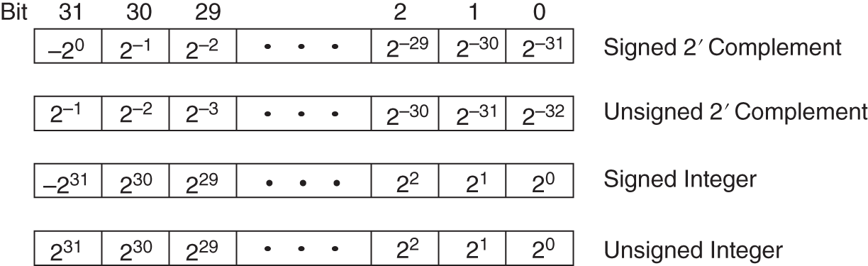
Figure 2.35 Fixed‐point formats.
Dynamic Range. The dynamic range of a number representation is defined as the ratio of maximum to minimum number. For fixed‐point representation with

Figure 2.36 Number range.

Figure 2.37 Rounding and truncation curves.
Table 2.2 Rounding and truncation of 2s complement numbers.
| Type | Quantization | Error limits | ||
|---|---|---|---|---|
| 2s c. (r) | ||||
| 2s c. (t) | 0 | |||
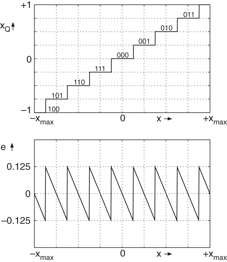
Figure 2.38 Rounding curve and error signal for  bit.
bit.
the dynamic range is given by

Multiplication and Addition of Fixed‐point Numbers. For the multiplication of two fixed‐point numbers in the range from ![]() to
to ![]() , the result is always less than 1. For the addition of two fixed‐point numbers, care must be taken for the result to remain in the range from
, the result is always less than 1. For the addition of two fixed‐point numbers, care must be taken for the result to remain in the range from ![]() to
to ![]() . An addition of
. An addition of ![]() must be carried out in the form
must be carried out in the form ![]() . This multiplication by the factor 0.5 or generally
. This multiplication by the factor 0.5 or generally ![]() is called scaling. An integer in the range from one to, for instance, eight is chosen for the scaling coefficient
is called scaling. An integer in the range from one to, for instance, eight is chosen for the scaling coefficient ![]() .
.
Error Model. The quantization process for fixed‐point numbers can be approximated as an addition of an error signal ![]() to the signal
to the signal ![]() (see Fig. 2.39). The error signal is a random signal with white power density spectrum.
(see Fig. 2.39). The error signal is a random signal with white power density spectrum.
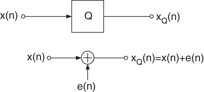
Figure 2.39 Model of a fixed‐point quantizer.
Signal‐to‐noise Ratio. The SNR for a fixed‐point quantizer is defined by

where ![]() is the signal power and
is the signal power and ![]() is the noise power.
is the noise power.
2.4.2 Floating‐point Number Representation
The representation of a floating‐point number is given by
with
where ![]() denotes the normalized mantissa and
denotes the normalized mantissa and ![]() the exponent. The normalized standard format (IEEE) is shown in Fig. 2.40 and special cases are given in Table 2.3. The mantissa
the exponent. The normalized standard format (IEEE) is shown in Fig. 2.40 and special cases are given in Table 2.3. The mantissa ![]() is implemented with a word length of
is implemented with a word length of ![]() bits and is in fixed‐point number representation. The exponent
bits and is in fixed‐point number representation. The exponent ![]() is implemented with a word length of
is implemented with a word length of ![]() bits and is an integer in the range from
bits and is an integer in the range from ![]() to
to ![]() . For an exponent word length of
. For an exponent word length of ![]() bits, its range of values is between
bits, its range of values is between ![]() and +127. The range of values of the mantissa is between 0.5 and 1. This is denoted as the normalized mantissa and is responsible for a unique representation of a number. For a fixed‐point number in the range between 0.5 and 1, it follows that the exponent of the floating‐point number representation is
and +127. The range of values of the mantissa is between 0.5 and 1. This is denoted as the normalized mantissa and is responsible for a unique representation of a number. For a fixed‐point number in the range between 0.5 and 1, it follows that the exponent of the floating‐point number representation is ![]() . For representing a fixed‐point number in the range between 0.25 and 0.5 in floating‐point representation, the range of values of the normalized mantissa
. For representing a fixed‐point number in the range between 0.25 and 0.5 in floating‐point representation, the range of values of the normalized mantissa ![]() lies between 0.5 and 1, and for the exponent it follows
lies between 0.5 and 1, and for the exponent it follows ![]() . As an example, for a fixed‐point number 0.75, the floating‐point number
. As an example, for a fixed‐point number 0.75, the floating‐point number ![]() results. The fixed‐point number 0.375 is not represented as the floating‐point number
results. The fixed‐point number 0.375 is not represented as the floating‐point number ![]() . With the normalized mantissa, the floating‐point number is expressed as
. With the normalized mantissa, the floating‐point number is expressed as ![]() . Owing to normalization, ambiguity of the floating‐point number representation is avoided. Numbers
. Owing to normalization, ambiguity of the floating‐point number representation is avoided. Numbers ![]() can be represented. For example, 1.5 becomes
can be represented. For example, 1.5 becomes ![]() in floating‐point number representation.
in floating‐point number representation.
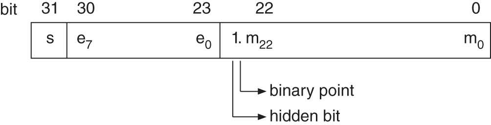
Figure 2.40 Floating‐point number representation.
Table 2.3 Special cases of floating‐point number representation.
| Type | Exponent | Mantissa | Value |
|---|---|---|---|
| NAN | 255 | undefined | |
| Infinity | 255 | 0 | |
| Normal | any | ||
| Zero | 0 | 0 |
Figure 2.41 shows the rounding and truncation curves for floating‐point representation and the absolute error ![]() . The curves for floating‐point quantization show that for small amplitudes, small quantization steps sizes occur. In contrast to fixed‐point representation, the absolute error is dependent on the input signal.
. The curves for floating‐point quantization show that for small amplitudes, small quantization steps sizes occur. In contrast to fixed‐point representation, the absolute error is dependent on the input signal.
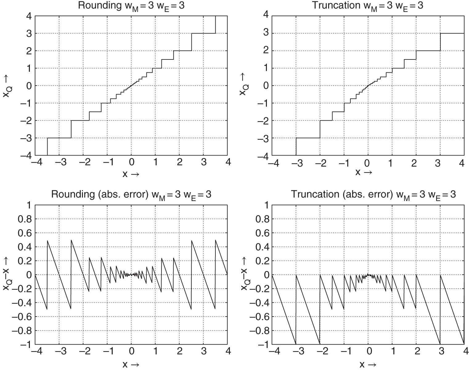
Figure 2.41 Rounding and truncation curves for floating‐point representation.
In the interval
the quantization step is given by
For the relative error
of the floating‐point representation, a constant upper limit can be stated as
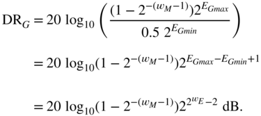
Dynamic Range. With the maximum and minimum numbers given by
and
the dynamic range for floating‐point representation is given by
Multiplication and Addition of Floating‐point Numbers. For multiplications with floating‐point numbers, the exponents of both numbers ![]() and
and ![]() are added and the mantissas are multiplied. The resulting exponent
are added and the mantissas are multiplied. The resulting exponent ![]() is adjusted so that
is adjusted so that ![]() lies in the interval
lies in the interval ![]() . For additions, the smaller number is denormalized to get the same exponent. Then both mantissa are added and the result is normalized.
. For additions, the smaller number is denormalized to get the same exponent. Then both mantissa are added and the result is normalized.
Error Model. With the definition of the relative error ![]() , the quantized signal can be written as
, the quantized signal can be written as
Floating‐point quantization can be modeled as an additive error signal ![]() to the signal
to the signal ![]() (see Fig. 2.42).
(see Fig. 2.42).
Signal‐to‐noise Ratio. Under the assumption that the relative error is independent of the input ![]() , the noise power of the floating‐point quantizer can be written as
, the noise power of the floating‐point quantizer can be written as
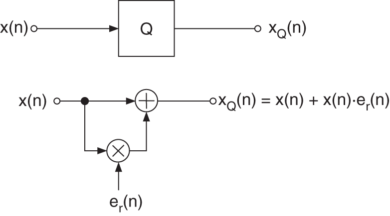
Figure 2.42 Model of a floating‐point quantizer.
For the SNR, we can derive
Equation (2.149) shows that the SNR is independent of the level of the input. It is only dependent on the noise power ![]() which, in turn, is only dependent on the word length
which, in turn, is only dependent on the word length ![]() of the mantissa of the floating‐point representation.
of the mantissa of the floating‐point representation.
2.4.3 Effects on Format Conversion and Algorithms
First, a comparison of the SNR is made for the fixed‐point and floating‐point number representations. Figure 2.43 shows the SNR as a function of input level for both number representations. The fixed‐point word length is ![]() bits. The word length of the mantissa in floating‐point representation is also
bits. The word length of the mantissa in floating‐point representation is also ![]() bits whereas that of the exponent is
bits whereas that of the exponent is ![]() bits The SNR for the floating‐point representation shows that it is independent of input level and varies as a saw‐tooth curve in a 6‐dB grid. If the input level is so low that a normalization of the mantissa arising from finite number representation is not possible, then the SNR is comparable to the fixed‐point representation. While using the full range, both fixed‐point and floating‐point result in the same SNR. It can be noticed that the SNR for the fixed‐point representation depends on the input level. This SNR in the digital domain is an exact image of the level‐dependent SNR of an analog signal in the analog domain. A floating‐point representation cannot improve this SNR. Rather, the floating‐point curve is vertically shifted downwards to the value of the SNR of an analog signal.
bits The SNR for the floating‐point representation shows that it is independent of input level and varies as a saw‐tooth curve in a 6‐dB grid. If the input level is so low that a normalization of the mantissa arising from finite number representation is not possible, then the SNR is comparable to the fixed‐point representation. While using the full range, both fixed‐point and floating‐point result in the same SNR. It can be noticed that the SNR for the fixed‐point representation depends on the input level. This SNR in the digital domain is an exact image of the level‐dependent SNR of an analog signal in the analog domain. A floating‐point representation cannot improve this SNR. Rather, the floating‐point curve is vertically shifted downwards to the value of the SNR of an analog signal.
AD/DA Conversion. Before processing, storing, and transmission of audio signals, the analog audio signal is converted into a digital signal. The precision of this conversion depends on the word length ![]() of the AD converter. The resulting SNR is
of the AD converter. The resulting SNR is ![]() dB for uniform PDF inputs. The SNR in the analog domain depends on the level. This linear dependence of the SNR on the level is preserved after AD conversion with subsequent fixed‐point representation.
dB for uniform PDF inputs. The SNR in the analog domain depends on the level. This linear dependence of the SNR on the level is preserved after AD conversion with subsequent fixed‐point representation.

Figure 2.43 Signal‐to‐noise ratio for an input level.
Equalizers. While implementing equalizers with recursive digital filters, the SNR depends on the choice of the recursive filter structure. By a suitable choice of a filter structure and methods to spectrally shape the quantization errors, optimal SNRs are obtained for a given word length. The SNR for a fixed‐point representation depends on the word length, and for a floating‐point representation on the word length of the mantissa. For filter implementations with fixed‐point arithmetic, boost filters have to be implemented with a scaling within the filter algorithm. The properties of a floating‐point representation take care of automatic scaling in boost filters. If an insert inpit/output (I/O) in fixed‐point representation follows a boost filter in floating‐point representation, then the same scaling as in fixed‐point arithmetics has to be done.
Dynamic Range Control. Dynamic range control is performed by a simple multiplicative weighting of the input signal with a control factor. The latter follows from calculating the peak and root‐mean‐square (RMS) value of the input signal. The number representation of the signal has no influence on the properties of the algorithm. Owing to the normalized mantissa in the floating‐point representation, some simplifications are produced while determining the control factor.
Mixing/Summation. While mixing signals to a stereo image, only multiplications and additions occur. Under the assumption of incoherent signals, an overload reserve can be estimated. This implies a reserve of 20/30 dB for 48/96 sources. For fixed‐point representation, the overload reserve is provided by a number of overflow bits in the accumulator of a digital signal processor (DSP). The properties of automatic scaling in floating‐point arithmetic provide for overload reserves. For both number representations, the summation signal must be matched with the number representation of the output. While dealing with AES/EBU outputs or MADI outputs, both number representations are adjusted to a fixed‐point format. Similarly, within heterogeneous system solutions, it is logical to make heterogeneous use of both number representations though corresponding number representations have to be converted.
Because the SNR in fixed‐point representation depends on the input level, a conversion from fixed‐point to floating‐point representation does not lead to a change of the SNR, i.e. the conversion does not improve the SNR. Further signal processing with floating‐point or fixed‐point arithmetic does not alter the SNR as long as the algorithms are chosen and programmed accordingly. Reconversion from floating‐point to fixed‐point representation again leads to a level‐dependent SNR.
As a consequence, for two‐channel DSP systems which operate with AES/EBU or with analog inputs and outputs, and which are used for equalization, dynamic range control, room simulation etc., the above‐mentioned holds. These conclusions are also valid for digital mixing consoles for which digital inputs from AD converters or from multitrack machines are represented in fixed‐point format (AES/EBU or MADI). The number representation for inserts and auxiliaries is specific to a system. Digital AES/EBU (or MADI) inputs and outputs are realized in fixed‐point number representation.
2.5 JS Applet – Quantization, Dither, and Noise Shaping
This applet shown in Fig. 2.44 demonstrates audio effects resulting from quantization. It is designed as a first insight into the perceptual effects of quantizing an audio signal.
The following functions can be selected on the lower right of the graphical user interface:
- Quantizer
- – word length
 leads to a quantization step size
  ;
;
- – word length
- Dither
- – rect dither – uniform probability density function,
- – tri dither – triangular probability density function,
- – highpass dither – triangular probability density function and highpass power spectral density;
- Noise shaping
- – first‐order
 ,
, - – second‐order
 ,
, - – psychoacoustic noise shaping.
- – first‐order
You can choose between two predefined audio files from our web server (audio1.wav or audio2.wav) or your own local WAV file to be processed [Gui05].
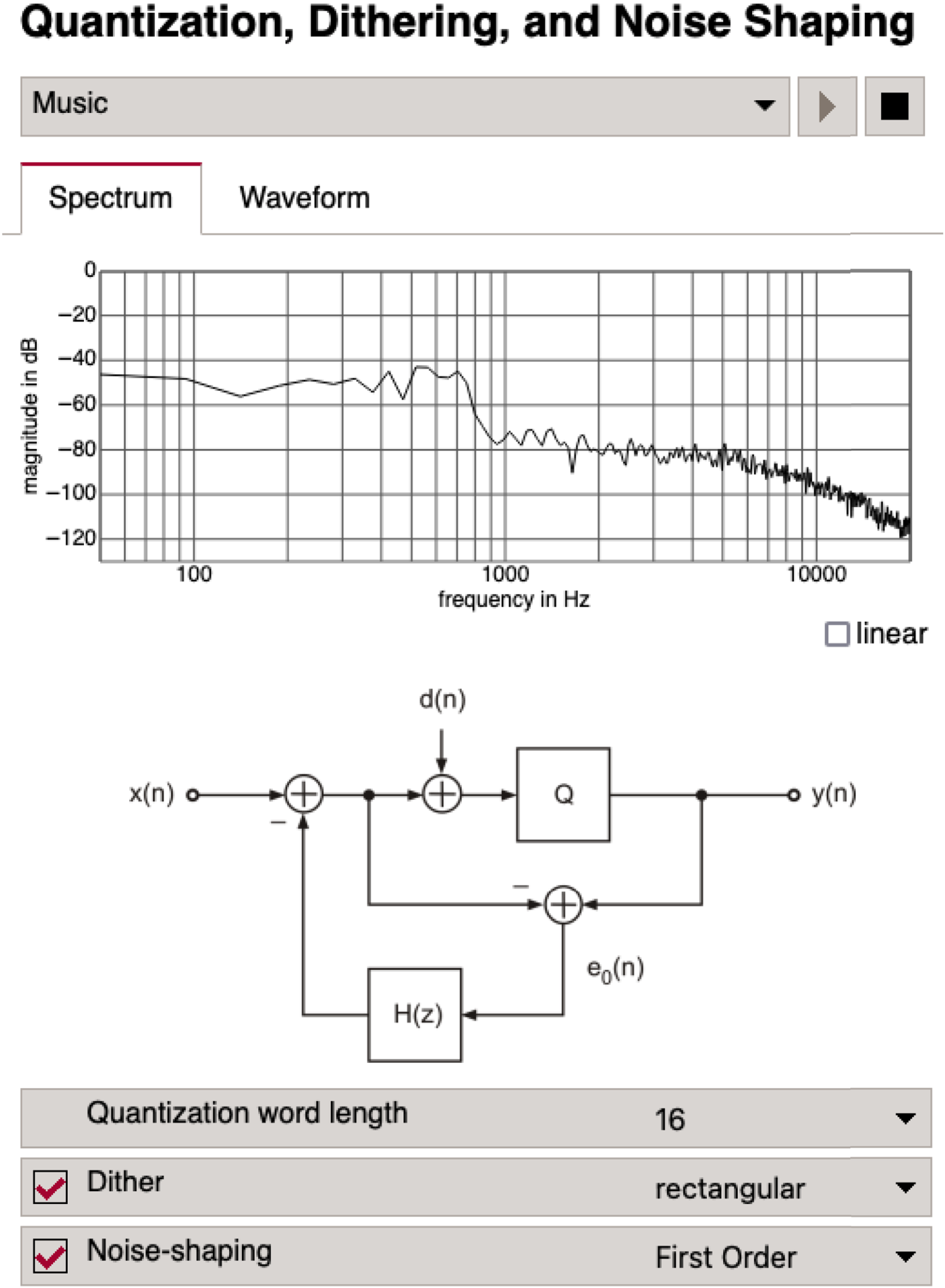
Figure 2.44 JS applet – quantization, dither, and noise shaping.
2.6 Exercises
1. Quantization
- Consider a 100‐Hz sine wave
 sampled with
  kHz,
kHz,  number of samples, and
  bit (word length). What is the number of quantization levels? What is the quantization step
  when the signal is normalized to
  . Show graphically how quantization is performed. What is the maximum error for this 3‐bit quantizer? Write a Matlab code for quantization with rounding and truncation.
 - Derive the mean value, the variance, and the peak factor
 of sequence
  if the signal has a uniform probability density function (PDF) in the range
  . Derive the signal‐to‐noise ratio (SNR) for this case. What will happen if we increase our word length by one bit?
 - As the input signal level decreases from maximum amplitude to very low amplitudes, the error signal becomes more audible. Describe the error calculated above when
 decreases to 1 bit? Is the classical quantization model still valid? What can be done to avoid this distortion?
 - Write a Matlab code for a quantizer with
 bit with rounding and truncation.
- Plot the nonlinear transfer characteristic and the error signal when the input signal covers the range
 .
. - Consider the sine wave
 with
with  and
and  . Plot the output signal (
 ) of a quantizer with rounding and truncation in the time domain and the frequency domain.
 - Compute for both quantization types the quantization error and the SNR.
- Plot the nonlinear transfer characteristic and the error signal when the input signal covers the range
2. Dither
- What is dither and when do we have to use it?
- How do we perform dither and what kinds of dither do we have?
- How do we obtain a triangular highpass dither and why do we prefer it to other dithers?
- Matlab: Generate corresponding dither signals for rectangular, triangular, and triangular highpass.
- Plot the amplitude distribution and the spectrum of the output
 of a quantizer for every dither type.
3. Noise Shaping
- What is noise shaping and when do we do it?
- Why is it necessary to dither during noise shaping and how do we do this?
- Matlab: The first noise shaper used is without dither and assumes that the transfer function in the feedback structure can be first‐order
 or second‐order
  . Plot the output
  and the error signal
  and its spectrum. Show with a plot how the error signal will be shaped.
 - The same noise shaper is now used with a dither signal. Is it really necessary to dither with noise shaping? Where would you add your dither in the flow graph to achieve better results?
- In the feedback structure, we now use a psychoacoustic‐based noise shaper which uses the Wannamaker filter coefficients:

Show with a Matlab plot how the error is shaped by this filter.
References
- [DeK03] D. De Koning, W. Verhelst: On Psychoacoustic Noise Shaping for Audio Requantization, Proc. ICASSP‐03, Vol. 5, pp. 453–456, April 2003.
- [Ger89] M.A. Gerzon, P.G. Craven: Optimal Noise Shaping and Dither of Digital Signals, Proc. 87th AES Convention, New York, Preprint No. 2822, October 1989.
- [Gui05] M. Guillemard, C. Ruwwe, U. Zölzer: J‐DAFx ‐ Digital Audio Effects in Java, Proc. 8th Int. Conference on Digital Audio Effects (DAFx‐05), Madrid, Spain, pp.161–166, 2005.
- [Hel07] C.R. Helmrich, M. Holters, and U. Zölzer, Improved Psychoacoustic Noise Shaping for Requantization of High‐Resolution Digital Audio, AES 31st International Conference, London, UK, June 2007.
- [ISO389]ISO 389‐7:2005, Acoustics – Reference zero for the calibration of audiometric equipment – Part 7: Reference threshold of hearing under free‐field and diffuse‐field listening conditions, Geneva, Switzerland, 2005.
- [Lip86] S.P. Lipshitz, J. Vanderkoy: Digital Dither, Proc. 81st AES Convention, Los Angeles, Preprint No. 2412, November 1986.
- [Lip92] S.P. Lipshitz, R.A. Wannamaker, J. Vanderkoy: Quantization and Dither: A Theoretical Survey, J. Audio Eng. Soc., Vol. 40, No. 5, pp. 355–375, May 1992.
- [Sha48] C.E. Shannon: A Mathematical Theory of Communication, Bell Systems, Techn. J., pp. 379–423, pp. 623–656, 1948.
- [Sri77] A.B. Sripad, D.L. Snyder: A Necessary and Sufficient Condition for Quantization Errors to be Uniform and White, IEEE Trans. ASSP, Vol. 25, pp. 442–448, Oct. 1977.
- [Ter79] E. Terhardt, Calculating Virtual Pitch, Hearing Res., Vol. 1, pp. 155–182, 1979.
- [Van89] J. Vanderkooy, S.P. Lipshitz: Digital Dither: Signal Processing with Resolution Far below the Least Significant Bit, Proc. AES Int. Conf. on Audio in Digital Times, pp. 87–96, May 1989.
- [Wan92] R.A. Wannamaker: Psychoacoustically Optimal Noise Shaping, J. Audio Eng. Soc., Vol. 40, No. 7/8, pp. 611–620, July/August 1992.
- [Wan00] R.A. Wannamaker, S.P. Lipshitz, J. Vanderkooy, J.N. Wright: A Theory of Nonsubtractive Dither, IEEE Trans. Signal Processing, Vol. 48, No. 2, pp. 499–516, 2000.
- [Wid61] B. Widrow: Statistical Analysis of Amplitude‐Quantized Sampled‐Data Systems, Trans. AIEE, Pt. II, Vol. 79, pp. 555–568, Jan. 1961.