
Chapter 7
Room Simulation
U. Zölzer P. Nowak and P. Bhattacharya
Room simulation artificially reproduces the acoustics of a room. The foundations of room acoustics are found in [Cre78, Kut91]. Room simulation is mainly used for post‐processing signals in which a microphone is located in the vicinity of an instrument or a voice. The direct signal, without additional room impression, is mapped to a certain acoustical room, for example, a concert hall or a church. In terms of signal processing, the post‐processing of an audio signal with room simulation corresponds to the convolution of the audio signal with a room impulse response.
7.1 Basics
7.1.1 Room Acoustics
The room impulse response between two points in a room can be classified as shown in Fig. 7.1. The impulse response consists of the direct signal, early reflections (from walls), and subsequent reverberation. The number of early reflections continuously increases with time and leads to a random signal with exponential decay called subsequent reverberation. The reverberation time (decrease of sound pressure level by 60 dB) can be calculated using the geometry of the room and the partial areas that absorb sound in the room according to

The geometry of the room also determines the eigenfrequencies of a three‐dimensional rectangular room:

with

For larger rooms, the eigenfrequencies start from very low frequencies. In contrast, the lowest eigenfrequencies of smaller rooms are shifted toward higher frequencies. The mean frequency between two extrema of the frequency response of a large room is approximately inversely proportional to the reverberation time [Schr87]:
The distance between two eigenfrequencies decreases with increasing number of half‐waves. Above a critical frequency
the density of eigenfrequencies becomes so large that they overlap each other [Schr87].

Figure 7.1 Room impulse response  and simplified decomposition into direct signal, early reflections, and subsequent reverberation (with
  ).
).
7.1.2 Model‐based Room Impulse Responses
The methods for analytically determining a room impulse response are based on the ray‐tracing model [Schr70] or image model [All79]. In the case of the ray‐tracing model, a point source with radial emission is assumed. The path length of rays and the absorption coefficients of walls, roofs, and floors are used to determine the room impulse response (see Fig. 7.2). For the image model, image rooms with secondary image sources are formed, which in turn have further image rooms and image sources. The summation of all image sources with corresponding delays and attenuations provides the estimated room impulse response. Both methods are applied in room acoustics to get insight into the acoustical properties when planning concert halls, theaters, etc.

Figure 7.2 Model‐based methods for calculating room impulse responses.
To simulate the room impulse response between two points inside a rectangular room, Allen and Berkley proposed the image source model in 1979 [All79]. The aim of this simulation method was to be simple, easy to use, and fast. The underlying principle is the mirroring of the original room, including the source at the walls of the room, infinite times in all room dimensions. In this way, the image rooms are created containing the image sources. Figure 7.3 illustrates this principle in a two‐dimensional representation while focusing on first‐ and second‐order image rooms.

Figure 7.3 Two‐dimensional representation of the image source model highlighting first‐ and second‐order image rooms including the parameterization of the individual image sources. Additionally, an exemplary second‐order reflection is drawn.
Afterward, the room impulse response is estimated by the summation of the attenuation of all image sources ![]() at the corresponding delays
at the corresponding delays ![]() as
as

where
denote the different image rooms, as shown in Fig. 7.3. Here, the original room is characterized by ![]() and
and ![]() .
.
In the following, the calculation of the attenuation ![]() and the delays
and the delays ![]() is explained in detail. First, the room dimensions are defined as
is explained in detail. First, the room dimensions are defined as
with the origin of the coordinate system being in one of the corners of the room, as shown in Fig. 7.3. Afterward, the positions of the receiver and the source inside the original room are defined as
respectively. From this, the positions of the image sources can be calculated by

where ![]() denotes a diagonal matrix with the arguments as diagonal elements [Leh08]. The distances from these image sources to the receiver are given as
denotes a diagonal matrix with the arguments as diagonal elements [Leh08]. The distances from these image sources to the receiver are given as
with ![]() being the Euclidean norm. Based on this distance
being the Euclidean norm. Based on this distance ![]() between an image source and the receiver, which equals the length of the corresponding reflected path from the original source to the receiver, the time of arrival of the reflected path is calculated by
between an image source and the receiver, which equals the length of the corresponding reflected path from the original source to the receiver, the time of arrival of the reflected path is calculated by
where ![]() denotes the speed of sound. To stay simple during the calculation of the attenuation of the reflected paths, two assumptions are made [All79]. First, the point image model that is only exact for rigid walls is also used for non‐rigid walls. Second, the reflection coefficient
denotes the speed of sound. To stay simple during the calculation of the attenuation of the reflected paths, two assumptions are made [All79]. First, the point image model that is only exact for rigid walls is also used for non‐rigid walls. Second, the reflection coefficient ![]() is assumed to be frequency‐ and direction‐independent. In this way, the attenuation of a reflected path can be determined as
is assumed to be frequency‐ and direction‐independent. In this way, the attenuation of a reflected path can be determined as

where the reflection coefficients ![]() are assigned to the different walls, as shown in Fig. 7.3. As can be seen, the attenuation of a reflected path depends on two factors: the propagation loss arising from the length of the reflected path
are assigned to the different walls, as shown in Fig. 7.3. As can be seen, the attenuation of a reflected path depends on two factors: the propagation loss arising from the length of the reflected path ![]() and the energy absorption of the walls hit by the reflected path. The relation of the absorption coefficient
and the energy absorption of the walls hit by the reflected path. The relation of the absorption coefficient ![]() and the reflection coefficient
and the reflection coefficient ![]() of a wall is given as
of a wall is given as
where the negative sign ensures simulated reverberation tails similar to those of real acoustic measurements [Ant02]. To implement the image source model in the time domain according to Eq. 7.5, the continuous‐time room impulse response ![]() has to be converted into the discrete‐time room impulse response
has to be converted into the discrete‐time room impulse response ![]() by the sampling operation. However, before the sampling operation, the unit pulses
by the sampling operation. However, before the sampling operation, the unit pulses ![]() from Eq. 7.5 have to be band limited to
from Eq. 7.5 have to be band limited to ![]() , which results in sinc‐like pulses. In this way, the discrete‐time room impulse responses are given as
, which results in sinc‐like pulses. In this way, the discrete‐time room impulse responses are given as
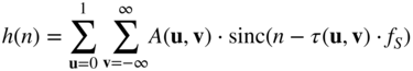
with
In Fig. 7.4, an exemplary room impulse response calculated via the image source model is shown. Here, the room dimensions are given as ![]() , and the receiver and source are positioned at
, and the receiver and source are positioned at ![]() and
and ![]() , respectively. Additionally, the absorption coefficient is set to
, respectively. Additionally, the absorption coefficient is set to ![]() for all walls. In Fig. 7.4 (top), the room impulse response is plotted for a length of
for all walls. In Fig. 7.4 (top), the room impulse response is plotted for a length of ![]() . Contrarily, Fig. 7.4 (bottom) focuses on the direct path and the first reflections, which illustrate also the sinc‐like characteristic of the individual reflections.
. Contrarily, Fig. 7.4 (bottom) focuses on the direct path and the first reflections, which illustrate also the sinc‐like characteristic of the individual reflections.

Figure 7.4 Simulated room impulse response via image source model with a length of  (top) and cutout of the direct path and the first reflections (bottom). The parameters are given as
  ,
,  ,
,  , and
, and  for all walls.
Finally, the order ![]() of a reflected path can be determined by
of a reflected path can be determined by
Although the image source model is able to calculate reflections up to an arbitrary order, practically, only low‐order reflections are calculated because of the strong increase of the number of image sources with rising order of reflections [Väl12].
7.1.3 Measurement of Room Impulse Responses
The direct measurement of a room impulse response is carried out by impulse excitation. Better measurement results are obtained by correlation measurement of the room impulse responses by using pseudo‐random sequences as the excitation signal. Pseudo‐random sequences can be generated by feedback shift registers [Mac76]. The pseudo‐random sequence is periodic with period ![]() , where
, where ![]() is the number of states of the shift register. The autocorrelation function (ACF) of such a random sequence is given by
is the number of states of the shift register. The autocorrelation function (ACF) of such a random sequence is given by

where ![]() is the maximum value of the pseudo‐random sequence. The ACF also has a period
is the maximum value of the pseudo‐random sequence. The ACF also has a period ![]() . After going through a DA converter, the pseudo‐random signal is fed through a loudspeaker into a room (see Fig. 7.5).
. After going through a DA converter, the pseudo‐random signal is fed through a loudspeaker into a room (see Fig. 7.5).

Figure 7.5 Measurement of room impulse response with pseudo‐random signal  .
.
At the same time, the pseudo‐random signal and the room signal captured by a microphone are recorded on a personal computer. The impulse response is obtained with the cyclic cross‐correlation:
For the measurement of room impulse responses, it has to be considered that the periodic length of the pseudo‐random sequence must be longer than the length of the room impulse response. Otherwise, aliasing in the periodic cross‐correlation ![]() (see Fig. 7.6) occurs. To improve the SNR of the measurement, the average of several periods of the cross‐correlation is calculated.
(see Fig. 7.6) occurs. To improve the SNR of the measurement, the average of several periods of the cross‐correlation is calculated.

Figure 7.6 Periodic auto‐correlation of pseudo‐random sequence and periodic cross‐correlation.
In [Far00, Far07], Farina proposed to use exponential sine sweeps as the excitation signal for measuring impulse responses. In comparison with other signals, the use of exponential sine sweeps has two major advantages [Hol09, Mül01, Sta02]. First, owing to the exponential increase in frequency, more energy is present at low frequencies, resulting in a higher SNR at low frequencies, which is particularly desirable in audio applications. Second, nonlinearities of the system under test are separated from the linear impulse response by the exponential sine sweep method.
A continuous‐time exponential sine sweep is defined as

where ![]() is the duration of the sweep in seconds, and
is the duration of the sweep in seconds, and ![]() and
and ![]() define the instantaneous angular frequencies at the beginning (
define the instantaneous angular frequencies at the beginning (![]() ) and the end of the sweep (
) and the end of the sweep (![]() ), respectively. Figure 7.7 illustrates the first half‐second of an exponential sine sweep
), respectively. Figure 7.7 illustrates the first half‐second of an exponential sine sweep ![]() with
with ![]() ,
, ![]() , and
, and ![]() . The evaluation of the period across time clearly indicates the increase in the frequency of the sine wave.
. The evaluation of the period across time clearly indicates the increase in the frequency of the sine wave.
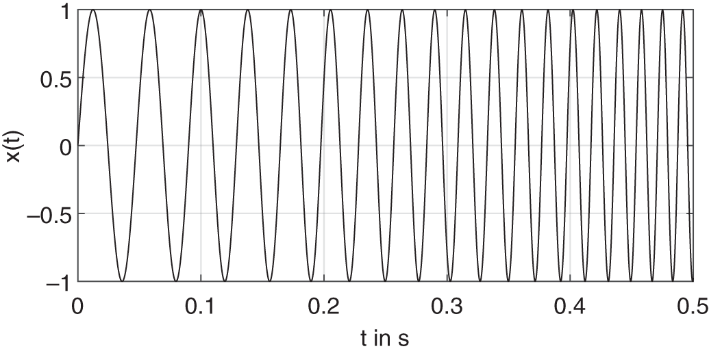
Figure 7.7 Beginning of an exponential sine sweep  with
with  ,
,  , and
, and  .
.
By calculating the derivative of the argument of the sine sweep ![]() with respect to time
with respect to time ![]() , the instantaneous angular frequency is determined as
, the instantaneous angular frequency is determined as

From this, the definition of the instantaneous angular frequencies at the beginning (![]() ) and the end (
) and the end (![]() ) of the sweep can be confirmed. Additionally, the exponential increase in frequency with time is explicitly shown. This increase is also visible in the spectrogram of the sine sweep shown in Fig. 7.8.
) of the sweep can be confirmed. Additionally, the exponential increase in frequency with time is explicitly shown. This increase is also visible in the spectrogram of the sine sweep shown in Fig. 7.8.

Figure 7.8 Spectrogram of an exponential sine sweep with  ,
,  , and
, and  .
.
For a digital implementation with a sampling rate of ![]() , the discrete‐time exponential sine sweep
, the discrete‐time exponential sine sweep

is used, where ![]() specifies the length of the sweep in samples, and
specifies the length of the sweep in samples, and ![]() and
and ![]() define the instantaneous normalized angular frequencies at the beginning (
define the instantaneous normalized angular frequencies at the beginning (![]() ) and the end (
) and the end (![]() ) of the sweep [Hol09]. Additionally, an inverse sine sweep
) of the sweep [Hol09]. Additionally, an inverse sine sweep ![]() can be defined as
can be defined as

where the first factor flips the sine sweep in time and the second factor is a correction factor that accounts for the equalization of the magnitude of the sine sweep. As can be seen in Fig. 7.9, the exponential increase of the frequency in the sine sweep ![]() results in a higher magnitude for low frequencies. Because a simple flipping of the sine sweep in time will not change the magnitude response, a correction factor is included to change the magnitude of the inverse sweep, as shown in Fig. 7.9.
results in a higher magnitude for low frequencies. Because a simple flipping of the sine sweep in time will not change the magnitude response, a correction factor is included to change the magnitude of the inverse sweep, as shown in Fig. 7.9.

Figure 7.9 Magnitude responses of the exponential sine sweep  , the inverse sine sweep
  , and the convolution result
  . Note that the magnitude responses are scaled by
  .
.
The convolution of the exponential sine sweep ![]() and the inverse sine sweep
and the inverse sine sweep ![]() results in a scaled and time‐shifted unit impulse
results in a scaled and time‐shifted unit impulse
where ![]() depends on the length of the inverse sweep and the correlation factor
depends on the length of the inverse sweep and the correlation factor ![]() is given in [Hol09] as
is given in [Hol09] as

Here, the approximation of the unit impulse ![]() results from the band limitation of the exponential sine sweep
results from the band limitation of the exponential sine sweep ![]() in the range of
in the range of ![]() to
to ![]() . Correcting the time shift and scaling using Eq. 7.25 yields the band‐limited unit impulse shown in Fig. 7.10. Furthermore, the magnitude response of the band‐limited unit impulse is shown in Fig. 7.9. In addition, the band limitation also overshoots and passband ripples can be seen in the magnitude responses, which can be reduced by applying fade in and fade out on the sine sweep in the time domain [Hol09].
. Correcting the time shift and scaling using Eq. 7.25 yields the band‐limited unit impulse shown in Fig. 7.10. Furthermore, the magnitude response of the band‐limited unit impulse is shown in Fig. 7.9. In addition, the band limitation also overshoots and passband ripples can be seen in the magnitude responses, which can be reduced by applying fade in and fade out on the sine sweep in the time domain [Hol09].

Figure 7.10 Result of the convolution of the exponential sine sweep  and the inverse sine sweep
  .
.
When using an exponential sine sweep as an excitation signal during impulse response measurements, the recorded signal ![]() is determined as
is determined as
where ![]() defines the impulse response of the system under test. Finally, the convolution of the recorded signal
defines the impulse response of the system under test. Finally, the convolution of the recorded signal ![]() and the inverse sine sweep
and the inverse sine sweep ![]() determines the measured impulse response
determines the measured impulse response ![]() as
as
with ![]() being the correlation factor defined in Eq. 7.26. Owing to the characteristics of the exponential sine sweep, this convolution separates the linear impulse response and the harmonic impulse responses of a nonlinear system in time [Hol09]. Here, a given frequency inside the
being the correlation factor defined in Eq. 7.26. Owing to the characteristics of the exponential sine sweep, this convolution separates the linear impulse response and the harmonic impulse responses of a nonlinear system in time [Hol09]. Here, a given frequency inside the ![]() th harmonic is reached
th harmonic is reached

samples before the excitation signal reaches this frequency. Thus, the ![]() th harmonic impulse response will be visible at
th harmonic impulse response will be visible at ![]() in the anti‐causal part of the measured impulse response. In Fig. 7.11, an exemplary measured room impulse response
in the anti‐causal part of the measured impulse response. In Fig. 7.11, an exemplary measured room impulse response ![]() is shown. Here, the parameters of the sweep are
is shown. Here, the parameters of the sweep are ![]() ,
, ![]() ,
, ![]() , and
, and ![]() . For a better representation, the maximum absolute amplitude of the impulse response is set to 1 and the linear impulse response is moved to
. For a better representation, the maximum absolute amplitude of the impulse response is set to 1 and the linear impulse response is moved to ![]() by reversing the time shift
by reversing the time shift ![]() introduced by the convolution. Furthermore, the impulse response is plotted in decibels rather than in linear scale. In addition to the linear impulse response at
introduced by the convolution. Furthermore, the impulse response is plotted in decibels rather than in linear scale. In addition to the linear impulse response at ![]() , the first and second harmonic impulse responses arise at
, the first and second harmonic impulse responses arise at ![]() and
and ![]() , respectively.
, respectively.

Figure 7.11 Exemplary measured room impulse response including the first and second harmonic impulse responses at  in the anti‐causal part. The sweep parameters are
  ,
,  ,
,  , and
, and  .
.
7.1.4 Simulation of Room Impulse Responses
The just described methods provide a means for calculating the impulse response out of the geometry of a room and for measuring the impulse response of a real room. The reproduction of such an impulse response is basically possible with the help of the fast convolution method, as described in Chapter 6. The ear signals at a listening position inside the room are computed by


where ![]() and
and ![]() are the measured impulse responses between the source inside the room, which generates the signal
are the measured impulse responses between the source inside the room, which generates the signal ![]() , and a dummy head with two ear microphones. Special implementations of fast convolution with low latency are described in [Soo90, Gar95, Rei95, Ege96, Joh00] and a hybrid approach based on convolution and recursive filters can be found in [Bro01]. Investigations regarding fast convolution with sparse psychoacoustic based room impulse responses are discussed in [Iid95, Lee03a, Lee03b].
, and a dummy head with two ear microphones. Special implementations of fast convolution with low latency are described in [Soo90, Gar95, Rei95, Ege96, Joh00] and a hybrid approach based on convolution and recursive filters can be found in [Bro01]. Investigations regarding fast convolution with sparse psychoacoustic based room impulse responses are discussed in [Iid95, Lee03a, Lee03b].
In Sections 7.2 and 7.3, we will consider special approaches for early reflections and subsequent reverberation, respectively, which allow a parametric adjustment of all relevant parameters of a room impulse response. With this approach, an accurate room impulse response is not possible, but with a moderate computational complexity, a satisfying solution from an acoustical point of view can be achieved, as shown in Section 7.4. In Section 7.5, an efficient implementation of the convolutions (7.30) and (7.31) with a multi‐rate signal processing approach [Zöl90, Sch92, Sch93, Sch94] will be discussed.
7.2 Early Reflections
Early reflections decisively affect room perception. Spatial impression is produced by early reflections which reach the listener laterally. The significance of lateral reflections in creating spatial impression was investigated by Barron [Bar71, Bar81]. Fundamental investigations of concert halls and their different acoustics have been described by Ando [And90].
7.2.1 Ando's Investigations
The results of the investigations by Ando are summarized in the following:
- Preferred delay time of a single reflection: with the ACF of the signal, the delay is determined by
 .
. - Preferred direction of a single reflection:
 .
. - Preferred amplitude of a single reflection:
 dB.
dB. - Preferred spectrum of a single reflection: no spectral shaping.
- Preferred delay time of a second reflection:
 .
. - Preferred reverberation time:
 .
.
These results show that in terms of perception, a preferred pattern of reflections as well as the reverberation time depend decisively on the audio signal. Hence, for different audio signals like classical music, pop music, speech, or musical instruments, entirely different requirements for early reflections and reverberation time have to be considered.
7.2.2 Gerzon Algorithm
The commonly used method of simulating early reflections is shown in Figs. 7.12 and 7.13. The signal is weighted and fed into a system generating early reflections, followed by an addition to the input signal. The first ![]() reflections are implemented by reading samples from a delay line and weighting these samples with a corresponding factor
reflections are implemented by reading samples from a delay line and weighting these samples with a corresponding factor ![]() (see Fig. 7.13). The design of a system for simulating early reflections will now be described, as proposed by Gerzon [Ger92].
(see Fig. 7.13). The design of a system for simulating early reflections will now be described, as proposed by Gerzon [Ger92].

Figure 7.12 Simulation of early reflections.
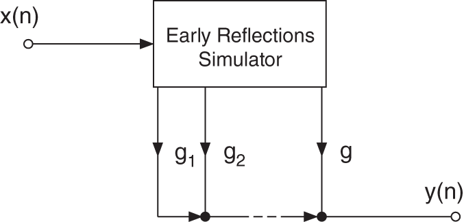
Figure 7.13 Early reflections.
Craven Hypothesis. The Craven hypothesis [Ger92] states that a human's perception of the distance to a sound source is evaluated with the help of the amplitude and delay time ratios of the direct signal and early reflections, as given by

with

Without a reflection, human beings are unable to determine the distance ![]() to a sound source. The extended Craven hypothesis includes the absorption coefficient
to a sound source. The extended Craven hypothesis includes the absorption coefficient ![]() for determining
for determining


For a given reverberation time ![]() , the absorption coefficient can be calculated by using
, the absorption coefficient can be calculated by using ![]() according to
according to
With the relationships (7.36) and (7.38), the parameters for an early reflections simulator, as shown in Fig. 7.12, can be determined.
Gerzon's Distance Algorithm. For a system simulating early reflections produced by more than one sound source, Gerzon's distance algorithm can be used [Ger92], where several sound sources are placed with different distances as well as in the stereo position into a stereophonic sound field. An application of this technique is mainly used in multichannel mixing consoles.
By shifting a sound source by ![]() (decrease of relative delay time), it follows that from the relative delay time of the first reflection
(decrease of relative delay time), it follows that from the relative delay time of the first reflection ![]() , and the relative amplitude according to (7.38),
, and the relative amplitude according to (7.38),

This results in a delay and a gain factor for the direct signal (see Fig. 7.14) as given by

Figure 7.14 Delay and weighting of the direct signal.
By shifting a sound source by ![]() (increase of relative delay time), the relative delay time of the first reflection is
(increase of relative delay time), the relative delay time of the first reflection is ![]() . As a consequence, a delay and a gain factor for the effect signal (see Fig. 7.15) are given by
. As a consequence, a delay and a gain factor for the effect signal (see Fig. 7.15) are given by
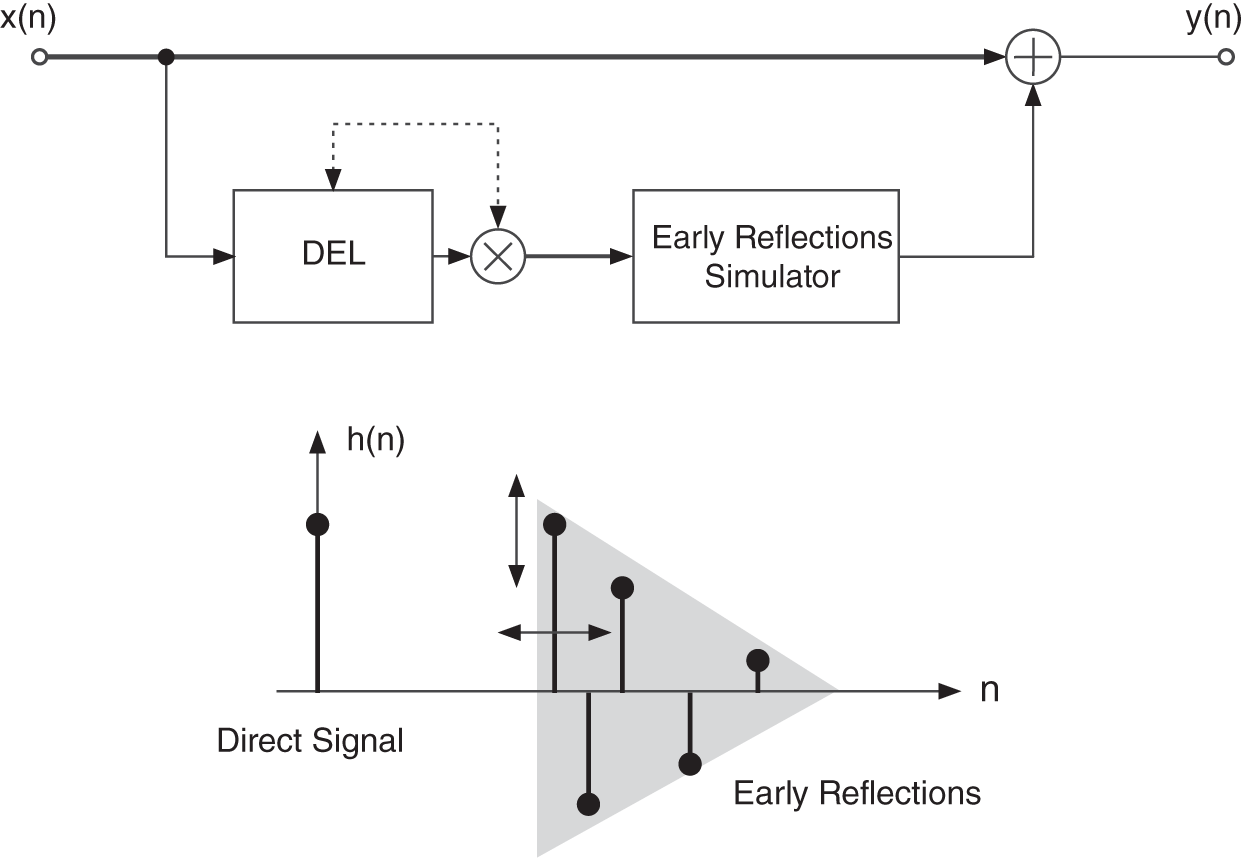
Figure 7.15 Delay and weighting of effect signal.

Figure 7.16 Coupled factors and delays.
Using two delay systems in the direct signal as well as in the reflection path, two coupled weighting factors and delay lengths (see Fig. 7.16) can be obtained. For multichannel applications like digital mixing consoles, the scheme in Fig. 7.17 is suggested by Gerzon [Ger92]. Only one system for implementing early reflections is necessary.

Figure 7.17 Multichannel application.
Stereo Implementation. In many applications, stereo signals have to be processed (see Fig. 7.18). For this, reflections from both sides with positive and negative angles are implemented to avoid stereo displacements. The weighting is done with

For each reflection, a weighting factor and an angle have to be considered.

Figure 7.18 Stereo reflections.
Generation of early reflection with increasing time density. In [Schr61], it is stated that the time density of reflections increases proportional to the square of time:
After time ![]() , the reflections have a statistical decay behavior. For a pulse width of
, the reflections have a statistical decay behavior. For a pulse width of ![]() , individual reflections overlap after
, individual reflections overlap after
To avoid an overlap of reflections, Gerzon [Ger92] suggests the increase of the density of reflections with ![]() (for example,
(for example, ![]() leads to
leads to ![]() or
or ![]() ). In the interval
). In the interval ![]() , with initial value
, with initial value ![]() and a number
and a number ![]() between 0.5 and 1, the following procedure is performed:
between 0.5 and 1, the following procedure is performed:
The numbers ![]() in the interval
in the interval ![]() are now transformed to time delays
are now transformed to time delays ![]() in the interval
in the interval ![]() by
by
The increase of the density of reflections is shown by the example in Fig. 7.19.

Figure 7.19 Increase of density for nine reflections.
7.3 Subsequent Reverberation
This section deals with techniques for reproducing subsequent reverberation. The first approaches by Schroeder [Schr61, Schr62] and their extension by Moorer [Moo78] will be described. Further developments by Stautner/Puckette [Sta82], Smith [Smi85], Dattarro [Dat97], and Gardner [Gar98] led to general feedback networks [Ger71, Ger76, Jot91, Jot92, Roc95, Roc97a, RS97b, Roc02], which have a random impulse response with exponential decay. An extensive discussion on the analysis and synthesis parameters of subsequent reverberation can be found in [Ble01]. An important parameter of subsequent reverberation [Cre03] is, in addition to the echo density, the quadratic increase of
with frequency. The following systems perform the quadratic increase in echo density and frequency density.
7.3.1 Schroeder Algorithm
The first software implementations of room simulation algorithms were carried out in 1961 by Schroeder. The basis for simulating an impulse response with exponential decay is a recursive comb filter, shown in Fig. 7.20.

Figure 7.20 Recursive comb filter ( feedback factor,
  delay length).
The transfer function is given by


with
With the correspondence of the Z‐transform ![]() , the impulse response is given by
, the impulse response is given by

The complex poles are combined as pairs so that the impulse response can be written as


The impulse response is expressed as a summation of cosine oscillations with frequencies ![]() . These frequencies correspond to the eigenfrequencies of a room. They decay with an exponential envelope
. These frequencies correspond to the eigenfrequencies of a room. They decay with an exponential envelope ![]() , where
, where ![]() is the damping constant (see Fig. 7.22a). The overall impulse response is weighted by
is the damping constant (see Fig. 7.22a). The overall impulse response is weighted by ![]() . The frequency response of the comb filter is shown in Fig. 7.22c and is given by
. The frequency response of the comb filter is shown in Fig. 7.22c and is given by

For positive ![]() , it shows maxima at
, it shows maxima at ![]() of magnitude
of magnitude

and minima at ![]() of magnitude
of magnitude

Another basis of the Schroeder algorithm is the allpass filter, shown in Fig. 7.21, with transfer function


From Eq. (7.67), it can be seen that the impulse response can also be expressed as a summation of cosine oscillations.

Figure 7.21 Allpass filter ( delay length).

Figure 7.22 (a) Impulse response of a comb filter ( = 10,
= 10,  = −0.6). (b) Impulse response of an allpass filter (
 = 10,
= 10,  = −0.6). (c) Frequency response of a comb filter. (d) Frequency response of an allpass filter.
The impulse responses and the frequency responses of a comb filter and an allpass filter are presented in Fig. 7.22 with a negative ![]() . Both impulse responses show an exponential decay. A sample in the impulse response occurs every
. Both impulse responses show an exponential decay. A sample in the impulse response occurs every ![]() sampling periods. The density of samples in the impulse responses does not increase with time. For the recursive comb filter, spectral shaping, owing to the maxima at the corresponding poles of the transfer function, is observed.
sampling periods. The density of samples in the impulse responses does not increase with time. For the recursive comb filter, spectral shaping, owing to the maxima at the corresponding poles of the transfer function, is observed.
Frequency Density
The frequency density describes the number of eigenfrequencies per Hertz and is defined for a comb filter [Jot91] as
A single comb filter gives ![]() resonances in the interval
resonances in the interval ![]() , which are separated by a frequency distance of
, which are separated by a frequency distance of ![]() . To increase the frequency density, a parallel circuit (see Fig. 7.23) of
. To increase the frequency density, a parallel circuit (see Fig. 7.23) of ![]() comb filters is used, which leads to
comb filters is used, which leads to

The choice of the delay systems [Schr62] is suggested as
and leads to a frequency density

In [Schr62], a necessary frequency density of ![]() eigenfrequencies per Hertz is proposed.
eigenfrequencies per Hertz is proposed.
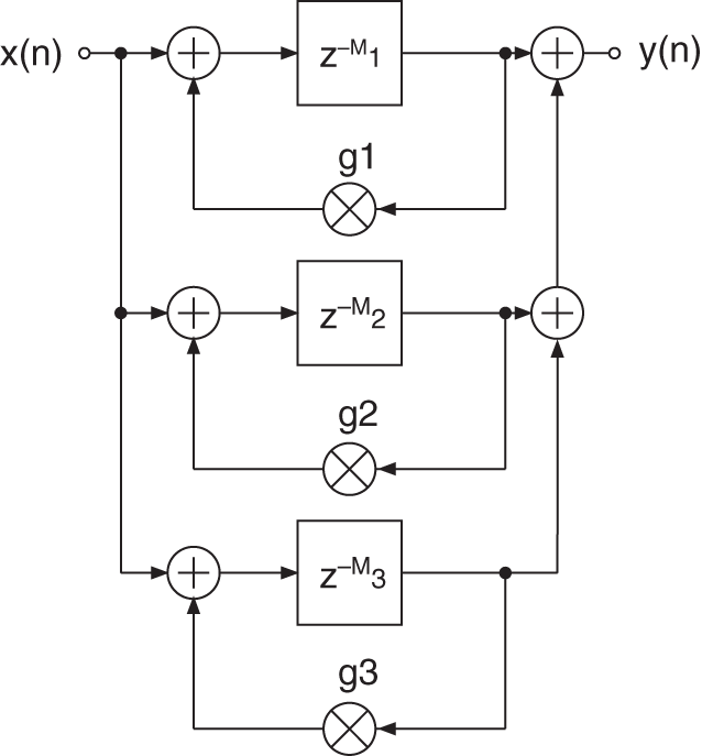
Figure 7.23 Parallel circuit of comb filters.
Echo Density
The echo density is the number of reflections per second and is defined for a comb filter [Jot91] as

For a parallel circuit of comb filters, the echo density is given by

With (Eqs. 7.71) and (7.73), the number ![]() of parallel comb filters and the mean delay length
of parallel comb filters and the mean delay length ![]() ,
,
are obtained. For a frequency density ![]() and an echo density
and an echo density ![]() , it can be concluded that the number of parallel comb filters is
, it can be concluded that the number of parallel comb filters is ![]() and the mean delay length is
and the mean delay length is ![]() ms. Because the frequency density is proportional to the reverberation time, the number of parallel comb filters has to be increased accordingly.
ms. Because the frequency density is proportional to the reverberation time, the number of parallel comb filters has to be increased accordingly.
A further increase of the echo density is achieved by a cascade circuit of ![]() allpass filters (see Fig. 7.24) with transfer function
allpass filters (see Fig. 7.24) with transfer function

These allpass sections are connected in series with the parallel circuit of comb filters. For a sufficient echo density, 10000 reflections per second are necessary [Gri89].

Figure 7.24 Cascade circuit of allpass filters.
Avoiding Unnatural Resonances
Because the impulse response of a single comb filter can be described as a sum of ![]() (delay length) decaying sinusoidal oscillations, the short‐time FFT of consecutive parts from this impulse response gives the frequency response shown in Fig. 7.25 in the time‐frequency domain. Only the maxima are presented. The parallel circuit of comb filters with the condition (7.70) leads to radii of the pole distribution, as given by
(delay length) decaying sinusoidal oscillations, the short‐time FFT of consecutive parts from this impulse response gives the frequency response shown in Fig. 7.25 in the time‐frequency domain. Only the maxima are presented. The parallel circuit of comb filters with the condition (7.70) leads to radii of the pole distribution, as given by ![]() . To avoid unnatural resonances, the radii of the pole distribution of a parallel circuit of comb filters must satisfy the condition:
. To avoid unnatural resonances, the radii of the pole distribution of a parallel circuit of comb filters must satisfy the condition:
This leads to the short‐time spectra and the pole distribution, as shown in Fig. 7.26. Figure 7.27 shows the impulse response and the echogram (logarithmic presentation of the amplitude of the impulse response) of a parallel circuit of comb filters with equal and unequal pole radii. For unequal pole radius, the different decay times of the eigenfrequencies can be seen.
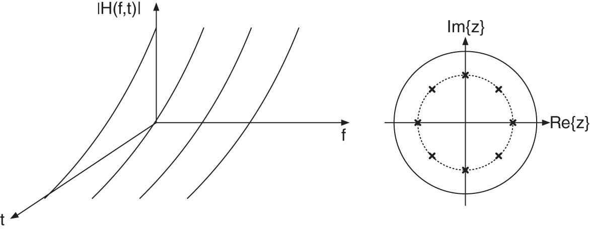
Figure 7.25 Short‐time spectra of a comb filter ( ).
).
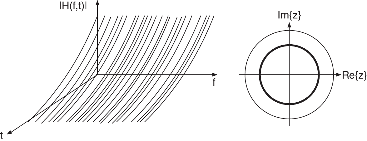
Figure 7.26 Short‐time spectra of a parallel circuit of comb filters.

Figure 7.27 Impulse response and echogram.
Reverberation Time
The reverberation time of a recursive comb filter can be adjusted with the feedback factor ![]() , which describes the ratio
, which describes the ratio

of two different non‐zero samples of the impulse response separated by ![]() sampling periods. The factor
sampling periods. The factor ![]() describes the decay constant per
describes the decay constant per ![]() samples. The decay constant per sampling period can be calculated from the pole radius
samples. The decay constant per sampling period can be calculated from the pole radius ![]() and is defined as
and is defined as

The relationship between feedback factor ![]() and pole radius
and pole radius ![]() can also be expressed using (Eqs. 7.78) and (7.79) and is given by
can also be expressed using (Eqs. 7.78) and (7.79) and is given by

With the constant radius ![]() and the logarithmic parameters
and the logarithmic parameters ![]() and
and ![]() , the attenuation per sampling period is given by
, the attenuation per sampling period is given by

The reverberation time is defined as the decay time of the impulse response to ![]() dB. With
dB. With ![]() , the reverberation time can be written as
, the reverberation time can be written as

The control of reverberation time can either be carried out with the feedback factor ![]() or the delay parameter
or the delay parameter ![]() . The increase of the reverberation time with factor
. The increase of the reverberation time with factor ![]() is responsible for a pole radius close to the unit circle and, hence, leads to an amplification of maxima of the frequency response (see Eq. (7.64)). This leads to a coloring of the sound impression. The increase of the delay parameter
is responsible for a pole radius close to the unit circle and, hence, leads to an amplification of maxima of the frequency response (see Eq. (7.64)). This leads to a coloring of the sound impression. The increase of the delay parameter ![]() , however, leads to an impulse response whose non‐zero samples are far apart from each other so that individual echoes can be heard. The discrepancy between echo density and frequency density for a given reverberation time can be solved by a sufficient number of parallel comb filters.
, however, leads to an impulse response whose non‐zero samples are far apart from each other so that individual echoes can be heard. The discrepancy between echo density and frequency density for a given reverberation time can be solved by a sufficient number of parallel comb filters.
Frequency‐dependent Reverberation Time
The eigenfrequencies of rooms have a rapid decay for high frequencies. A frequency‐dependent reverberation time can be implemented with a lowpass filter,
in the feedback loop of a comb filter. The modified comb filter in Fig. 7.28 has transfer function

with the stability criterion

Figure 7.28 Modified lowpass comb filter.
The short‐time spectra and the pole distribution of a parallel circuit with lowpass comb filters are presented in Fig. 7.29. Low eigenfrequencies decay slower than higher ones. The circular pole distribution becomes an elliptical distribution where the low‐frequency poles are moved toward the unit circle.

Figure 7.29 Short‐time spectra of a parallel circuit of lowpass comb filters.
Stereo Room Simulation
An extension of the Schroeder algorithm was suggested by Moorer [Moo78]. In addition to a parallel circuit of comb filters in series with a cascade of allpass filters, a pattern of early reflections is generated. Figure 7.30 shows a room simulation system for a stereo signal. The generated room signals ![]() and
and ![]() are added to the direct signals
are added to the direct signals ![]() and
and ![]() . The input of the room simulation is the mono signal
. The input of the room simulation is the mono signal ![]() (sum signal). This mono signal is added to the left and right room signals after going through a delay line DEL1. The total sum of all reflections is fed via another delay line DEL2 to a parallel circuit of comb filters which implements subsequent reverberation. To get a high‐quality spatial impression, it is necessary to decorrelate the room signals
(sum signal). This mono signal is added to the left and right room signals after going through a delay line DEL1. The total sum of all reflections is fed via another delay line DEL2 to a parallel circuit of comb filters which implements subsequent reverberation. To get a high‐quality spatial impression, it is necessary to decorrelate the room signals ![]() and
and ![]() [Bla74, Bla85]. This can be achieved by taking left and right room signals at different points out of the parallel circuit of comb filters. These room signals are then fed to an allpass section to increase the echo density.
[Bla74, Bla85]. This can be achieved by taking left and right room signals at different points out of the parallel circuit of comb filters. These room signals are then fed to an allpass section to increase the echo density.

Figure 7.30 Stereo room simulation.
In addition to the described system for stereo room simulation in which the mono signal is processed with a room algorithm, it is also possible to perform complete stereo processing of ![]() and
and ![]() , or to process a mono signal
, or to process a mono signal ![]() and a side (difference) signal
and a side (difference) signal ![]() individually.
individually.
7.3.2 General Feedback Systems
Further developments of the comb filter method by Schroeder tried to improve the acoustic quality of reverberation and especially the increase of echo density [Ger71, Ger76, Sta82, Jot91, Jot92, Roc95, Roc97a, RS97b]. With respect to [Jot91], the general feedback system in Fig. 7.31 is considered. For simplification, only three delay systems are shown. The feedback of output signals is carried out with the help of a matrix ![]() which feeds back each of the three outputs to the three inputs.
which feeds back each of the three outputs to the three inputs.

Figure 7.31 General feedback system.
In general, for ![]() delay systems, we can write
delay systems, we can write

The Z‐transform leads to

with
and the diagonal delay matrix
With Eq. (7.89), the Z‐transform of the output is given by
and the transfer function by
The system is stable if the feedback matrix ![]() can be expressed as a product of unitary matrix U (
can be expressed as a product of unitary matrix U (![]() ) and a diagonal matrix with
) and a diagonal matrix with ![]() (derivation in [Sta82]). Figure 7.32 shows a general feedback system with input vector
(derivation in [Sta82]). Figure 7.32 shows a general feedback system with input vector ![]() , the output vector
, the output vector ![]() , a diagonal matrix
, a diagonal matrix ![]() consisting of purely delay systems
consisting of purely delay systems ![]() , and a feedback matrix
, and a feedback matrix ![]() . This feedback matrix consists of an orthogonal matrix
. This feedback matrix consists of an orthogonal matrix ![]() multiplied by the matrix
multiplied by the matrix ![]() , which results in a weighting of the feedback matrix
, which results in a weighting of the feedback matrix ![]() .
.

Figure 7.32 Feedback system.
If an orthogonal matrix ![]() is chosen and the weighting matrix is equal to the unit matrix
is chosen and the weighting matrix is equal to the unit matrix ![]() , the system in Fig. 7.32 implements a white‐noise random signal with Gaussian distribution when a pulse excitation is applied to the input. The time density of this signal slowly increases with time. If the diagonal elements of the weighting matrix
, the system in Fig. 7.32 implements a white‐noise random signal with Gaussian distribution when a pulse excitation is applied to the input. The time density of this signal slowly increases with time. If the diagonal elements of the weighting matrix ![]() are less than one, a random signal with exponential amplitude decay results. With the help of the weighting matrix
are less than one, a random signal with exponential amplitude decay results. With the help of the weighting matrix ![]() , the reverberation time can be adjusted. Such a feedback system performs the convolution of an audio input signal with an impulse response of exponential decay.
, the reverberation time can be adjusted. Such a feedback system performs the convolution of an audio input signal with an impulse response of exponential decay.
The effect of the orthogonal matrix ![]() on the subjective sound perception of subsequent reverberation is of particular interest. A relationship between the distribution of the eigenvalues of the matrix
on the subjective sound perception of subsequent reverberation is of particular interest. A relationship between the distribution of the eigenvalues of the matrix ![]() on the unit circle and the poles of the system transfer function cannot be described analytically, owing to the high order of the feedback system. In [Her94], it is shown experimentally that the distribution of eigenvalues within the right‐hand or left‐hand complex plane produces a uniform distribution of poles of the system transfer function. Such a feedback matrix leads to an acoustically improved reverberation. The echo density rapidly increases to the maximum value of one sample per sampling period for a uniform distribution of eigenvalues. In addition to the feedback matrix, additional digital filtering is necessary to spectrally shape the subsequent reverberation and to implement frequency‐dependent decay times (see [Jot91]). The following example illustrates the increase of the echo density.
on the unit circle and the poles of the system transfer function cannot be described analytically, owing to the high order of the feedback system. In [Her94], it is shown experimentally that the distribution of eigenvalues within the right‐hand or left‐hand complex plane produces a uniform distribution of poles of the system transfer function. Such a feedback matrix leads to an acoustically improved reverberation. The echo density rapidly increases to the maximum value of one sample per sampling period for a uniform distribution of eigenvalues. In addition to the feedback matrix, additional digital filtering is necessary to spectrally shape the subsequent reverberation and to implement frequency‐dependent decay times (see [Jot91]). The following example illustrates the increase of the echo density.
7.3.3 Feedback Allpass Systems
In addition to the general feedback systems, simple delay systems with feedback have been used for room simulators (see Fig. 7.35). These simulators are based on a delay line, where single delays are fed back with ![]() feedback coefficients to the input. The sum of input signal and feedback signal is lowpass filtered or spectrally weighted by a low‐frequency shelving filter and is then put to the delay line again. The first
feedback coefficients to the input. The sum of input signal and feedback signal is lowpass filtered or spectrally weighted by a low‐frequency shelving filter and is then put to the delay line again. The first ![]() reflections are extracted out of the delay line according to the reflection pattern of the simulated room. They are weighted and added to the output signal. The mixing between the direct signal and the room signal is adjusted by the factor
reflections are extracted out of the delay line according to the reflection pattern of the simulated room. They are weighted and added to the output signal. The mixing between the direct signal and the room signal is adjusted by the factor ![]() . The inner system can be described by a rational transfer function
. The inner system can be described by a rational transfer function ![]() . To avoid a low frequency density, the feedback delay lengths can be made time variant [Gri89, Gri91].
. To avoid a low frequency density, the feedback delay lengths can be made time variant [Gri89, Gri91].

Figure 7.35 Room simulation with delay line and forward and backward coefficients.
Increasing the echo density can be achieved by replacing the delays ![]() by frequency‐dependent allpass systems
by frequency‐dependent allpass systems ![]() . This extension was first proposed by Gardner in [Gar92a, Gar92b, Gar92c, Gar98]. In addition to the replacement of
. This extension was first proposed by Gardner in [Gar92a, Gar92b, Gar92c, Gar98]. In addition to the replacement of ![]() , the allpass systems can be extended by embedded allpass systems [Gar92a, Gar92b, Gar92c]. Figure 7.36 shows an allpass system (Fig. 7.36a), where the delay
, the allpass systems can be extended by embedded allpass systems [Gar92a, Gar92b, Gar92c]. Figure 7.36 shows an allpass system (Fig. 7.36a), where the delay ![]() is replaced by a further allpass and a unit delay
is replaced by a further allpass and a unit delay ![]() (Fig. 7.36b). The integration of a unit delay avoids delay free loops. In Fig. 7.36c, the inner allpass is replaced by a cascade of two allpass systems and a further delay
(Fig. 7.36b). The integration of a unit delay avoids delay free loops. In Fig. 7.36c, the inner allpass is replaced by a cascade of two allpass systems and a further delay ![]() . The resulting system is again an allpass system [Gar92a, Gar92b, Gar92c, Gar98]. A further modification of the general allpass system is shown in Fig. 7.36d [Dat97, Vää97, Dah00]. Here, a delay
. The resulting system is again an allpass system [Gar92a, Gar92b, Gar92c, Gar98]. A further modification of the general allpass system is shown in Fig. 7.36d [Dat97, Vää97, Dah00]. Here, a delay ![]() followed by a lowpass and a weighting coefficient is used. The resulting system is called an absorbent allpass system. With these embedded allpass systems, the room simulator shown in Fig. 7.35 is extended to a feedback allpass system, which is shown in Fig. 7.37 [Gar92a, Gar92b, Gar92c, Gar98]. The feedback is performed by a lowpass filter and a feedback coefficient
followed by a lowpass and a weighting coefficient is used. The resulting system is called an absorbent allpass system. With these embedded allpass systems, the room simulator shown in Fig. 7.35 is extended to a feedback allpass system, which is shown in Fig. 7.37 [Gar92a, Gar92b, Gar92c, Gar98]. The feedback is performed by a lowpass filter and a feedback coefficient ![]() , which adjusts the decay behavior. The extension to a stereo room simulator is described in [Dat97, Dah00] and is depicted in Fig. 7.38 [Dah00]. The cascaded allpass systems
, which adjusts the decay behavior. The extension to a stereo room simulator is described in [Dat97, Dah00] and is depicted in Fig. 7.38 [Dah00]. The cascaded allpass systems ![]() in the left and right channel can be a combination of embedded and absorbent allpass systems. Both output signals of the allpass chains are fed back to the input and added. In front of both allpass chains, a coupling of both channels with a weighted sum and difference is performed. The setup and parameters of such a system are discussed in [Dah00]. A precise adjustment of reverberation time and control of echo density can be achieved by the feedback coefficients of the allpasses. The frequency density is controlled by the scaling of the delay lengths of the inner allpass systems.
in the left and right channel can be a combination of embedded and absorbent allpass systems. Both output signals of the allpass chains are fed back to the input and added. In front of both allpass chains, a coupling of both channels with a weighted sum and difference is performed. The setup and parameters of such a system are discussed in [Dah00]. A precise adjustment of reverberation time and control of echo density can be achieved by the feedback coefficients of the allpasses. The frequency density is controlled by the scaling of the delay lengths of the inner allpass systems.

Figure 7.36 Embedded and absorbing allpass system [Gar92a, Gar92b, Gar92c, Gar98, Dat97, Vää97, Dah00].

Figure 7.37 Room simulator with embedded allpass systems [Gar92a, Gar92b, Gar92c, Gar98].

Figure 7.38 Stereo room simulator with absorbent allpass systems. Modified from [Dah00].
The original Schroeder comb and allpass reverberator was further improved by moving the allpass filters into the parallel arrangement of ![]() allpass
allpass ![]() and delay
and delay ![]() sections [Spin]. The principle structure is shown in Fig. 7.39.
sections [Spin]. The principle structure is shown in Fig. 7.39.

Figure 7.39 Simplified feedback delay network containing parallel allpass/delay branches.
The feedback of each allpass/delay branch into the next parallel allpass/delay and feeding the last allpass/delay back to the first via a feedback coefficient ![]() leads to a simplified feedback delay network with a sparse feedback matrix. The input state variables to the allpasses are given by
leads to a simplified feedback delay network with a sparse feedback matrix. The input state variables to the allpasses are given by

and for the output of the allpasses according to
where ![]() and
and ![]() define the delay and the coefficient inside the
define the delay and the coefficient inside the ![]() allpass, respectively. It is effectively a loop of several allpass/delays with a decay coefficient and a possible additional HF shelving filter for simulating air damping. The input is fed into each parallel section and the output is a weighted sum of all parallel sections given by
allpass, respectively. It is effectively a loop of several allpass/delays with a decay coefficient and a possible additional HF shelving filter for simulating air damping. The input is fed into each parallel section and the output is a weighted sum of all parallel sections given by

For a stereo output, a second weighted sum with orthogonal coefficients can be applied. The feedback coefficient and the HF shelving filter adjust the reverberation time. The room size can be adjusted by scaling the delays inside the allpasses and delays accordingly.
7.4 Approximation of Room Impulse Responses
In contrast to the systems for simulation of room impulse responses discussed up to this point, a method is now presented that measures and approximates the room impulse response in one step [Zöl90, Sch92, Sch93] (see Fig. 7.40). Moreover, it leads to a parametric representation of the room impulse response. Because the decay times of room impulse responses decrease for high frequencies, use is made of multirate signal processing.

Figure 7.40 System measuring and approximating room impulse responses.
The analog system that is to be measured and approximated is excited with a binary pseudo‐random sequence ![]() via a DA converter. The resulting room signal gives a digital sequence
via a DA converter. The resulting room signal gives a digital sequence ![]() after AD conversion. The discrete‐time sequence
after AD conversion. The discrete‐time sequence ![]() and the pseudo‐random sequence
and the pseudo‐random sequence ![]() are each decomposed by an analysis filter bank into sub‐band signals
are each decomposed by an analysis filter bank into sub‐band signals ![]() and
and ![]() , respectively. The sampling rate is reduced in accordance with the bandwidth of the signals. The sub‐band signals
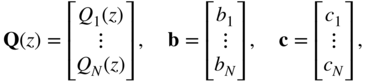
, respectively. The sampling rate is reduced in accordance with the bandwidth of the signals. The sub‐band signals ![]() are approximated by adjusting the sub‐band systems
are approximated by adjusting the sub‐band systems ![]() . The outputs
. The outputs ![]() of these sub‐band systems give an approximation of the measured sub‐band signals. With this procedure, the impulse response is given in parametric form (sub‐band parameters) and can be directly simulated in the digital domain.
of these sub‐band systems give an approximation of the measured sub‐band signals. With this procedure, the impulse response is given in parametric form (sub‐band parameters) and can be directly simulated in the digital domain.
By suitably adjusting the analysis filter bank [Sch94], the sub‐band impulse responses are obtained directly from the cross‐correlation function
The sub‐band impulse responses are approximated by a non‐recursive filter and a recursive comb filter. The cascade of both filters leads to the transfer function
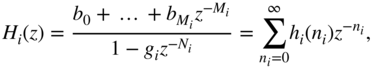
which is set equal to the impulse response in sub‐band ![]() . Multiplying both sides of Eq. (7.100) by the denominator
. Multiplying both sides of Eq. (7.100) by the denominator ![]() gives
gives

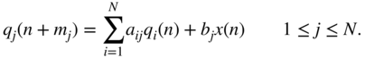
Truncating the impulse response of each sub‐band to ![]() samples and comparing the coefficients of powers of
samples and comparing the coefficients of powers of ![]() on both sides of the equation, the following set of equations is obtained:
on both sides of the equation, the following set of equations is obtained:

The coefficients ![]() and
and ![]() in the above equation are determined in two steps. First, the coefficient
in the above equation are determined in two steps. First, the coefficient ![]() of the comb filter is calculated from the exponentially decaying envelope of the measured sub‐band impulse response. The vector
of the comb filter is calculated from the exponentially decaying envelope of the measured sub‐band impulse response. The vector ![]() is then used to determine the coefficients
is then used to determine the coefficients ![]() .
.
For the calculation of the coefficient ![]() , we start with the impulse response of the comb filter
, we start with the impulse response of the comb filter ![]() given by
given by
We further make use of the integrated impulse response

defined in [Schr65]. It describes the rest energy of the impulse response at time ![]() . By taking the logarithm of
. By taking the logarithm of ![]() , a straight line over time index
, a straight line over time index ![]() is obtained. From the slope of the straight line, we use
is obtained. From the slope of the straight line, we use

to determine the coefficient ![]() [Sch94]. For
[Sch94]. For ![]() , the coefficients in Eq. (7.102) of the numerator polynomial are obtained directly from the impulse response
, the coefficients in Eq. (7.102) of the numerator polynomial are obtained directly from the impulse response

Hence, the numerator polynomial of Eq. (7.100) is a direct reproduction of the first ![]() samples of the impulse response (see Fig. 7.41). The denominator polynomial approximates the further exponentially decaying impulse response. This method is applied to each sub‐band. The implementation complexity can be reduced by a factor of 10 compared with the direct implementation of the broadband impulse response [Sch94]. However, owing to the group delay caused by the filter bank, this method is not suitable for real‐time applications.
samples of the impulse response (see Fig. 7.41). The denominator polynomial approximates the further exponentially decaying impulse response. This method is applied to each sub‐band. The implementation complexity can be reduced by a factor of 10 compared with the direct implementation of the broadband impulse response [Sch94]. However, owing to the group delay caused by the filter bank, this method is not suitable for real‐time applications.

Figure 7.41 Determining model parameters from the measured impulse response.
7.5 JS Applet – Fast Convolution
The applet shown in Fig. 7.42 demonstrates audio effects resulting from a fast convolution algorithm. It is designed for a first insight into the perceptual effects of convolving an impulse response with an audio signal.
The applet generates an impulse response by modulating the amplitude of a random signal. The graphical interface presents the curve of the amplitude modulation, which can be manipulated with three control points. Two control points are used for the initial behavior of the amplitude modulation. The third control point is used for the exponential decay of the impulse response. You can choose between two predefined audio files from our web server (audio1.wav or audio2.wav) or your own local WAV file to be processed [Gui05].

Figure 7.42 JS applet – fast convolution.
7.6 Exercises
1. Room Impulse Responses
- How can we measure a room impulse response?
- What kind of test signal is necessary?
- How does the length of the impulse response affect the length of the test signal?
2. First Reflections
For a given sound (voice sound), calculate the delay time of a single first reflection. Write a Matlab program for the following computations.
- Why do we have to choose this delay time? What coefficient should be used for this delay time?
- Write an algorithm which performs the convolution of the input mono signal with two impulse responses which simulate a reflection to the left output
 and a second reflection to the right output
  . Check the results by listening to the output sound.
 - Improve your algorithm to simulate two reflections which can be positioned to any angle inside the stereo mix.
3. Comb and Allpass Filters
- Comb Filters: Based on the Schroeder algorithm, draw a signal flow graph for a comb filter consisting of a single delay line of
 samples with a feedback loop containing an attenuation factor
  .
.
- Derive the transfer function of the comb filter.
- Now, the attenuation factor
 is in the feed‐forward path and in the feedback loop no attenuation is applied. Why can we consider the impulse response of this model to be similar to the previous one?
 - In both cases, how should we choose the gain factor? What will happen if we do not respect that?
- Calculate the reverberation time of the comb filter for
 kHz,
kHz,  =8, and
  specified previously.
 - Make a statement about the filter coefficients, and plot the pole/zero locations and the frequency response of the filter.
- Allpass Filters: Realize an allpass structure as suggested by Schroeder.
- Why can we expect a better result with an allpass filter than with a comb filter? Write a Matlab function for a comb and allpass filter with
 .
. - Derive the transfer function and show the pole/zero locations, and the impulse, the magnitude, and phase responses.
- Perform the filtering of an audio signal with the two filters and estimate the delay length
 , which leads to a perception of a room impression.
- Why can we expect a better result with an allpass filter than with a comb filter? Write a Matlab function for a comb and allpass filter with
4. Feedback Delay Networks
Write a Matlab program which realizes an FDN system.
- What is the reason for a unitary feedback matrix?
- What is the advantage of using a unitary circulant feedback matrix?
- How do you control the reverberation time?
References
- [Ant02] J. Antonio, L. Godinho, and A. Tadeu:Reverberation times obtained using a numerical model versus those given by simplified formulas and measurements. Acta Acustica, 88:25–261, 2002.
- [All79] J.B. Allen, D.A. Berkeley: Image Method for Efficient Simulating Small Room Acoustics, J. Acoust. Soc. Am., Vol. 65, No. 4, pp. 943–950, 1979.
- [And90] Y. Ando: Concert Hall Acoustics, Springer‐Verlag, 1990.
- [Bro01] S. Browne: Hybrid Reverberation Algorithm Using Truncated Impulse Response Convolution and Recursive Filtering, MSc Thesis, University of Miami, Coral Gables, Florida, June, 2001.
- [Bar71] M. Barron: The Subjective Effects of First Reflections in Concert Halls ‐ The Need for Lateral Reflections, J. Sound and Vibration 15, pp. 475–494, 1971.
- [Bar81] M. Barron, A.H. Marschall: Spatial Impression Due to Early Lateral Reflections in Concert Halls: The Derivation of a Physical Measure, J. Sound and Vibration 77, pp. 211–232, 1981.
- [Bel99] F.A. Beltran, J.R. Beltran, N. Holzem, and A. Gogu: Matlab Implementation of Reverberation Algorithms, Proc. Workshop on Digital Audio Effects (DAFx‐99), pp. 91–96, Trondheim, Norway, 1999.
- [Bla74] J. Blauert: Räumliches Hören, S. Hirzel Verlag, Stuttgart, 1974.
- [Bla85] J. Blauert: Räumliches Hören, Nachschrift‐Neue Ergebnisse und Trends seit 1972, S. Hirzel Verlag, Stuttgart, 1985.
- [Ble01] B. Blesser: An Interdisciplinary Synthesis of Reverberation Viewpoints, J. Audio Eng. Soc., 49(10):867–903, October 2001.
- [Cre78] L. Cremer, H.A. Müller: Die wissenschaftlichen Grundlagen der Raumakustik ‐ Bd. 1 u. 2, S. Hirzel Verlag, Stuttgart, 1978/76.
- [Cre03] L. Cremer, M. Möser: Technische Akustik, Springer‐Verlag, Berlin, 2003.
- [Dah00] L. Dahl, J.‐M. Jot: A Reverberator based on Absorbent All‐pass Filters, in Proceedings of the COST G‐6 Conference on Digital Audio Effects (DAFX‐00), Verona, Italy, December 7‐9, 2000.
- [Dat97] J. Dattorro: Effect design ‐ Part 1: Reverberator and other Filters, J. Audio Eng. Soc., 45(19):660–684, September 1997.
- [Ege96] G. P. M. Egelmeers and P. C. W. Sommen: A new method for efficient convolution in frequency domain by nonuniform partitioning for adaptive filtering, IEEE Trans. Signal Processing, Vol. 44, pp. 3123–3192, Dec. 1996.
- [Far00] A. Farina: Simultaneous Measurement of Impulse Response and Distortion with a Swept‐sine Technique, Proc. 108th AES Convention, Paris 18‐22, February 2000.
- [Far07] A. Farina: Advancements in impulse response measurements by sine sweeps. In Audio Engineering Society Convention 122, May 2007.
- [Fre00] J. Frenette: Reducing Artificial Reverberation Algorithm Requirements Using Time‐varying Feddback Delay Networks, MSc Thesis, University of Miami, Coral Gables, Florida, December 2000.
- [Gar92a] W.G. Gardner: A Realtime Multichannel Room Simulator, J. Acoust. Soc. Am., Vol. 92 (4(A)):2395, 1992.
- [Gar92b] W.G. Gardner: Reverb ‐ A Reverberator Design Tool for Audiomedia, Proc. Int. Comp. Music Conf. (San Jose, CA), 1992.
- [Gar92c] W.G. Gardner: The Virtual Acoustic Room, Master's Thesis, MIT Media Lab, 1992.
- [Gar95] W. G. Gardner: Efficient Convolution Without Input‐output Delay, J. Audio Eng. Soc., 43(3), pp. 127–136,1995.
- [Gar98] W.G. Gardner: Reverberation Algorithms, In M. Kahrs and K. Brandenburg (eds), Applications of Digital Signal Processing to Audio and Acoustics, Kluwer Academic Publishers, p. 85–131, 1998.
- [Ger71] M.A. Gerzon: Synthetic Stereo Reverberation, Studio Sound, no. 13, pp. 632–635, 1971 und no. 14, pp. 24–28, 1972.
- [Ger76] M.A. Gerzon: Unitary (Energy‐Preserving) Multichannel Networks with Feedback, Electronics Letters, Vol. 12, No. 11, pp. 278–279, 1976.
- [Ger92] M.A. Gerzon: The Design of Distance Panpots, Proc. 92nd AES Convention, Preprint No. 3308, Vienna, 1992.
- [Gri89] D. Griesinger: Practical Processors and Programs for Digital Reverberation, Proc. AES 7th Int. Conf., pp. 187–195, Toronto, 1989.
- [Gri91] D. Griesinger: Improving Room Acoustics Through Time‐Variant Synthetic Reverberation, in Proc. 90th Conv. Audio Eng. Soc., Preprint 3014, Feb. 1991.
- [Gui05] M. Guillemard, C. Ruwwe, U. Zölzer: J‐DAFx ‐ Digital Audio Effects in Java, Proc. 8th Int. Conference on Digital Audio Effects (DAFx‐05), Madrid, Spain, pp.161–166, 2005.
- [Her94] T. Hertz: Implementierung und Untersuchung von Rückkopplungssystemen zur digitalen Raumsimulation, Diplomarbeit, TU Hamburg‐Harburg, 1994.
- [Hol09] M. Holters, T. Corbach, and U. Zölzer: Impulse response measurement techniques and their applicability in the real world. In Proc. of the 12th Int. Conference on Digital Audio Effects (DAFx‐09), Como, Italy, September 1st‐4th 2009.
- [Iid95] K. Iida, K. Mizushima, Y. Takagi, and T. Suguta: A New Method of Generating Artificial Reverberant Sound, Proc. 99th AES Convention 1995, Preprint No. 4109, October 6‐9, 1995.
- [Joh00] M. Joho, G.S. Moschytz: Connecting Partitioned Frequency‐Domain Filters in Parallel or in Cascade, IEEE Trans. CAS‐II: Analog and Digital Signal Processing, Vol. 47, No. 8, pp. 685–698, Aug. 2000.
- [Jot91] J.M. Jot, A. Chaigne: Digital Delay Networks for Designing Artificial Reverberators, Proc. 94th AES Convention, Preprint No. 3030, 1991.
- [Jot92] J.M. Jot: An Analysis/Synthesis Approach to Real‐Time Artificial Reverberation, Proc. ICASSP‐92, pp. 221–224, San Francisco, 1992.
- [Ken95a] G.S. Kendall: A 3‐D sound primer: directional hearing and stereo reproduction, Computer Music J., 19(4):23–46, Winter 1995.
- [Ken95b] G.S. Kendall. The decorrelation of audio signals and its impact on spatial imagery, Computer Music J., 19(4):71–87, Winter 1995.
- [Kut91] H. Kuttruff: Room Acoustics, 3rd Edition, Elsevier Applied Sciences, London, 1991.
- [Lee03a] W.‐C. Lee, C.‐M. Liu, C.‐H. Yang, and J.‐I. Guo, Perceptual Convolution for Reverberation, Proc. 115th Convention 2003, Preprint No. 5992, October 10‐13, 2003
- [Lee03b] W.‐C. Lee, C.‐M. Liu, C.‐H. Yang, and J.‐I. Guo, Fast Perceptual Convolution for Reverberation, In Proc. of the 6th Int. Conference on Digital Audio Effects (DAFX‐03), London, UK, September 8‐11, 2003.
- [Leh08] E.A. Lehmann and A.M. Johansson: Prediction of energy decay in room impulse responses simulated with an image‐source model. The Journal of the Acoustical Society of America, 124(1):269–277, June 2008.
- [Lok01] T. Lokki, J. Hiipakka: A Time‐variant Reverberation Algorithm for Reverberation Enhancement Systems In Proc. of the COST G‐6 Conference on Digital Audio Effects (DAFX‐01), Limerick, Ireland, December 6‐8, 2001.
- [Moo78] J.A. Moorer: About this Reverberation Business, Computer Music Journal, Vol. 3, No. 2, pp. 13–28, 1978.
- [Mac76] F.J. MacWilliams, N.J.A. Sloane: Pseudo‐Random Sequences and Arrays, IEEE Proceedings, Vol. 64, pp. 1715–1729, 1976.
- [Mül01] S. Müller, P. Massarani: Transfer‐Function Measurement with Sweeps, J. Audio Eng. Soc., Vol. 49, pp. 443–471, 2001.
- [Pii98] E. Piirilä, T. Lokki, V. Välimäki, Digital Signal Processing Techniques for Non‐exponentially Decaying Reverberation, in Proc. 1st COST‐G6 Workshop on Digital Audio Effects (DAFX98) (Barcelona, Spain), 1998.
- [Soo90] J.S. Soo, K.K. Pang: Multidelay Block Frequency Domain Adaptive Filter, IEEE Trans. ASSP, Vol. 38, No. 2, pp. 373–376, Feb. 1990.
- [Rei95] A.J. Reijen, J.J. Sonke, and D. de Vries: New Developments in Electro‐Acoustic Reverberation Technology, Proc. 98th AES Convention 1995, Preprint No. 3978, February 25‐28, 1995.
- [Roc95] D. Rocchesso: The Ball within the Box: a sound‐processing metaphor, Computer Music J., 19(4):47–57, Winter 1995.
- [Roc97a] D. Rocchesso: Maximally‐diffusive yet efficient feedback delay networks for artifcial reverberation, IEEE Signal Processing Letters, 4(9):252–255, September 1997.
- [RS97b] D. Rocchesso and J.O. Smith: Circulant and elliptic feedback delay net‐ works for artificial reverberation, IEEE Transactions on Speech and Audio Processing, 5(1):51–63, January 1997.
- [Roc02] D. Rocchesso: Spatial Effects, In U. Zölzer (eds), DAFX ‐Digital Audio Effects, J. Wiley & Sons, p. 137–200, 2002.
- [Sch92] M. Schönle, U. Zölzer, N. Fliege: Modeling of Room Impulse Responses by Multirate Systems, Proc. 93rd AES Convention, Preprint No. 3447, San Francisco 1992.
- [Sch93] M. Schönle, N.J. Fliege, U. Zölzer: Parametric Approximation of Room Impulse Responses by Multirate Systems, Proc. ICASSP‐93, Vol. 1, pp. 153–156, 1993.
- [Sch94] M. Schönle: Wavelet‐Analyse und parametrische Approximation von Raumimpulsantworten, Dissertation, TU Hamburg‐Harburg, 1994.
- [Schr61] M.R. Schroeder, B.F. Logan: Colorless Artificial Reverberation, J. Audio Eng. Soc., Vol. 9(3), pp. 192–197, 1961.
- [Schr62] M.R. Schroeder: Natural Sounding Artificial Reverberation, J. Audio Eng. Soc., Vol. 10(3), pp. 219–223, 1962.
- [Schr65] M.R. Schroeder: New Method of Measuring Reverberation Time, J. Acoust. Soc. Am., pp. 409–412, 1965.
- [Schr70] M.R. Schroeder: Digital Simulation of Sound Transmission in Reverberant Spaces, J. Acoust. Soc. Am., Vol. 47, No. 2, pp. 424–431, 1970.
- [Schr87] M.R. Schroeder: Statistical Parameters of the Frequency Response Curves of Large Rooms, J. Audio Eng. Soc., Vol. 35, No. 5, pp. 299–305, 1987.
- [Smi85] J.O. Smith: A new approach to digital reverberation using closed waveguide networks, In Proc. International Computer Music Conference, pp. 47–53, Vancouver, Canada, 1985.
- [Spin]Spin Semiconductor: Audio effects. http://www.spinsemi.com, accessed: 2021‐05‐20.
- [Sta02] G.B. Stan, J.J. Embrechts, D. Archambeau: Comparison of Different Impulse Response Measurement Techniques, J. Audio Eng. Soc., Vol. 50, pp. 249–262, 2002.
- [Sta82] J. Stautner, M. Puckette: Designing Multi‐Channel Reverberators, Computer Music Journal, Vol. 6, No. 1, pp. 56–65, 1982.
- [Vää97] R. Väänänen, V. Välimäki, and J. Huopaniemi: Efficient and Parametric Reverberator for Room Acoustics Modeling, in Proc. Int. Computer Music Conf. (ICMC'97), pp. 200–203, Thessaloniki, Greece, Sept. 1997.
- [Väl12] V. Välimäki, J. D. Parker, L. Savioja, J. O. Smith, and J. S. Abel: Fifty years of artificial reverberation. IEEE Transactions on Audio, Speech, and Language Processing, 20(5):1421–1448, 2012.
- [Zöl90] U. Zölzer, N.J. Fliege, M. Schönle, M. Schusdziarra: Multirate Digital Reverberation System, Proc. 89th AES Convention, Preprint No. 2968, Los Angeles 1990.