CHAPTER 7

Introduction to Extend

This chapter introduces the simulation software called Extend¹. This tool will be applied to the analysis and design of business processes. The general Extend package is not industry specific, so it can be used to model and simulate discrete-event or continuous systems in a wide variety of settings ranging from production processes to population-growth models. The BPR library within this software was created for the specific purpose of modeling and simulating business processes. This special functionality of Extend is utilized throughout Chapters 7, 8, 9, and 10.

The best way to learn the material discussed in this chapter is in front of a computer. Students should install Extend and open the application to either create the models shown in this chapter or review the models that are distributed in the CD that accompanies this book. For convenience, all the models used for illustration purposes have been included in the CD. The models are named Figurexx.xx.mox; xx.xx is the number that corresponds to the figure number in the book. For instance, the first model that is discussed in this chapter is the one that appears in Figure 7.2, so the corresponding file is Figure07.02.mox.

The development of a simulation model using Extend entails the following steps.

1. Determine the goals of the model.
2. Understand the process to be modeled through the use of basic analysis and design tools, such as flowcharting.
3. Draw a block diagram using the appropriate blocks in the available libraries to represent each element of the model accurately.
4. Specify appropriate parameter values for each block.
5. Define the logic of the model and the appropriate connections between blocks.
6. Validate the model.
7. Add data collection and graphical analysis capabilities.
8. Analyze the output data and draw conclusions.

Before building a model, the analyst must think about what questions the model is supposed to answer. For example, if the goal is to examine the staffing needs of a process, many details that are not related to process capacity can be left out of the model. The level of detail and the scope of the model are directly related to the overall goal of the simulation effort. Because the model will help the analyst predict process performance, a good starting point is to define what constitutes “good” performance. This definition can be used later to enhance the process design via optimization².

Before modeling processes within the simulator’s environment, the analyst needs to understand the process thoroughly. This implies that the analyst knows the activities in the process, the sequence in which they are performed, the resources needed to perform the activities, and the logical relationships among activities. This understanding includes the knowledge of the arrival and service process for each activity. In particular, the analyst must be able to estimate the probability distributions that govern the behavior of arrivals to the process and the time needed to complete each activity. This step usually requires some statistical analysis to determine appropriate probability distributions associated with the processing times in each activity and the time between job arrivals. Typically, data are collected for the processing times in each activity and then a distribution is fitted to the data. Similarly, data are collected to figure out what distribution best represents the arrival pattern. A statistical test, such as the Chi-square, can be used for this purpose, as discussed in Chapter 9. ExpertFit (www.averill-law.com) and Stat::Fit (www.geerms.com) are two software packages that can be used to determine automatically and accurately what probability distribution best represents a set of real-world data. These products are designed to fit continuous and discrete distributions and to provide relative comparisons among distribution types. The use of Stat::Fit is illustrated in Chapter 9.

Extend, like most modern simulation packages, provides a graphical modeling environment. This environment consists of representing the actual process as a block diagram. Modeling in Extend entails the appropriate selection of blocks and their interconnection. Blocks are used to model activities, resources, and the routing of jobs throughout the process. Additional blocks are used to collect data, calculate statistics, and display output graphically with frequency charts, histograms, and line plots. Extend also includes blocks to incorporate activity-based costs in the simulation model, as explained in Chapter 8.

The most basic block diagram of a business process starts with the representation of the activities in the process. Then the conditions that determine the routing of jobs through the process, and if appropriate, a representation of resources, is included. In addition, rules are provided to define the operation of queues and the use of available resources. Finally, data collection and displays of summarized output data are added to the model.

In order to measure performance, the analyst must determine whether additional blocks are needed. If performance is measured by the waiting time in the queues, no additional blocks are necessary because the blocks that model queues collect waiting time data. The same goes for resource blocks and utilization data. However, if the analyst wants to count the number of jobs that are routed through a particular activity during a given simulation, a Count Items block (from the Information submenu of the Discrete Event library) needs to be included in the model. Extend libraries also include blocks that can be used to collect other important data, such as cycle times.

One of the most important aspects of a simulation is the definition and monitoring of resources. As discussed in Chapter 5, resources are needed to perform activities, and resource availability determines process capacity. Therefore, for a simulation model of a business process to be useful, resources must be defined and the resource requirements for each activity must be specified. Extend provides a Labor Pool, in the Resources submenu of the BPR library, that is used to define the attributes of each resource type, including availability and usage. A Labor Pool may represent, for instance, a group of nurses in a hospital. Every time a nurse starts or finishes performing an activity, the number of available nurses is adjusted in the Labor Pool block. These blocks are particularly useful for determining staffing needs based on performance measures such as queue length, waiting time, and resource utilization.

The proper completion of these steps results in a simulation model that describes the actual process (at a level of detail that is consistent with the goals outlined in step 1). Because in all likelihood some mathematical and logical expressions will be used during the modeling effort, it is necessary to check that the syntax employed to write these expressions is indeed correct. Checking the syntax allows the analyst to create a simulation model that is operational. A computer simulation cannot be executed until the syntax is completely correct.

Not all simulation models that run are valid; that is, one can develop a simulation model where jobs arrive, flow through the process, and leave. However, this does not mean that the model represents the actual process accurately. Model validation is an essential step in building simulations. The validation of a model consists of ensuring that the operational rules and logic in the model are an accurate reflection of the real system. Model validation must occur before the simulation results are used to draw conclusions about the behavior of the process.

7.1 Extend Elements

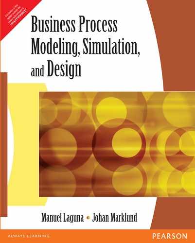
A simulation model in Extend is an interconnected set of blocks. A block performs a specific function, such as simulating an activity, a queue, or a pool of resources. A library is a repository of blocks. In order to use a particular block in a model, the library in which the block resides must be open. The tutorial of Section 7.2 will show how to open libraries. A simple simulation model of a process can be constructed using five basic blocks. (See Figure 7.1.)

• The Executive block from the Discrete Event library is a special block that must be included in all business process simulations. The block controls the timing and passing of events in the model. This block is the heart of a business process simulation and must be placed to the left of all other blocks in the block diagram. (JYpically, the Executive block is placed at the upper-left comer of the simulation model.)
• The Import block from the Generators submenu of the BPR library is used to generate items at arrival times specified in the dialogue box. When developing the model, one must determine what items will be generated, for example jobs, customers, purchasing orders, insurance claims, or patients, to name a few.
• The Repository block from the Resources submenu of the BPR library is similar to a holding area that can initially contain a specified number of items. This block can be used to model the “in box” of a clerk. In the dialogue, the number of items can be specified at the beginning of the simulation, and an attribute and a priority can be added to the items as they leave.

   

  

  FIGURE 7.1 Basic Extend Blocks

• The Operation block from the Activities submenu of the BPR library has multiple uses; however, its most common use is to simulate an activity. The simulation of an activity is achieved by delaying an item passing through the Operation block by an amount of time that is equivalent to the processing time. The processing time specified in this block is always constant. To add uncertainty to the processing time, an Input Random Number block from the Inputs/Outputs submenu of the Generic library can be added.
• The Export block from the Routing submenu of the BPR library is used to indicate that items leave the process. Because a business process can have several exit points, more than one Export block might be needed in a simulation model.

Figure 7.2 shows these basic elements in a simple credit application process³. The block labeled “Apps In” generates the arrival of an application every 10 minutes. The application is placed in the block labeled “In Box” until the reviewer is available. The application stays in the block labeled “Reviewer” for 14 minutes and then is passed to the block named “Apps Done”. The In Box block shows the number of applications held in this repository, and the Apps Done block shows the number of completed applications. These numbers are updated during the simulation run. In addition to the blocks, the model in Figure 7.2 contains a text box with a brief description of the model. Extend includes a drawing tool that can be used to add graphics and text to the model to enhance presentation and documentation.

Double-clicking on a block activates its dialogue window, which is used to set the properties of a block. For example, operation blocks are used to model activities in a business process. The basic property of an activity is its processing time. The dialogue window of an Operation block allows one to set the processing time of the activity that the block is modeling. In the lower left corner of every dialog window is a convenient help button. Clicking on this button opens a help window, which explains all the features of this particular block and how to use them.

Typically, additional blocks are needed to model the logic associated with an actual process, as well as to collect output data. A complete simulation model may contain one or more blocks that are not directly related to an activity in the process, but they help implement some necessary logical conditions, data collection, and reporting. These blocks will be introduced as this discussion moves from simple to more elaborate simulation models.

 

In simulation models, a path establishes the relationship between any pair of blocks. When more than one path originates from a block, it might be necessary to add a Decision(2) or a Decision(5) block from the Routing submenu of the BPR library. Decision blocks are used to program the logic to route jobs correctly through the process. For example, if a credit approval request can be processed by a group of generalists or by a specialist, the logic that determines where the job should go is implemented in a decision block. Additional blocks for routing are available in the Routing submenu of the Discrete Event library. For instance, the Select DE Output block is ideal for modeling the probabilistic selection of one of two possible paths.

A Repository block (in the Resources submenu of the BPR library) or a Stack block (in the Queues submenu of the BPR library) is needed when the resources required for performing an activity are limited. For example, consider the activity of a patient walking from the reception area to a laboratory in a hospital admissions process. The relevant resource to perform this activity is the hallway that connects the reception area with the laboratory. Because, for all practical purposes, the capacity of the hallway can be considered unlimited, the block used to model this activity (for example, the Transaction block in the BPR library or the Activity Multiple block in the Discrete Event library) does not need to be preceded by a Repository or Stack block. On the other hand, after the patient reaches the laboratory, a Repository or Stack block might be necessary to model the queue that is formed due to the limited number of technicians performing lab tests.

In many business processes, transportation activities such as mailing, e-mailing, or faxing documents are modeled with Activity blocks (Transaction or Activity Multiple blocks allowing for parallel processing) without a preceding Repository or Stack block. This is so because the only interest is in adding the time that it takes for the job to go from one place to another. The combination of a Repository or Stack block and an Activity block (for example the Operation block) is used to model activities such as recording data onto a database or authorizing a transaction, because the resources needed to perform these activities are usually limited. An example of this situation is depicted in Figure 7.2.

7.2 Extend Tutorial: Basic Queuing Model

The basic queuing model consists of one server (e.g., a teller at a bank, an underwriter at an insurance company, and so on). The model also considers that jobs wait in a single line (of unlimited size) and that they are served according to a first-in-first-out (FIFO) discipline⁴. In this tutorial section, a simulation of the basic queuing model will be built following a set of simple steps. Although the resulting model will represent a simple process, the methodology can be extended to model more elaborate systems. Students are strongly encouraged to build the models presented in this tutorial even though it is possible to just load them into Extend from the accompanying CD.

It is assumed that the Extend application has been launched. The main Extend window that appears after the software is loaded is shown in Figure 7.3.

A short description of each button in the toolbar can be obtained by placing the mouse pointer directly on top of each button. The first four buttons (from left to right) correspond to File menu items: New Model (Ctrl + N), Open… (Ctrl + O), save (Ctrl + S), and print (Ctrl + P). The next four buttons correspond to Edit menu items: Cut (Ctrl + X), Copy (Ctrl + C), Paste (Ctrl + P), and Undo (Ctrl + Z). Buttons from the Library, Model, and Run menu follow. Finally, some of the buttons have no equivalent menu items and are part of the Drawing tool of Extend.

 

Before blocks are added to the simulation model, a new model and the libraries that contain the blocks to be added must be opened. Because the goal is to model business processes, the BPR and the Discrete Event Simulation libraries should always be opened. To do this, choose Open Library from the Library menu (i.e., Library > Open Library …⁵, or Ctr + L), and then choose BPR from the Libraries folder. Perform this operation again, but this time choose Discrete Event from the Libraries folder. The Libraries folder is one of the folders created during the installation of Extend and is located in the folder where the Extend application resides. After adding these libraries, the items BPR.LRX and DISCRETE EVENT.LIX should appear under the Library menu. A model can now be built using blocks in these libraries, as illustrated in the following example.

Example 7.1

An insurance company receives an average of 40 requests for underwriting per week. Through statistical analysis, the company has been able to determine that the time between two consecutive requests arriving to the process is adequately described by an exponential distribution. A single team handles the requests and is able to complete on average 50 requests per week. The requests have no particular priority; therefore, they are handled on a first-come-first-served basis. It also can be assumed that requests are not withdrawn and that a week consists of 40 working hours.

To model this situation, a time unit needs to be agreed upon for use throughout the simulation model. Suppose hours is selected as the time unit. If 40 requests arrive per week, the average time between arrivals is 1 hour. If the team is able to complete 50 requests in a week, the average processing time per request is 0.8 hours (i.e., 40/50). Perform the following steps to build an Extend simulation model of this situation.

1. Add the Executive block to the model. Choose the Executive item in the submenu of the Discrete Event library.
2. Add a block to generate request arrivals. Choose the Import block from the Generators submenu of the BPR library. (An alternative is the Generator block from the Generators submenu of the Discrete Event Library.) Double-click on the Import block and change the Distribution to Exponential. Make sure the mean value is 1. Also type “Requests In” in the text box next to the Help button (lower-left corner of the dialogue window). Press OK. The complete dialogue window after performing this step is shown in Figure 7.4.
3. When an Import block is used to generate requests, it must be followed with a Repository or a Stack block because the Import block always pushes items out of the block regardless of whether or not the following block is ready to process them. Add a Repository block to the model to simulate the In Box of the underwriting team. Choose the Repository item from the Resources submenu of the BPR library. Drag the Repository block and place it to the right of the Import block. Double-click on the Repository block and type “In Box” in the text box next to the Help button (lower-left corner of the dialogue window). Do not change any other field, because it is assumed that the In Box is initially empty.
4. Add an Operation block to the model to simulate the underwriting activity. Choose the Operation item from the Activities submenu of the BPR library. Drag the Operation block and place it to the right of the Repository block. Double-click on the Operation block and change the processing time to 0.8. Also type “Underwriting” in the text box next to the Help button (lower-left corner of the dialogue window). No other field needs to be changed to model the current situation.
5. Add an Export block to the model to simulate the completion of a request. Choose the Export item from the Routing submenu of the BPR library. Drag the Export block and place it to the right of the Operation block. Double-click on the Export block and type “Requests Done” in the text box next to the Help button (lower-left corner of the dialogue window).
6. Connect the blocks in the model. Make a connection between the Requests In block and the In Box block. Also make a connection between the In Box block and the top input connector of the Underwriting block. Finally, make a connection between the Underwriting block and the Requests Done block. To make a connection, make sure that the Main Cursor or Block/Text Layer tool is selected (this is the arrow in the drawing tool); then click on one connector and drag the line to the other connector. The input connectors are on the right-hand side of the blocks, and the output connectors are on the left-hand side. These connectors are used to allow jobs to move from one block to another. Connectors on the bottom of a block are used to input values, and those at the top are used to output results.

    

   

   FIGURE 7.4 Import Dialog Window

    

   

   FIGURE 7.5 Underwriting Process Model with a Single Team

The simulation model should look as depicted in Figure 7.5. This figure does not show the Executive block, which is always present in simulation models of business processes.

Before running the simulation, the time units used in the model can be specified. Choose Run > Simulation Setup … and change the global time units to hours. Also, change the simulation time to 40 hours, so this process can be observed for one working week. Press OK. Now make sure that Show Animation and Add Connection Line Animation are checked in the Run menu. Then, choose Run > Run Simulation. The number of requests in the In Box is updated as requests go in and out of this Repository block. Also, the Requests Done block shows the number of completed requests. If this model is run more than once, the number of completed requests changes from one run to another. As default, Extend uses a different sequence of random numbers every time a simulation is run. To force Extend to use the same sequence of random numbers every time, a random seed that is different than zero must be specified. Choose Run > Simulation Setup … and click on the Random Numbers tab. Change the Random seed value to a number different than zero.

During the simulation, the activity in any block can be monitored by double-clicking on the block to display its dialogue window. For example, run the simulation either by choosing Run > Run Simulation or pressing Ctrl + R and double-clicking on the Underwriting block. In the dialogue window, click on the Results tab and monitor the utilization of the underwriting team. When the simulation is completed, the final utilization value is the average utilization of the underwriting team during the simulated week. The average interarrival time of the request also can be determined by displaying the Results tab of the Requests In block dialogue.

7.3 Basic Data Collection and Statistical Analysis

Extend provides a number of tools for data collection and statistical analysis. The easiest way of collecting and analyzing output data in an Extend model is to add blocks from the Statistics submenu of the Discrete Event library. These blocks can be placed anywhere in the model and do not need to be connected to any other blocks. The blocks in this submenu that are used most commonly in business process simulations are shown in Figure 7.6.

• The Activity Stats block from the Discrete Event library provides a convenient method for collecting data from blocks that have a delay or processing time, such as an Operation block. In the dialogue of this block, one can specify whether statistics are to be reported during the simulation or just at the end. The results also can be copied and pasted to a word processing program, or they can be cloned to the model Notebook.

 

• The Queue Stats block from the Discrete Event library provides a convenient method for collecting data from all queue-type blocks, such as a Stack. The following statistics are calculated in this block: average queue length, maximum queue length, average waiting time, and maximum waiting time.
• The Resource Stats block from the Discrete Event library provides a convenient method for collecting data from all resource-type blocks, such as a Repository or a Labor Pool. The main statistic calculated in this block is the resource utilization.
• The Costs Stats block from the Discrete Event library provides a convenient method for collecting data from all costing blocks, such as an Operation block. The main statistics calculated in this block are cost per item, cost per unit of time, and total cost.
• The Cost by Item block from the Discrete Event library collects data and calculates statistics associated with the cost of every item that passes through the block. The block must be connected to the process model to collect data of the items passing through. In addition to displaying the cost of each item, the dialogue of this block also shows the average cost and the total cost. The A, C, and T connectors can be used to plot the values of the average, current, and total cost, respectively.

Suppose that we are interested in analyzing the statistics associated with the requests that have to wait in the In Box before being processed by the underwriting team. Since we used a Repository block to model the In Box we will not be able to obtain queue data with the Queue Stats block of the Discrete Event library. We can remedy this situation by replacing the Repository block with a Stack block (see Figure 7.7):

• The Stack block from the BPR library is similar to the Repository block. However, you can specify the order in which items are taken from the stack (in the Repository block, they always leave in the order they entered), and you can specify the maximum number of items allowed in the block at a time. Your choices for the queuing discipline are FIFO (first in, first out, like in the Repository block), LIFO (last in, first out) Priority (items with the lowest priority number go first), and Reneging (items leave if the wait is too long).

The modified simulation model is depicted in Figure 7.8.

The modified model can now be run, and the statistics associated with the new In Box block can be analyzed. After running this model with the Random Seed Value of 1,415, a value that was chosen arbitrarily to make the experiment reproducible, the queue statistics shown in Figure 7.9 are generated. The average wait for the simulated week was 0.3712 hours (or about 22 minutes), and the maximum wait was 1.83 hours. The results show that at no point during the simulation were more than three requests waiting in the In Box of the underwriting team.

 

 

The statistics that are relevant to measure the performance of a given process vary according to the context in which the system operates. For instance, in the supermarket industry, the percentage of customers who find a queue length of more than three is preferred to the average waiting time as a measure of customer service.

Although analyzing statistical values at the end of a simulation run is important, these values fail to convey the dynamics of the process during the simulation run. For example, knowing the final average and maximum waiting times does not provide information about the time of the week when requests experience more or less waiting time. Extend includes a Plotter library that can be used to create plots that provide insight on the behavior of the process. For example, a plotter block can be used to generate a Waiting Time vs. Simulation Time plot. The “Plotter, Discrete Event” block can be used for this purpose. (See Figure 7.10.)

• The “Plotter Discrete Event” block from the Plotter library constructs plots and tables of data for up to four inputs in discrete-event models. The value and the time the value was recorded are shown in the data table for each input. In the dialogue, it is possible to specify whether to plot values only when they change or to plot all values. The Show Instantaneous Length option should be used if an input is attached to the L connector of a Stack block and a report on items that arrive and depart on the same time step (i.e., items that stay zero time in the queue) is desired.

 

 

 

Next, the Plotter library is added to the current Extend model. Choose Library > Open Library … and go to the Libraries directory inside the Extend directory. Choose the Plotter library in this directory. Now choose Library > Plotter > Plotter, Discrete Event and connect the w output from the In Box to the top (blue) input of the Discrete Event Plotter. The modified model looks as depicted in Figure 7.11.

After running the simulation and customizing some plot titles, a Waiting Time Versus Simulation Time plot is produced, as shown in Figure 7.12.

The plot in Figure 7.12 discloses that the busiest time for the underwriting team was after 32.5 simulation hours, when the maximum waiting time of 1.83 hours occurred. In a real setting, the analyst must run the simulation model several times, with different random seeds, in order to draw conclusions about the process load at different points of the simulation horizon (i.e., 1 week for the purpose of this illustration). Next, model enhancements are examined and additional blocks are introduced.

 

7.4 Adding Randomness to Processing Times

Up to now, the models in this chapter have used constant values to represent the time it takes the underwriting team to process a request. The next goal is to have the actual processing times more closely approximate real-world conditions. Random numbers with specified probability distributions are used to simulate the actual processing time in the Underwriting block. These distributions are available in the Input Random Number block. (See Figure 7.13.)

• The Input Random Number block from the Inputs/Outputs submenu of the Generic library generates random numbers based on a catalog of probability distributions. The probability distribution is selected in the Distributions tab of the dialogue window. This tab also is used to set appropriate parameter values for the selected distribution.

For the purpose of this tutorial, it is assumed that the processing time follows an exponential distribution with a mean value of 0.8 hours. The following steps are necessary to add randomness to the processing times.

1. Add an Input Random Number block near the Underwriting block.
2. Connect the output of the Input Random Number block to the D input of the Underwriting block. The D input is the delay time that the Underwriting block will use when the simulation model is executed.
3. In the dialogue of the Input Random Number block, select the Exponential distribution. Set the mean value to 0.8.

The model that represents the current situation in the insurance company now looks as shown in Figure 7.14.

Because the current model uses an exponential distribution with a mean value of 1 hour to model interarrival times and an exponential distribution with a mean of 0.8 hours to model processing times, the model should be able to approximate the theoretical values calculated in Chapter 6 for the same example. The current model is run for 100 weeks (4,000 hours) and queue statistics are collected in the In Box block. (See Figure 7.15.)

The empirical values for the average queue length (2.96 requests) and average waiting time (2.94 hours) in Figure 7.15 are close to the analytical values (3.2 requests and 3.2 hours, respectively) calculated with the M/M/l model in Chapter 6.

An interesting question regarding the performance of the current underwriting process relates to the percentage of time that the In Box block has more than a specified number of requests. For example, one might wonder what percentage of time the In Box has more than four requests. A Histogram block from the Plotter library can help answer this question. Choose Library > Plotter > Histogram. Connect the L output from the In Box block to the top (blue) input of the Histogram block. After rerunning the model and adjusting the number of bins to six in the Histogram block dialogue, a histogram based on the frequencies in Table 7.1 is constructed.

 

 

 

The Length column in Table 7.1 represents the length of the queue. That is, out of a total of 7,961 arrival and departure events, 5,639 times (or 71 percent of the time) the In Box was empty. In terms of the original question, it is now known that 90 percent of the time the In Box had four requests or fewer.

In Chapter 6, an analytical queuing model was used to predict that the underwriting team would be busy 80 percent of the time in the long run. In other words, the prediction was made that the utilization of the underwriting team would be 80 percent.

 

The simulation model can be used to compare the theoretical results with the empirical values found with the simulation model. Figure 7.16 shows the Results tab of the dialogue window associated with the Underwriting block. The utilization of the underwriting team after 100 simulated weeks is almost exactly 80 percent.

The long-run average utilization of 80 percent is observed after 100 simulated weeks, but the utilization varies throughout the simulation and in particular within the first 10 simulated weeks. Figure 7.17 shows a plot of the average utilization of the underwriting team during the simulation.

The utilization plot can be obtained easily by connecting the u output connector of the Underwriting block to the Discrete Event Plotter. The same plotter can be used to create Figures 7.12 and 7.17. Using the plotter, up to four different data inputs can be turned on and off. A combine plot also can be drawn with two different scales (one for the waiting time and one for the utilization). Figure 7.17 reveals the importance of running a simulation for a sufficiently long time in order to predict the behavior of a process at steady state (after a period, known as warm-up, in which average values have not converged yet). If the simulation were stopped after 40 hours (1 week), a team utilization of 70 percent would have been predicted. Equally important to running simulations for a sufficiently long time is running the model several times. To run a model more than once, choose Run > Simulation Setup … (Ctrl + Y) and change the number of runs in the Discrete Event tab. Chapter 9 addresses issues associated with terminating and nonterminating processes as well as warm-up periods.

 

 

7.5 Adding a Second Underwriting Team

The original model illustrated a common method in modeling, namely making simple assumptions first and then expanding the model to incorporate additional elements of the actual process. Suppose one would like to predict the effect of adding another underwriting team. To achieve this, the model needs to be expanded by duplicating the Operation block and the Export block as follows.

1. Select the Operation and Export blocks.
2. Move them up to make room for the second underwriting team.
3. Choose Edit > Copy (Ctrl + C).
4. Click below the original two blocks.
5. Choose Edit > Paste (Ctrl + V).
6. Attach the input of the new Operation block to the output of the Stack block.
7. Attach the output of the Random Number block to the D connector of the new Operation block.

The result of performing these operations is shown in Figure 7.18.

After running the model with two underwriting teams, the resulting queue statistics can be compared with those in Figure 7.15 (which correspond to the model with a single underwriting team). Table 7.2 shows the direct comparison.

Adding a team to the underwriting process significantly improves key measures of customer service, such as the maximum waiting time at the In Box block. Therefore, from the point of view of the customer, adding a second underwriting team is undoubtedly beneficial. However, from the point of view of management, the utilization of the teams should be considered before making a final decision about whether or not to add a team. The final average utilization is 49.9 percent for team 1 and 30.8 percent for team 2.

 

An alternative way of modeling two teams working in parallel uses the Transaction block from the Activities submenu of the BPR library. (See Figure 7.19.) This block can be used to represent several processes that occur in parallel. The maximum number of transactions that can occur at the same time is specified in the dialogue window of this block. The transaction time can be constant, as specified in the dialogue box, or variable by connecting the output of an Input Random Number block to the D input of the Transaction block.

To modify the current model to use the Transaction block, the Operation blocks and one of the Export blocks are deleted. Then the Transaction block is added, and the output from the Stack block to the input of the Transaction block is connected. The output of the Transaction block is also connected to the input of the Export block. Finally, the output of the Input Random Number block is connected to the D connector of the Transaction block. In the dialogue box of the Transaction block, the maximum number of transactions is set to 2. The transaction time also can be set to 0.8 hours, although this is not absolutely necessary because the Input Random Number block will generate the actual transaction times randomly according to an exponential distribution with a mean of 0.8 hours. After these changes, the model looks as depicted in Figure 7.20.

 

 

After running the model with the Random Seed Value set at 1,415, exactly the same queue statistics are obtained as those reported in Table 7.2 under the Two Teams column. The average utilization in the Transaction block is 40.4 percent.

7.6 Adding a Labor Pool

Suppose that before the underwriting activity, a review activity takes place in which 80 percent of the requests are approved and 20 percent are rejected. The underwriting team performs the review activity, which can be assumed to take between 15 and 30 minutes; if the request is approved, the team proceeds with the underwriting activity. If the request is rejected, then the team is free to work on the next request. In order to modify the current model to deal with this situation, the blocks depicted in Figure 7.21 can be used.

• The Merge block from the Routing submenu of the BPR library can be used to combine up to three streams of items into one. This block does not do any processing on the items and does not hold them; it simply combines them into a single stream.
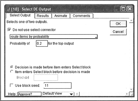
• The Select DE Output block from the Routing submenu of the Discrete Event library allows items in two different paths to be routed according to a variety of conditions. A common way of using this block is to model routing based on a probability value. This is done by checking the Do Not Use Connector box and then selecting the Route Items by Probability option. A probability value associated with the top output should be provided in the dialogue of this block.
• The Labor Pool block from the Resources submenu of the BPR library is used to introduce people as resource items in the model. The initial number of people is specified in the block’s dialogue window. The Labor Pool block keeps track of the utilization of the people in the resource pool.
• The Batch block from the Batching submenu of the Discrete Event library is used to batch up to three inputs into a single output. The number of required items from each input is specified in the dialogue window of this block.
• The Unbatch block from the Batching submenu of the Discrete Event library is used to unbatch items that have been batched previously with a Batch block. For example, a Batch block could be used to batch a job with the worker who is going to perform the job. When the worker completes the job, the Unbatch block can be used to separate the worker from the job and return the worker to a Labor Pool. When using the Batch and Unbatch blocks in this way, one must make sure that the Preserve Uniqueness box is checked in both blocks. Preserve Uniqueness appears in the first tab of the dialogue window of both blocks.

The blocks previously discussed are used to extend the current model as follows.

1. Add a Batch block, a Transaction block, and a Select DE Output block between the In Box block and the Underwriting block. Also add two Unbatch blocks, a Merge block, a Labor Pool block, and an Input Random Number block.
2. Connect the In Box block to the top input of the Batch block (named Batch block). Connect the output of the Labor Pool block (now named Teams block) to the bottom input of the Batch block. Then connect the output of the Batch block to the new Transaction block, now named Review block. Connect the blocks to make the model look like the one depicted in Figure 7.22. The model contains two named connections: Review Done and Underwriting Done. To make these connections, double-click where text is to be added. This opens a text box. Type the desired text and when finished typing, click anywhere else in the model or press Enter. The text box can now be connected to any block connector. Copy and paste the text box to establish the named connection.
3. In the dialogue window of the Batch block, enter a quantity of 1 for the top and the bottom outputs. Check the Preserve Uniqueness box. If one of the two incoming items is not available (such as if a request is waiting to be processed but there is no team ready), the Batch block does not release the batched item until both inputs come into the block.
4. In the dialogue window of the Teams block, set the initial number to 2.
5. The dialogue of the Select DE Output block labeled Approve? is depicted in Figure 7.23. The Do Not Use Select Connector box is checked, the Route Items by Probability option is selected, and the probability of 0.2 for the top output connector is specified.

    

   

   FIGURE 7.22 Underwriting Process Model with a Review Activity and a Labor Pool

    

   

   FIGURE 7.23 Dialogue Window for the Block Labeled “Approve?”

6. In the dialogue of the Unbatch blocks, enter a 1 in the Top and Bottom outputs. Also, check the Preserve Uniqueness box. This block separates the team from the request, and the team is sent back to the Labor Pool block.

The Input Random Number blocks in the model in Figure 7.22 are named after the probability distribution they simulate. For example, the Uni(0.25,0.5) block simulates a uniform distribution with parameters 0.25 and 0.5 to represent the number of hours to review a request. This means that in the dialogue of this block, the distribution “Real, uniform” is selected with Min = 0.25 and Max = 0.5. As in previous versions of this model, the Exp(0.8) simulates the exponential distribution with Mean = 0.8. After running the model in Figure 7.22, the following results are obtained.

• The utilization of the underwriting teams is approximately 51 percent.
• No requests are in the In Box at the end of the run, and the maximum number of requests throughout the simulation is seven. The average and maximum waiting times in the In Box are 0.123 and 4.9 hours, respectively.

Also, approximately 21 percent of the requests are rejected (836/3,989). This rejection rate is close to the assumed rejection rate of 20 percent.

7.7 Customizing the Animation

Model development and validation have always been considered key elements in computer simulations, but animation is gaining recognition as an additional key component. Extend offers extensive opportunities for customizing the animation in a model. The Animate Value, Animate Item, and Animate Attribute blocks, all from the Animation library, show customized animation in response to model conditions. Based on choices in their dialogues, these blocks can display input values, show a level that changes between specified minimums and maximums, display text or animate a shape when the input value exceeds a critical value, or change an item’s animation icon based on an attribute value. The blocks in this library can be used to develop models with sophisticated animation features, including pictures and movies.

A simple way of customizing the animation in a simulation model consists of changing the appearance of the items in the model. Turn on animation by selecting Run > Show Animation, and make sure that Add Connection Line Animation also is selected in the Run menu. When the simulation is run, Extend’s default animation picture, a green circle, will flow along the connection lines between blocks. In the Animate tab of blocks that generate items, such as the Import block named “Requests In” in this model, the animation picture that will represent the items generated by this block can be chosen. In the animation tab of the Requests In block, choose the paper picture to represent the requests as shown in Figure 7.24.

The request generated in the Requests In block will now appear as paper flowing through the model. Make sure that in the Animate tab of blocks that do not generate items but process them, the option Do Not Change Animation Pictures is selected.

The Teams block provides people for the review and underwriting activities. In the Animate tab of this Labor Pool block, choose the person picture to represent the teams. Because of how attributes are merged in the batching activity, the teams will inherit the animation picture of the requests (paper picture) while the two items remain batched. The items recover their original animation after they are unbatched. In the Teams block it is possible to make sure that all items are animated using the person picture by checking the “All Items Passing Through This Block Will Animate the Above Picture” option in the Animate tab, as depicted in Figure 7.25.

 

 

The model now shows the paper and person pictures when running the simulation in the animation mode.

7.8 Calculating Costs and Using the Flowchart View

Extend’s activity-based costing feature can help in calculating the cost of reviewing and underwriting. In this model, two things contribute to the total cost.

• The teams are paid $46.50 per hour. (Three team members each earn $15.50 per hour.)
• As part of the review activity, a report is generated that costs $25.

In the Cost tab of the Labor Pool block, fill in the cost per hour for the teams and select Resources in the Workers Used As: pop-up menu shown in Figure 7.26.

In the Cost tab of the Transaction block named Review, fill in the cost of the report (Cost per Item), as shown in Figure 7.27.

In the dialogue of both Unbatch blocks, choose the Release Cost Resources option. (See Figure 7.28.)

When the simulation is run, the costs are tracked with each request. To collect the cost data, add a Cost Stats block (from the Statistics submenu of the Discrete Event library) anywhere in the model and Cost by Item blocks (also from the Statistics submenu of the Discrete Event library) after the Unbatch blocks as shown in Figure 7.29.

The average cost per rejected request is approximately $42.21, and the average cost of a completed request is approximately $80.15. These values are given in the dialogue of the Cost by Item blocks at the end of the simulation run. This information provides the basis for setting the value for a possible application fee for this process. From the Cost Stats block, it also is known that the cost of this process is approximately $4,107 per week.

Figure 7.29 shows the simulation model using the classic view of Extend. Instead of this classic view, simulation models can be viewed using flowchart icons. This easy transformation is done by selecting Model > Change Icon Class > Flow Chart. The result of this change is shown in Figure 7.30.

 

 

 

 

A flowchart view such as the one shown in Figure 7.30 is particularly helpful in situations in which the simulation model is based on an existing flowchart of a process. The flowchart view allows a direct comparison between the model and the document that was used as the basis for the development of the simulation.

 

7.9 Summary

This chapter introduced the main discrete-event simulation functionality of Extend. A simple, one-stage process was used to illustrate how to model using block diagrams. The basic concepts discussed in this chapter are sufficient to model and analyze fairly complicated business processes. However, the full functionality of Extend goes beyond what is presented here and makes it possible to tackle almost any situation that might arise in the design of business processes.

7.10 References

Extend v6 User's Guide. 2002. Imagine That, Inc., San Jose, California.

7.11 Discussion Questions and Exercises

1. Consider a single-server queuing system for which the interarrival times are exponentially distributed. A customer who arrives and finds the server busy joins the end of a single queue. Service times of customers at the server are also exponential random variables. Upon completing service for a customer, the server chooses a customer from the queue (if any) in a first-in-first-out (FIFO) manner.
   1. Simulate customer arrivals assuming that the mean interarrival time equals the mean service time (e.g., consider that both of these mean values are equal to 1 minute). Create a plot of number of customers in the queue (y-axis) versus simulation time (x-axis). Is the system stable? (Hint: Run the simulation long enough [e.g., 10,000 minutes] to be able to determine whether or not the process is stable.)
   2. Consider now that the mean interarrival time is 1 minute and the mean service time is 0.7 minute. Simulate customer arrivals for 5,000 minutes and calculate: (i) the average waiting time in the queue, (ii) the maximum waiting time in the queue, (iii) the maximum queue length, (iv) the proportion of customers having a delay time in excess of 1 minute, and (v) the expected utilization of the server.
2. For the single-server queuing system in exercise lb, suppose the queue has room for only three customers, and that a customer arriving to find that the queue is full just goes away. (This is called balking.) Simulate this process for 5,000 minutes, and estimate the same quantities as in part b of exercise 1, as well as the expected number of customers who balk.
3. A service facility consists of two servers in series (tandem), each with its own FIFO queue. (See Figure 7.31.) A customer completing service at server 1 proceeds to server 2, and a customer completing service at server 2 leaves the facility. Assume that the interarrival times of customers to server 1 are exponentially distributed with mean of 1 minute. Service times of customers at server 1 are exponentially distributed with a mean of 0.7 minute, and at server 2 they are exponentially distributed with a mean of 0.9 minute.
   1. Run the simulation for 1,000 minutes and estimate for each server the expected average waiting time in the queue for a customer and the expected utilization.
   2. Suppose that there is a travel time from the exit of server 1 to the arrival to queue 2 (or server 2). Assume that this travel time is distributed uniformly between 0 and 2 minutes. Modify the simulation model and run it again to obtain the same performance measures as in part a. (Hint: You can add a Transaction block to simulate this travel time. A uniform distribution can be used to simulate the time.)

       

      

      FIGURE 7.31 Process with Two Servers in Series

   3. Suppose that no queuing is allowed for server 2. That is, if a customer completing service at server 1 sees that server 2 is idle, the customer proceeds directly to server 2, as before. However, a customer completing service at server 1 when server 2 is busy with another customer must stay at server 1 until server 2 gets done; this is called blocking. When a customer is blocked from entering server 2, the customer receives no additional service from server 1 but prevents server 1 from taking the first customer, if any, from queue 1. Furthermore, new customers may arrive to queue 1 during a period of blocking. Modify the simulation model and rerun it to obtain the same performance measures as in part a.
4. A bank with five tellers opens its doors at 9 A.M. and closes its doors at 5 P.M., but it operatesuntil all customers in the bank by 5 P.M. have been served. Assume that the interarrival times of customers are exponentially distributed with a mean of 1 minute and that the service times of customers are exponentially distributed with a mean of 4.5 minutes. In the current configuration, each teller has a separate queue. (See Figure 7.32.) An arriving customer joins the shortest queue, choosing the shortest queue furthest to the left in case of ties.

   The bank’s management is concerned with operating costs as well as the quality of service currently being provided to customers and is thinking of changing the system to a single queue. In the proposed system, all arriving customers would join a single queue. The first customer in the queue goes to the first available teller. Simulate 5 days of operation of the current and proposed systems and compare their expected performance.

5. Airline Ticket Counter—At an airline ticket counter, the current practice is to allow queues to form before each ticket agent. Time between arrivals to the agents is exponentially distributed with a mean of 5 minutes. Customers join the shortest queue at the time of their arrival. The service time for the ticket agents is uniformly distributed between 2 and 10 minutes.
   1. Develop an Extend simulation model to determine the minimum number of agents that will result in an average waiting time of 5 minutes or less.
   2. The airline has decided to change the procedure involved in processing customers by the ticket agents. A single line is formed and customers are routed to the ticket agent who becomes free next. Modify the simulation model in part a to simulate the process change. Determine the number of agents needed to achieve an average waiting time of 5 minutes or less.
   3. Compare the systems in parts a and b in terms of the number of agents needed to achieve a maximum waiting time of 5 minutes.
   4. It has been found that a subset of the customers purchasing tickets is taking a long period of time. By separating ticket holders from nonticket holders, management believes that improvements can be made in the processing of customers. The time needed to check in a person is uniformly distributed between 2 and 4 minutes. The time to purchase a ticket is uniformly distributed between 12 and 18 minutes: Assume that 15 percent of the customers will purchase tickets and develop a model to simulate this situation. As before, the time between all arrivals is exponentially distributed with a mean of 5 minutes. Suggest staffing levels for both counters, assuming that the average waiting time should not exceed 5 minutes.

       

      

      FIGURE 7-32 Teller Configuration (multiple queues)

6. Inventory System—A large discount store is planning to install a system to control the inventory of a particular video game system. The time between demands for a video game system is exponentially distributed with a mean time of 0.2 weeks. In the case where customers demand the system when it is not in stock, 80 percent will go to another nearby discount store to find it, thereby representing lost sales; the other 20 percent will backorder the video system and wait for the arrival of the next shipment. The store employs a periodic review-reorder point system whereby the inventory status is reviewed every 4 weeks to decide whether an order should be placed. The company policy is to order up to the stock control level of 72 video systems whenever the inventory position, consisting of the systems in stock plus the systems on order minus the ones on backorder, is found to be less than or equal to the reorder point of 18 systems. The procurement lead time (the time from the placement of an order to its receipt) is constant and requires 3 weeks. Develop an Extend model to simulate the inventory policies for a period of 6 years (312 weeks) to obtain statistics on (a) the number of video systems in stock, (b) the inventory position, (c) the safety stock (the number of video systems in stock at the time of receiving a new order), and (d) the number of lost sales. Investigate improvements on this inventory policy by changing the reorder point, the stock control level, and the time between reviews.
7. Bank Tellers—Consider a banking system involving two inside tellers and two drive-in tellers. Arrivals to the banking system are either for the drive-in tellers or for the inside tellers. The time between arrivals to the drive-in tellers is exponentially distributed with a mean of 1 minute. The drive-in tellers have limited waiting space. Queuing space is available for only three cars waiting for the first teller and four cars waiting for the second teller. The service time of the first drive-in teller is normally distributed with a mean of 2 minutes and a standard deviation of 0.25. The service time of the second drive-in teller is uniformly distributed between 1 minute and 3 minutes. If a car arrives when the queues of both drive-in tellers are full, the customer balks and seeks service from one of the inside bank tellers. However, the inside bank system opens 1 hour after the drive-in bank, and it takes between 0.5 and 1 minute to park and walk inside the bank. Customers who seek the services of the inside tellers directly arrive through a different process, with the time between arrivals exponentially distributed with a mean of 1.5 minutes. However, they join the same queue as the balkers from the drive-in portion. A single queue is used for both inside tellers. A maximum of seven customers can wait in this single queue. Customers arriving when seven are in the inside queue leave. The service times for the two inside tellers are triangularly distributed between 1 and 4 minutes with a mode of 3 minutes. Simulate the operation of the bank for an 8-hour period (7 hours for the inside tellers). Assess the performance of the current system.
8. Grocery Store—You are hired by Safeway to help them build a number of simulation models to better understand the customer flows and queuing processes in a grocery store setting. The pilot project at hand focuses on an off-peak setting where at most two checkouts are open. To better understand the necessary level of detail and the complexities involved, Safeway wants a whole battery of increasingly more realistic and complex models. For each model, Safeway wants to keep track of (i.e., plot) the average cycle time, queue length, and waiting time in the queue. To understand the variability, they also want to see the standard deviation of these three metrics. In addition, they would like to track the maximum waiting time and the maximum number of customers in line. Furthermore, to better understand the system dynamics, plots of the actual queue lengths over time are required features of the model. The off-peak setting is valid for about 4 hours, so it is reasonable to run the simulation for 240 minutes. Furthermore, to facilitate an easier first-cut comparison between the models, a fixed random seed is recommended. Because Safeway plans to use these different models later, it is important that each model sheet has a limn of one model.
   1. In the first model, your only interest is the queues building up at the checkout counters. Empirical investigation has indicated that it is reasonable to model the arrival process (to the checkout counters) as a Poisson process with a constant arrival intensity of three customers per minute. The service time in a checkout station is on average 30 seconds per customer and will, in this initial model, be considered constant. Inspired by the successes of a local bank, Safeway wants to model a situation with one single line to both checkout counters. As soon as a checkout is available, the first person in the queue will go to this counter. After the customers have paid for their goods, they immediately leave the store.
   2. Upon closer investigation, it is clear that the service time is not constant but rather normally distributed with μ = 30 seconds and σ = 10 seconds. What is the effect of the additional variability compared to the results in part a?
   3. To be able to analyze the effect of different queuing configurations, Safeway wants a model in which each checkout counter has its own queue. When a customer arrives to the checkout point, he or she will choose the shortest line. The customer is not allowed to switch queues after making the initial choice. Can you see any differences in system performance compared to the results in part b?