Reflections, refractions, and chromatic aberrations are important qualities of materials such as water and glass. The Maya Software and mental ray renderers can provide these qualities through the raytracing process. Although the two renderers share many attributes, mental ray offers many advanced features. In particular, mental ray provides greater flexibility when rendering shadows and motion blur.
Chapter Contents
Raytracing with the Maya Software renderer
Creating reflections, refractions, and chromatic aberrations
Motion blur and shadows with mental ray
Raytracing with the mental ray renderer
Reproducing water and glass with Maya Software and mental ray
By default, Maya renders with the Maya Software renderer. You can switch to the Maya Hardware, Maya Vector, or mental ray renderer by changing the Render Using attribute in the Render Settings window. Although the Maya Hardware and Maya Vector renderers are designed for specialized rendering situations, mental ray can easily handle renders normally tackled by Maya Software. As such, the advantages of Maya Software and mental ray renderers may not be immediately obvious. Therefore, I've included a short list for each:
Maya Software
Supports the Studio Clear Coat plug-in (Chapter 7)
Renders rapidly while providing attributes for high-quality anti-aliasing (Chapter 10)
Offers relatively few attributes and is thus easy to set up (Chapter 10)
mental ray
Includes Maya Fur and the Maya Hair system in reflections and refractions (Chapter 3)
Renders bump maps with greater accuracy (Chapter 9)
Is able to motion blur shadows (this chapter)
Is able to impart transparency to depth map shadows (this chapter)
Provides Global Illumination and Final Gather rendering options (Chapter 12)
Utilizes Maya shaders as well as mental ray shaders (Chapter 12)
Although mental ray's list of advantages is quite long, Maya Software is perfectly suitable for many renders. The trick is to become familiar with both systems so that you can make appropriate decisions at render time.
By default, the Maya Software renderer operates in a scanline mode. To activate raytracing, check the Raytracing attribute in the Raytracing Quality section of the Maya Software tab in the Render Settings window (see Figure 11.1).

Before I describe the raytracing process in more detail, the scanline process is worth a closer look. In general, the scanline process is as follows:
The renderer examines the objects in the scene. The objects within the camera frustum are added to a list and their bounding boxes are calculated.
The image to be rendered is divided into tiles to optimize memory usage. The complexity of the objects within a tile determines the tile's size.
Polygon triangles associated with visible objects are processed in scanline order. Each triangle is projected into screen space and is clipped to the boundaries of each pixel it covers. That is, the portions of the triangle outside the pixel boundaries are temporarily discarded. Each pixel is thus given a list of clipped triangle fragments. The fragments are stored in the lists as bit masks, which are binary representations of fragment visibility within a pixel. The algorithm responsible for this process is known as A-buffer.
The colors of each fragment are derived from the material qualities of the original polygons and the influence of lights in the scene. The final color of the pixel is determined by averaging the fragment colors, with emphasis given to those fragments that are the most visible. As part of this process, fragments are depth-sorted and additional clipping is applied to those fragments that are occluded.
By comparison, the raytracing process fires off a virtual ray from the camera eye through each pixel of a view plane (see Figure 11.2). The number of pixels in the view plane corresponds to the number of pixels required for a particular render resolution.
The first surface the ray intersects determines the pixel's color. That is, the material qualities of the surface are used in the shading calculation of the pixel. If raytrace shadows are turned on, secondary shadow rays are fired from the point of intersection to each shadow-producing light. If a shadow ray intersects another object before reaching a particular light, then the original intersection point is shadowed by that object. If the first surface is reflective and/or refractive, additional rays are created at the original intersection point. One ray represents the reflection, and the other represents the refraction. If either ray intersects a secondary reflective and/or refractive surface, the ray-splitting process is repeated. This continues until the rays reach a predefined, maximum number of reflection and refraction intersections. When a reflection ray reaches a secondary surface, the shading model of the secondary surface is calculated and contributed to the original intersection point. Hence, the color of secondary surface appears on the original surface as a reflection. A similar process occurs with a refraction ray, whereby the secondary surface shading model is contributed to the original intersection point. However, the direction that the refraction ray travels in is influenced by the Refractive Index (which is discussed later in this chapter).

Because a single camera eye ray can easily produce numerous shadow, reflection, and refraction rays, raytrace rendering is significantly more complex than the equivalent render with the scanline process. Consequently, the Maya Software renderer combines the scanline and raytrace techniques. If Raytracing is checked on but a surface possesses no reflective or refractive qualities, Maya applies the scanline process and avoids tracing rays.
Another method by which Maya reduces raytrace calculations is through the creation of voxels. Voxels are virtual cubes created from the subdivision of a scene's bounding box (which includes all objects within the scene). Maya tests for ray intersections with voxels before calculating more exact surface intersections. This effectively reduces the number of surfaces that are involved with the intersection calculations. Without voxels, Maya would have to test every surface in a scene.
The Ray Tracing subsection of the Memory And Performance Options section in the Maya Software tab controls voxel creation through Recursion Depth, Leaf Primitives, and Subdivision Power attributes.
- Recursion Depth
Sets the number of available recursive levels of voxel subdivision. Values of 1 to 3 work for most scenes, with complex setups requiring higher numbers.
- Leaf Primitives
Defines the maximum number of polygon triangles permitted to exist in a voxel before it is recursively subdivided.
Recursive subdivisions occur locally. Thus, if a voxel is subdivided, the resulting subvoxels are tested for subdivision. If the subvoxels are subdivided into sub-subvoxels, the sub-subvoxels are tested for subdivision. This process continues until all resulting voxels contain a number of triangles that is less than the Leaf Primitives value. At the same time, many of the original voxels and subvoxels may escape subdivision because they always contained a number of triangles less than the Leaf Primitives value.
For example, if Leaf Primitives is set to 200 and a tested voxel contains 1,000 triangles, the voxel is subdivided into 8 subvoxels. Each of the subvoxels is tested. If any single subvoxel possesses more than 200 triangles, it is subdivided into 8 sub-subvoxels.
For efficiency, the number of times a voxel is recursively subdivided is curtailed by the Subdivision Power attribute. In addition, the Recursion Depth attribute sets a cap on the number of available recursive steps.
- Subdivision Power
The power by which the number of polygon triangles in a voxel is raised to determine how many times the voxel should be recursively subdivided (if recursion is deemed necessary by the Leaf Primitives attribute). For example, if there are 1,000 triangles in a voxel, and the Subdivision Power value is changed from 0.25 to 0.5, the following math occurs:
1000 ^ 0.25 = 5.62
1000 ^ 0.5 = 31.62
Large Subdivision Power values lead to large results, which in turn create a greater number of recursive subdivisions and a greater number of subdivided voxels. Small subvoxels are inefficient if the majority of their brethren are wasted on empty space. On the other hand, a limited number of large subvoxels are also inefficient if they contain a high number of triangles.
Since Subdivision Power is not intuitive, it's best to change the attribute value by small increments. Maya documentation recommends a setting of 0.25 for most scenes.
The Raytracing Quality section of the Maya Software tab provides Reflections, Refractions, Shadows, and Bias attributes. The Reflections attribute sets the maximum number of times a camera eye ray will generate reflection rays before it is killed off. The Refractions attribute sets the maximum number of times a camera eye ray will generate refraction rays before it is killed off (see Figure 11.3). The limit for both attributes is 10, which is satisfactory for a water glass, bottle, or vase.

Figure 11.3. Rays generated by a single camera eye ray while the Reflections and Refractions attributes are set to 2
The Shadows attribute, on the other hand, sets the maximum number of times a camera eye ray can reflect and/or refract and continue to generate shadow rays. The higher the value, the more recursive the shadows; that is, shadows will appear within reflections of reflections and refractions of refractions. This attribute only has an effect if raytraced shadows are used. Depth map shadows, whether they are generated by Maya Software or mental ray, will automatically show up in all recursive reflections. If Shadows is set to 0, all raytrace shadows are turned off. A value of 10 will render shadows within nine recursive levels of reflection or refraction (see Figure 11.4). If Shadows is set to 10 and no raytrace shadows appear in reflections or refractions, increase the Ray Depth Limit attribute in the Raytrace Shadow Attributes subsection of the light's Attribute Editor tab. (See Chapter 3 for more detailed information.)
The Bias attribute serves as an adjustment for 3D motion blur in scenes with raytrace shadows. Often, raytrace shadows create dark bands around the center of rapidly moving objects. You can increase the Bias value to remove this artifact (see Figure 11.5).


As soon as the Raytracing attribute is checked, the Maya Software renderer creates reflections for all objects. The amount of reflectivity is controlled on a per-material basis by the material's Reflectivity attribute. This attribute works in conjunction with the Specular Roll Off and Specular Color attributes. If Specular Roll Off and Specular Color are set to 0, there is no reflection. A material's Eccentricity attribute, on the other hand, has no effect on the strength of a reflection and can be set to 0.
Note
Anisotropic materials carry an Anisotropic Reflectivity attribute, which overrides the standard Reflectivity attribute when checked. With Anisotropic Reflectivity, the strength of the reflection is determined by the Roughness attribute. The higher the Roughness value, the dimmer the reflection.
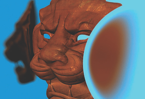
In contrast, the Reflected Color attribute found on Blinn, Phong, Phong E, and Anisotropic materials does not require raytracing. If the Reflected Color value is set to a color other than black or is mapped, a simulated reflection is applied directly to the assigned surface. If the mapped texture is an environment texture, the results are quite convincing (see Chapter 5 for a demonstration). Although a raytraced reflection is more accurate than a texture mapped to the Reflected Color attribute, raytracing is considerably less efficient. In any case, you can map the Reflected Color attribute and raytrace at the same time (see Figure 11.6). The color of light reflected in the raytrace process is multiplied by the Reflected Color attribute.
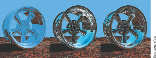
Figure 11.6. (Left) Raytraced chrome rim with the camera's Background Color set to blue. (Middle) Same rim with an environment texture mapped to the Reflected Color attribute, but without raytracing. (Right) Same rim with an environment texture and raytracing.
The Reflection Limit attribute (found in a material's Raytrace Options section) is a per-material attribute that sets the number of times a camera eye ray is allowed to reflect off the assigned surface before it is killed. Maya will compare the Reflection Limit to the Reflections attribute in the Raytracing Quality section of the Maya Software tab and use the lower value of the two.
The Reflection Specularity attribute (also found in a material's Raytrace Options section) controls the contribution of specular highlights to reflections. For example, in Figure 11.7 a car rim is assigned to two materials. The spokes are assigned to a red Blinn with its Reflection Specularity set to 0. The outer rim is assigned to a gray Blinn with its Reflection Specularity set to the default 1. Thus, the reflection of the spokes in the rim does not include the specular component. However, if the spoke's Reflection Specularity is returned to 1, the specular highlights of the spokes become visible in the rim reflection. When set to a value below 1, the Reflection Specularity attribute can help reduce anti-aliasing artifacts resulting from recursive reflections that contain a high degree of detail.

Refraction is the change in direction of a light wave due to a change of speed. When a light wave crosses the boundary between two materials with different refractive indices, its speed and direction are shifted. The human brain, unaware of this shift, assumes that all perceived light travels in a straight line. Thus, refracted light is perceived to originate from an incorrect location and objects appear bent or distorted. (For more detailed information on refractive indices, see Chapter 7.)
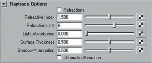
In Maya, refractions are defined on a per-material basis in the Raytrace Options section of the material's Attribute Editor tab. Refraction attributes include Refractive Index, Refraction Limit, Light Absorbance, Surface Thickness, Shadow Attenuation, and Chromatic Aberration (See Figure 11.8).
- Refractive Index
Sets the refractive index of the assigned surface. The index is a constant that relates the speed of light through a vacuum and the speed of light through a particular material. In the real world, the refractive index of water is approximately 1.33, and glass varies from 1.45 to 1.85. The default value of 1 creates no refraction and is the same as air.
- Refraction Limit
Sets the per-material maximum number of times a camera eye ray is refracted through the assigned surface before it is killed off. Maya compares this attribute to the Refractions attribute in the Raytracing Quality section of the Maya Software tab and uses the lower of the two.
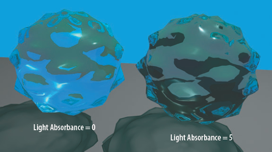
- Light Absorbance
Describes the amount of light that is absorbed by transparent or semitransparent objects. All real-world materials absorb light at different wavelengths (in which case the light energy is converted to heat). When set to 0, the Light Absorbance attribute allows 100 percent of the light to pass through the object. The higher the value, the more light is absorbed by the object's surface and the darker the surface appears (see Figure 11.9).
- Surface Thickness
Determines the simulated thickness of a surface that possesses no model thickness. For example, in Figure 11.10 two primitive NURBS planes are given different Surface Thickness values. Since the left NURBS plane has a Surface Thickness value of 100, the sky color is not visible in its refraction; in addition, the high value creates a magnifying glass effect, which enlarges the table's checker pattern.
- Shadow Attenuation
Replicates the brightening of a shadow's core and the darkening of the shadow's edge when the shadow is cast by a semitransparent object. A high Shadow Attenuation value creates a high-contrast transition within the shadow (see Figure 11.11). A value of 0 turns the Shadow Attenuation off. The Refractions attribute does not have to be checked for Shadow Attenuation to work.

Figure 11.10. The refraction of a NURBS plane is adjusted with the Surface Thickness attribute. This scene is included on the CD as
thickness.ma.
Figure 11.11. A high Shadow Attenuation attribute value creates greater contrast within the shadow. This scene is included on the CD as
attenuation.ma.You can also use the Shadow Attenuation attribute to adjust raytraced shadows that involve materials with Transparency maps. If Shadow Attenuation is left at the default value of 0.5, the part of the Transparency map that is 100 percent white will sometimes cast a soft shadow. At other times, a high Attenuation value may cause the shadow artifact to appear. For example, in Figure 11.12 a directional light casts the shadow of a plane that has a bitmap of a star symbol mapped to its material's Transparency attribute. The black lines in the figure represent the position of the shadowed plane. The red lines represent the edges of the plane as they appear as part of the shadow. The area within the red lines is darkened slightly, even though the Transparency map should provide nothing to shadow around the edges of the star. In this case, Attenuation is set to 1. When Attenuation is reduced to 0, however, the darkened area disappears appropriately.
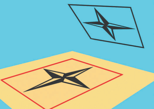
Figure 11.12. A Transparency map applied to the material of a plane casts a raytraced shadow. The red lines represent the edges of the plane as they appear as part of the shadow. An adjustment of the Attenuation attribute can prevent this area from rendering inappropriately dark. This scene is included on the CD as
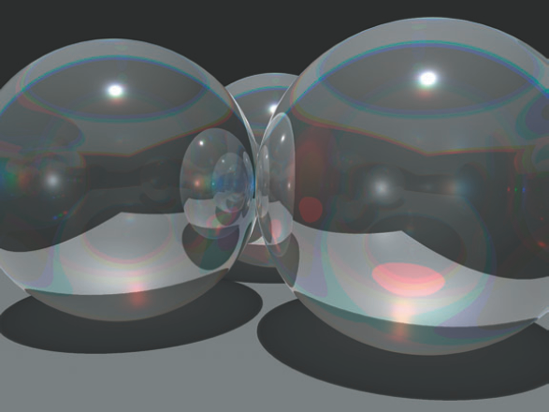
attenuation_trans.ma.- Chromatic Aberration
Refers to the inability of a lens to equally focus different color wavelengths. This is an artifact of dispersion, in which different wavelengths of light travel through a medium, such as glass, at different speeds. In effect, this causes a lens to have a different refractive index for each wavelength. Maya's Chromatic Aberration attribute distorts refraction rays, causing colors to shift as shading models are invoked. Points closer to the light source shift toward cyan, while points farther from the light shift toward red and yellow (see Figure 11.13). The aberration is only visible if the Refractions attribute is checked.
By default, the mental ray renderer operates in scanline mode. Raytracing is only employed if it is activated as a secondary effect.
Since many mental ray attributes are unique—or at least different in name—it is worth examining some common settings in the Render Settings window. As part of this review, mental ray motion blur and shadows are detailed.
The mental ray Quality Presets attribute, found in the mental ray tab of the Render Settings window, supplies 15 different presets. The presets offer a quick way to set all the attributes within the Rendering Features and Anti-Aliasing Quality sections (see Figure 11.14). For instance, if you set Quality Presets to Draft, the Primary Renderer is set to Scanline and anti-aliasing is kept at a bare minimum to speed the render. If you set Quality Presets to Preview: Global Illumination, Raytracing and Global Illumination is checked for the Secondary Effects attribute; in addition, matching Global Illumination attributes found in the Caustics And Global Illumination section are set to a quality appropriate for a preview. For maximum control, you can set all the Rendering Features and Anti-Aliasing Quality attributes by hand. Descriptions of each attribute follow:
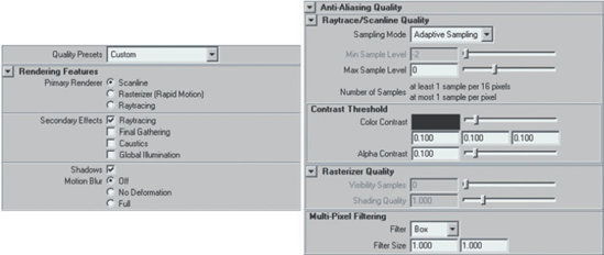
Figure 11.14. The Rendering Features section (Left) and Anti-Aliasing Quality section (Right) of the mental ray tab in the Render Settings window
- Primary Renderer
Chooses the primary renderer. The Scanline option rapidly renders simple scenes. The Rasterizer (Rapid Motion) option, however, is more efficient when the scene is complex or has numerous motion blurred objects. (The Rasterizer option was previously named Rapid Scanline.) The Raytracing option forces the entire scene to be raytraced. The Raytracing option, by itself, will not produce reflections and refractions—the Raytracing option of the Secondary Effects attribute must be checked.
Note
The Rasterizer (Rapid Motion) primary renderer treats motion blur in a more efficient manner than the Scanline primary renderer. Instead of sampling and shading each visible point of a moving object multiple times along its motion path for a single frame, the Rasterizer samples all objects at a fixed position. The shading information is cached, and then is allowed to "travel" with the object when it is placed at the end of its motion path for a particular frame. Because each visible point has only one shading sample taken per frame, the calculation time is sped up significantly.
- Secondary Effect
Toggles on and off Raytracing, Final Gathering, Caustics, and Global Illumination. Secondary infers that the effects are only employed at a point deemed necessary by the primary renderer.
- Shadows and Motion Blur
Shadows serves as a master on/off switch for all raytrace and depth map shadows. Motion Blur determines whether motion blur is off or on and chooses the No Deformation or Full method. (See the next section for more information.)
- Sampling Mode
Sets the style of anti-aliasing sampling. The Fixed Sampling option uses a static number of subpixel samples per pixel. The Adaptive Sampling and Custom Sampling options use a different number of subpixel samples per pixel based on the contrast within the scene. Although Adaptive Sampling allows you to adjust the Max Sample Level attribute directly, Custom Sampling lets you adjust both the Min Sample Level and Max Sample Level attributes. (For more information on anti-aliasing, see Chapter 10.)
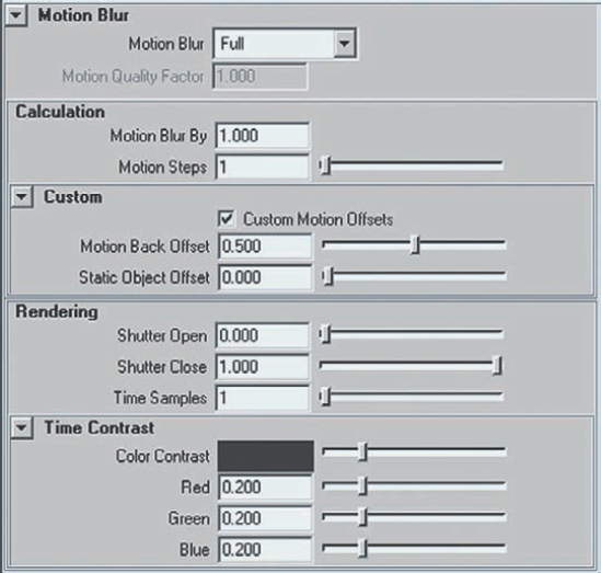
- Color Contrast
A "dummy" attribute that drives Contrast R, Contrast G, and Contrast B attributes. The values of Contrast R, Contrast G, and Contrast B are listed in the three cells below the Color Contrast slider. You can change the values in the cells by hand. Contrast R, Contrast G, and Contrast B set the contrast threshold for subpixel sampling when Sampling Mode is set to Adaptive Sampling or Custom Sampling. If a pixel, when compared to neighboring pixels, does not exceed the contrast threshold set by Contrast R, Contrast G, or Contrast B, the pixel is only sampled one time (assuming that Min Sample Level is set to 0). If the contrast threshold is exceeded, however, the pixel is subdivided and four subpixel samples are employed instead of one. The functionality of this section is similar to the Maya Software Contrast Threshold section, but provides the addition of an alpha channel contrast threshold slider (Alpha Contrast).
- Min Sample Level and Max Sample Level
Sets the minimum and maximum number of times a pixel is permitted to be recursively subdivided into subpixel samples. A value of 0 equates to one sample per pixel (in other words, no subpixel samples). When Sampling Mode is set to Custom Sampling, you can set the Min Sample Level to a negative number. In essence, this forces the renderer to skip some pixels in the pixel sampling process. For example, a value of −2 will force the renderer to take only one sample per block of 16 pixels. In contrast, a Max Sample Level value of 2 allows the renderer to sample each pixel 16 times. Hence, a Min Sample Level value of −2 and a Max Sample Level value of 0 is a low-quality render. A Min Sample Level value of 0 and a Max Sample Level value of 2 is a high-quality render. Remember that Min Sample Level and Max Sample Level set a range. The precise values derived from the range, and hence the number of subpixel samples used for a particular pixel, are controlled by the Color Contrast values.
As a simplified example of the sampling process, the following steps occur for a theoretical block of four pixels:
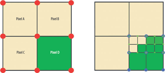
Min Sample Level is set to 0. Max Sample Level is set to 2. Because Min Sample Level is 0, the 4 pixels are sampled (and not skipped). With mental ray, each pixel is sampled at its four corners to determine the pixel color (see Figure 11.15).
The contrast between pixels sharing corners is tested. For instance, Pixel B has a Red value of 0.9. Pixel D has a Red value of 0.3. The difference between the two values is 0.6. Since Contrast R is set to 0.25 and 0.6 is greater than 0.25, Pixel D is subdivided into 4 subpixels.
The color of each new subpixel is determined and tested against subpixels sharing its corners. If the contrast threshold is exceeded for any subpixel, the subpixel is subdivided into sub-subpixels. The recursive subdivision stops at the sub-subpixel level, however, because the Max Sample Level is set to 2, which limits the maximum number of subpixels samples per pixel to 16. You can write the math like so:
4 subpixels × 4 sub-subpixels = 16
All the subpixels and sub-subpixels are tested before the renderer moves on to the next pixel. This process also requires the testing of the Green, Blue, and Alpha channels.
Note
The Contrast Threshold section is not available to the Rasterizer (Rapid Motion) primary renderer. Instead, Visibility Samples and Shading Quality are available in the Rasterizer Quality section. Visibility Samples sets the number of subpixel samples used in the anti-aliasing process (a value of 0 defaults to four corner samples per pixel). Shading Quality increases or decreases the number of subpixel samples used in the shading process.
- Filter and Filter Size
The Filter attribute determines the style of multipixel filter used by the renderer. Multipixel filtering is designed to blend neighboring pixels together into a coherent mass. Such filtering helps to prevent aliasing in the form of buzzing or stair-stepping. You can choose from five styles. Gauss (Gaussian) produces the most thorough averaging but is the slowest to render. Box, on the other hand, is less processor intensive while producing acceptable results. Triangle is similar to Box but produces more accurate results. Mitchell and Lanczos are variations of Gauss that produce a greater degree of contrast. The Filter Size fields, which represent Filter Size X and Filter Size Y attributes, control the intensity of the pixel averaging. As the values are increased, the number of neighboring pixels that are included in the calculation is increased. The greater the number of pixels included in the calculation, the more accurate the averaging. High values may lead to excessive blurriness within the image, however. Unfortunately, the multipixel filter effect in mental ray cannot be turned off. However, Filter Size X and Filter Size Y can be set to 0.01, which makes the filter's impact negligible.
- Jitter and Sample Lock
Jitter, when checked, introduces systematic variations in subpixel sampling locations within pixels. Sample Lock, when checked, ensures that the sampling pattern is consistent across multiple frames of an animation. Sample Lock overrides Jitter. If neither attribute is checked, samples are taken at pixel corners. Although the default settings (Jitter off and Sample Lock on) for these attributes work in most situations, nondefault settings (such as Jitter on and Sample Lock off) may help solve anti-aliasing problems that other attributes fail to address.
You can access additional sampling attributes on a per-surface basis in the Render Stats section of a surface's Attribute Editor tab. If you check Shading Samples Override, Shading Samples and Max Shading Samples become available. These two attributes override Min Sample Level and Max Sample Level for the selected surface, but function in the same manner.
Two forms of motion blur are employed by the mental ray renderer: No Deformation and Full (respectively named Linear and Exact in previous versions). No Deformation motion blur is equivalent to Maya Software's 2D motion blur, in that it is unable to accurately portray rapid changes in direction or surface deformation. Full motion blur, on the other hand, plots the motion vectors of each surface vertex and is thus sensitive to deformation. (Unfortunately, Full motion blur handles rapid changes in direction in a fashion similar to No Deformation motion blur.) Attributes for mental ray motion blur are located in the Motion Blur section of the mental ray tab and include Shutter Open, Shutter Close, Motion Back Offset, and Static Object Offset, Motion Blur By, and Motion Steps (see Figure 11.16).
- Shutter Open and Shutter Close
Sets the points at which the virtual shutter opens and closes within the time interval of the frame. If the default values of 0 and 1 are kept, the motion blur calculation utilizes the entire time interval. For example, if the Maya scene file is set to 30 frames-per-second, the object is allowed to travel an appropriate distance for 1/30th of a second, which is indicated by the motion blur trail. If Shutter Open is raised and Shutter Close is reduced, the blur trail becomes shorter as the object is given less time to move for the purpose of motion blur calculation. Prior versions of Maya used Shutter and Shutter Delay for the same purpose.
- Motion Back Offset
Determines the time interval for the frame examined for motion blur. The default setting of 0.5 causes the renderer to go back in time 0.5 frames to establish the object's start position and forward in time 0.5 frames to determine the object's end position. This jumping back-and-forth in time is visible on the Timeline. When a frame is rendered through the Render View window, the Timeline will automatically hop from the start position frame to the end position frame during the render. However, the size of the hop does not match the Motion Back Offset value exactly. This is due to the following math:
Time Offset = ((((Shutter Close - Shutter Open) * Shutter Angle) / 360) * Motion
Blur By) * Motion Back Offset
In this case, Time Offset is a variable that represents the size of the Timeline "hop." If all the motion blur attributes are left at their default, the Timeline moves −0.2 frames to the start position and 0.2 frames to the end position. The Shutter Angle attribute, found in the Special Effects section of the rendered camera's Attribute Editor tab, is part of the equation and emulates the setup of a real-world motion picture camera.
- Motion Blur By
Serves as a multiplier for the motion blur effect. The larger the value, the more exaggerated the motion blur.
- Static Object Offset
Determines the time used to render static objects. A default value of 0 uses the current frame. Other values allow the renderer to go backward or forward in time to select shading samples for objects that have no animation. Static Object Offset and Motion Back Offset are only available if Custom Motion Offsets is checked.
- Motion Steps
Sets the number of motion vector segments that are created for moving objects. The higher the value, the more accurate the motion blur.
By default, mental ray motion blur appears extremely grainy. You can remedy this, however, by adjusting the Time Samples attribute (see Figure 11.17).
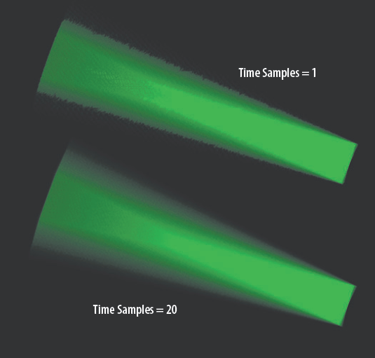
Figure 11.17. Motion blurred stick with two different Time Samples settings. This scene is included on the CD as mental_motion.ma.
In actuality, Time Samples is a "dummy" attribute that remotely controls the Time Contrast R, Time Contrast B, and Time Contrast G attributes found in the Time Contrast subsection (these are simply labeled Red, Green, and Blue in Maya 2008). Color Contrast, found in the same subsection, also serves as a dummy remote for Time Contrast R, Time Contrast B, and Time Contrast G. Ultimately, the Time Contrast attributes determine the number of temporal samples taken per spatial sample. For example, if the Time Contrast attributes are each set to 0.5, then 2 temporal samples are taken per spatial sample per frame. This equates to the formula 1 / Time Contrast.
Shadows created by mental ray are defined in two areas—the Shadows section of the mental ray tab in the Render Settings window and the shadow-specific sections of each light's Attribute Editor tab.
A light's Use Ray Trace Shadows attribute functions in the same manner for the mental ray renderer as it does for the Maya Software renderer. (Maya Software shadows are discussed in Chapter 3.) However, mental ray supplies separate attributes in the Shadows section of the mental ray tab in the Render Settings window (see Figure 11.18). The Shadow Method attribute controls the method of shadow calculation and has four options: Disabled, Simple, Sorted, Segments. The Simple method creates fast, efficient shadows and is appropriate for most animation. The Sorted method determines shadow order if multiple objects obscure the rendered point from the point-of-view of the shadowing light. With the Simple and Sorted method, shadow rays are generated by the light from the light's origin. Unless a custom mental ray shader is used, Sorted offers no advantage over Simple. The Segments method provides a more sophisticated model whereby shadow rays are traced from the rendered point back to the shadowing light. When the shadow ray strikes an obscuring object, it is terminated and a new shadow ray is born at the intersection. The new shadow ray continues toward the shadowing light (unless it too strikes an object). Each shadow ray, referred to as a shadow "segment," invokes a shadow shader. The Segments method is necessary if software-rendered particles or other volume effects require shadows. The Disabled option turns off shadows.

Raytrace shadows, by their very nature, understand object transparency. However, if depth map shadows are used with the mental ray renderer, object transparency information is ignored. This holds true for standard Maya depth maps, controlled by the Depth Map Shadow Attributes section of a light's Attribute Editor tab, as well as mental ray shadow maps, controlled by the mental ray section of a light's Attribute Editor tab. (For more information on depth map shadows, see Chapter 3.) Nevertheless, you can impart transparency to the depth map shadows by adjusting the Format attribute in the Shadows section of the mental ray tab in the Render Settings window.
If the Format attribute is set to Detail, mental ray takes into account surface properties, such as transparency, when building the shadows (see Figure 11.19). In addition, the Detail option provides superior depth map shadows for motion-blurred objects. If Use Ray Trace Shadows is checked in a light's Attribute Editor tab, the Format option is ignored for that light.
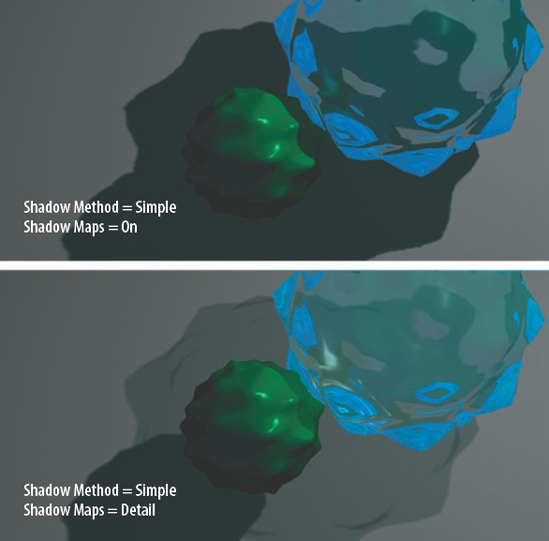
Figure 11.19. A mental ray shadow map with and without the Detail option. This scene is included on the CD as mental_detail.ma.
You can also access the Detail option through the mental ray section of a spot, point, or directional light's Attribute Editor tab. If you switch the Shadow Map Format attribute from Regular Shadow Map to Detail Shadow Map, the light overrides the Format attribute in the Shadows section of the mental ray tab of the Render Settings window. When selected, the Detail Shadow Map option opens three additional attributes in the Detail Shadow Maps Attributes subsection of the light's Attribute Editor tab. The Samples attribute controls the number of pixel samples taken at the intersection points of shadow-casting objects. The Accuracy attribute controls the quality of the shadow. Low Accuracy values increase quality but slow the render. An Accuracy value of 0 will allow Maya to choose the best solution for the scene. The Alpha attribute, when checked, forces a scalar (grayscale) shadow.
Returning to the Shadows section of the mental ray tab, the Shadow Maps Disabled option of the Format attribute overrides light shadow settings and turns off every shadow map in the scene. The Regular option turns on standard shadow maps (unless overridden by the Detail Shadow Map option of the light). The Regular (OpenGL Accelerated) option attempts to use OpenGL acceleration to speed up shadow calculations (if available through the system graphics card).
When the Format attribute is switched to Regular, Regular (OpenGL Accelerated), or Detail, the Rebuild Mode attribute becomes available in the same section. The Reuse Existing Maps option retrieves previously rendered shadow maps where feasible. The Rebuild All And Overwrite option creates shadow maps from scratch with each render. The Rebuild All And Merge option retrieves previously rendered shadow maps and updates the maps wherever and visible points have shifted toward the shadowing light.
All mental ray depth map shadow types create motion-blurred shadows when Motion Blur is set to No Deformation or Full and Motion Blur Shadow Maps, in the Shadows section, is checked. Reflected and refracted shadows are equally subject to mental ray motion blur.
By default, mental ray's Ray Tracing attribute is checked. The Ray Tracing attribute is listed twice in the mental ray tab—once in the Rendering Features section and once in the Raytracing section (see Figure 11.20). The two check boxes are linked.

The following attributes, found in the Raytracing section, control the rays used for the render:
- Reflections
Sets the maximum number of times a camera eye ray can be reflected off reflective surfaces. This attribute is overridden on a per-material basis by the Reflection Limit attribute in a material's Attribute Editor tab.
- Refractions
Sets the maximum number of times a camera eye ray can be refracted through refractive surfaces. This attribute is overridden on a per-material basis by the Refraction Limit attribute in a material's Attribute Editor tab. (Refractions are not created by mental ray unless the Refractions attribute is checked in the Raytracing section of a material's Attribute Editor tab.)
- Max Trace Depth
Controls the maximum number of times a camera eye ray can reflect off or refract through surfaces. This attribute trumps both the Reflections and Refractions attributes. For example, if Max Trace Depth is set to 5, a ray can reflect twice and refract three times before it is killed off.
- Shadows
Sets the maximum number of times a camera eye ray can reflect and/or refract and continue to generate shadow rays. The higher the value, the more recursive the shadows; that is, shadows will appear within reflections of reflections and refractions of refractions. The default value of 2 allows shadows to appear in a reflection or refraction, but not in the reflection of a reflection or a refraction of a refraction.
- Reflection Blur Limit and Refraction Blur Limit
Represents the maximum number of times a camera eye ray can reflect or refract and still be considered for a blur. Unlike Maya Software, mental ray can blur reflections and refractions. With the default value of 1, mental ray blurs only the first reflection or refraction but does not progress recursively (see Figure 11.21). The degree of blurriness is controlled on a per-material basis by the Mi Reflection Blur and Mi Refraction Blur attributes, found in the mental ray section of the material's Attribute Editor tab. Reflection Rays and Refraction Rays, in the same section, control the quality of the blur by providing additional shading samples when their values are raised. Because a blurred reflection within a blurred reflection is difficult to distinguish from a reflection with a blurred reflection, a Reflection Blur Limit of 1 works in many situations. Additionally, per-material Reflection Blur Limit and Refraction Blur Limit attributes are provided in the mental ray section of the material's Attribute Editor tab.
You can describe water by its three main shading components—reflectivity, refractivity, and foaminess—and its three natural phases—liquid, solid, and gas. You can emulate liquid forms of water with custom shading networks and raytracing. You can replicate ice with similar techniques. On the other hand, you can generate water fog with a Light Fog effect or through Environment Fog (see Chapter 2). When replicating these various states of water, the Maya Software and mental ray renderers both have their strengths and weaknesses.
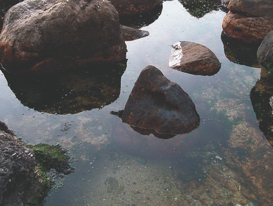
Water, in its liquid form, is either calm or turbulent. When calm, large bodies of water exposed to an intense light source are very reflective. For example, in Figure 11.22 a calm tide pool reflects the sky. Where the water is fairly shallow and is at a perpendicular angle to the viewer, however, the underlying rocks and sand can be seen. This effect is known as a Fresnel reflection and is a result of light moving between two mediums (air and water) with two different refractive indices. (For more information on refractive indices, see Chapter 7.) As such, transparency decreases and reflectivity increases with the viewing angle (the angle between the incoming light ray and the corresponding ray reflected toward the viewer). In addition, the objects underneath the surface are darker than normal since the light received is reduced by sediment within the water.
In Maya, you can use the Sampler Info utility to determine the angle of a water surface to the camera. A simpler solution, however, involves the application of Ramp textures. For example, in Figure 11.23 a primitive NURBS plane replicates calm water. The outAlpha of a ramp texture (named RampReflectivity) is connected to the reflectivity of a blinn material node (named CalmWater). The outColor of a second ramp texture (named RampTransparency) is connected to the transparency of CalmWater. Since the ramps contain only black and white handles, the reflectivity is the strongest at the top of the plane and the transparency is strongest at the bottom of the plane. The camera's Background Color attribute provides the sky color. The scene works with either the Maya Software or mental ray renderer.

Figure 11.23. Two Ramp textures control the transparency and reflectivity of a NURBS surface. This scene is included on the CD as calm_water.ma.
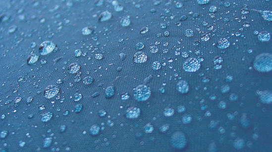
Individual water droplets, a minute form of calm water, reveal a strong tendency to refract. For example, in Figure 11.24 the weave of the cloth is magnified by each drop. The degree of refraction is defined by a refractive index. Although air has a refractive index slightly above 1.0, water has a refractive index of 1.33. When the water's surface is curved by surface tension, the perceived refraction is stronger than the equivalent refraction provided by a flat surface. The surface curvature acts as a convex lens, causing light rays reflected off the cloth to diverge as they are refracted through the water toward the viewer. In addition, the refraction process creates "hot spots" within the drops. These spots are found in caustic regions. Caustic regions are areas in which light rays are focused by materials such as water or glass. In other words, light rays entering the water drop converge toward a focal point.
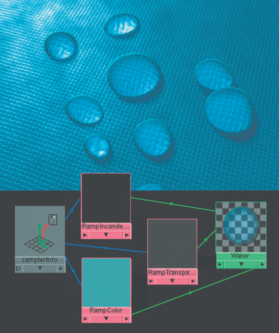
Although the mental ray Caustics attribute is able to produce caustics (see Chapter 12), Maya Software is not. Nevertheless, you can simulate caustics by mapping the material's Incandescence attribute. For example, in Figure 11.25 each water drop is constructed from a NURBS half sphere, which is assigned to a blinn material node (named Water). The outColor of a ramp texture node (named RampIncandescence) is connected to the incandescence of Water. The facingRatio of a samplerInfo utility node is connected to the vCoord of RampIncandescence. The ramp transitions from black to dark blue. Because the center of each drop faces the camera, it receives the dark blue from the top of the ramp, which equates to a slight incandescent glow. The Refractions attribute of Water is also checked and the Refractive Index attribute is set to 3. Although a value of 3 does not correspond directly to real-world water, it produces a satisfactory look. In addition, the facingRatio of the samplerInfo node is connected to the vCoord's two additional ramps (RampColor and RampTransparency). The outColor of RampColor is connected to the color of Water, thus changing the drop color along its edge. The outColor of RampTransparency is connected to the transparency of Water, thus making the drops more transparent in the center.
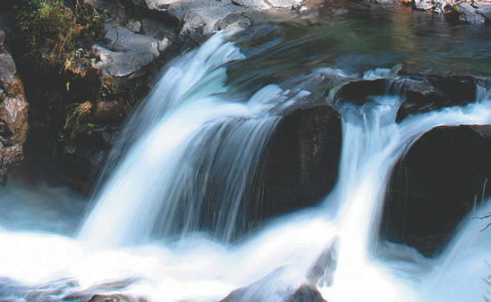
Water that tumbles, crashes, or boils creates a great deal of foam. Foam is composed of numerous bubbles. The white quality of foam (assuming the water is relatively clean) is generated by specular highlights appearing on all the bubbles. For example, in Figure 11.26 a wave hitting a rock appears very white. Yet when a small portion of the water is examined, it becomes clear that the white is composed of numerous specular "hot spots" on countless individual bubbles. Although these spots are actually reflections of a bright sky, they are too small and too dispersed to form a reflection that is coherent. By comparison, calm water produces a single large specular highlight in the form of a large, continuous reflection.

The white quality of foam is often exaggerated by rapidly moving water or a lengthy shutter speed of a still camera. If the water is exposed for 1 second, for example, the water has a chance to move a significant distance and thereby create a strong motion blur. For example, in Figure 11.27 the exposure of a waterfall is long enough to allow the foam to blur into monolithic sheets.
Maya's Fluid Effects system is designed to create turbulent lakes and oceans and comes equipped with foam attributes. If the Maya Ocean system is unavailable, bump and displacement mapping on NURBS or polygon surfaces can emulate the look of foam to some degree. On the other hand, Cloud particles, once flowing through a dynamic simulation, can re-create fast-flowing water. For example, in Figure 11.28 a volume particle emitter generates 3,000 particles per second. The Particle Render Type is set to Cloud and the Radius is set to 0.25. Gravity and Turbulence fields pull the particles downward and randomize their direction respectively. The particles are rendered with mental ray. The Motion Blur attribute is set to Full (No Deformation motion blur is unable to blur software-rendered particles). The length of each particle's blue is exaggerated by setting Motion Blur By to 10. Time Samples is set to 10 to help smooth the result.

When water freezes, it gains new, distinct qualities. For instance, ice cubes, icicles, and other water that is rapidly frozen contain numerous imperfections throughout their mass. Trapped air bubbles, small cracks, boundaries in the crystalline structure, and particulate matter interfere with refractions and reflections. In addition, the convoluted internal structure creates numerous, tiny specular highlights. The end result is a familiar white roughness (see Figure 11.29). The white of the specular highlight is derived from a bright sky or intense camera flash.
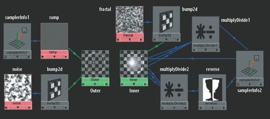
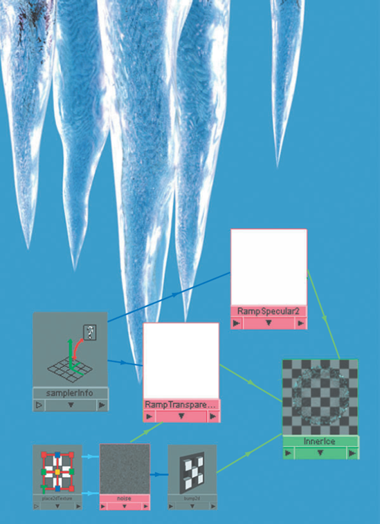
You can reproduce the white specular quality of ice in Maya with Water, Noise, and Ramp textures. For example, in Figure 11.30 icicles are re-created with primitive cones hung upside down. Each icicle is composed of an inner and an outer surface. The outer surfaces are assigned to a blinn material node named OuterIce. The outColor of two ramp textures are connected to the specularColor and transparency of OuterIce. The facingRatio of a samplerInfo utility node is connected to the vCoord of the ramp that controls OuterIce's transparency. This causes the icicles to be more transparent along their cores. In addition, a water texture node is connected to OuterIce's Bump Mapping attribute via a bump2d utility node. The Bump Depth value is set to 0.5, thereby reducing the regularity of the specular highlights. OuterIce's Refractive Index attribute is set to 1.1, which is less than the 1.3 assigned to real-world ice.

The inner surfaces are assigned to a second blinn material node named InnerIce. Two ramp textures are connected to the specularColor and transparency of InnerIce. The facingRatio of a second samplerInfo node is connected to the vCoord of both ramps. This causes the icicles to be transparent and dark along their cores. In addition, a noise texture node is connected to InnerIce's Bump Mapping attribute via a bump2d utility node. The Bump Depth value is set to 36. The Repeat UV of the noise texture's place2dTexture node is set to 10, 4. This creates the crinkled patterns in the center of each icicle. The outColor of the noise texture is also connected to the colorOffset of the ramp controlling InnerIce's transparency. This "dirties" the ramp and makes the transparency inconsistent. The Refractive Index attribute of InnerIce is set to 1.1, causing background icicles to become distorted behind the foreground icicles. The Light Absorbance attribute of InnerIce is set to 20, thus darkening any resulting refraction. Two directional lights strike the surfaces from each side of the screen, highlighting the edges.
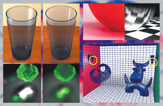
Clear glass is difficult to reproduce simply because there is little to it. Due to its high transparency, glass must be indicated through four main characteristics: reflectivity, refractivity, edge reflectivity, and surface grime.
Clear glass is highly reflective, but not to the point that its transparency is completely obscured. For example, in Figure 11.31 whiskey glasses are photographed in a bright exterior. Several sections of each glass carry intense specular highlight streaks. These streaks are the reflections of the nearby wall and sky. Aside from these washed-out highlights, little else of the surrounding environment is visible in the reflections of the glass. This is due, in part, to the relative brightness of the background wall compared to other parts of the environment. The same glass against a dark background with a strong source of light before it would become more mirror-like (this is similar to the glass of a window or a picture frame viewed at night). Whether the background is bright or dark, a percentage of the light rays striking the glass are absorbed and converted to heat or reflected in such a direction that they do not reach the viewer.

Glass has a refractive index that ranges from 1.45 to 1.85. The distortion of the background by glass objects is fairly subtle unless the glass is thick or the surface is significantly curved, wavy, or faceted. The lips of glasses and vases often appear darker than other parts of the surface. This due to the high degree of curvature present in a small area. In this situation, a percentage of light rays are reflected away from the viewer. In addition, a strong refraction of a dark table or nearby dark wall is often visible (see Figure 11.32). If the glass is in a well-lit location, a light ring is likely to exist just below the dark ring. This ring is generated by the refraction of intense overhead light source.

Along the same lines, the vertical edges of a glass are generally less transparent, and thus more reflective, than the section of the glass facing the viewer. This is another example of a Fresnel reflection, where transparency decreases and reflectivity increases with the viewing angle.
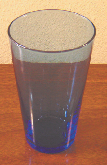
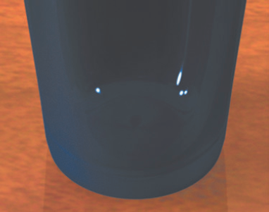
The qualities of clear glass apply equally to colored or tinted glass. For instance, in Figure 11.33 a blue water glass shows reflection, refraction, and a dark top ring.
Last, glass is rarely clean. Fingerprints, dust, and other residue reduce the clarity of the reflections and refractions. The clarity is further reduced by any optical impurities in the glass, such as bubbles or inferior materials.
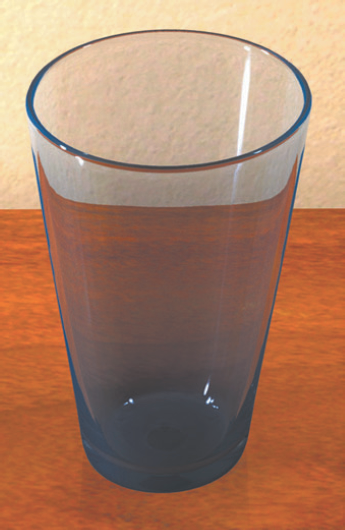
Aside from the reproduction of various glasslike traits, limitations and quirks of the Maya Software renderer pose additional challenges. As an example, the glass pictured in Figure 11.34 is reproduced in 3D.
When comparing the Maya glass to the real glass, you'll see a number of characteristics are equivalent:
The refraction of the table through the glass wall
The vertically stretched specular highlights
The change in transparency from the base to the rim
The characteristic dark, refracted rim
The Maya glass is constructed from a single NURBS surface. (The outline was laid out with a NURBS curve and the Revolve tool applied.) The glass is assigned to an Anisotropic material named GlassColor. The Anisotropic material offers the advantage of elongated specular highlights that can be controlled with additional attributes. The Specular Shading section of the material has the following settings:
Reflected Color is mapped with an Env Cube environment texture. The six walls of the Env Cube are mapped with a photo of the real-world from the "point-of-view" of the glass. That is, photos were taken of what was behind, in front of, beside, below, and above the glass. Since the Reflectivity attribute is set to a low 0.1, the cube provides a subtle hint of the surrounding environment. As for the Raytrace Options section, the following attributes are adjusted:
Refractions: On
Refractive Index: 1.33
Refraction Limit: 10
When you're replicating the refraction of a real-world glass, it is important to match the geometry as closely as possible. If the glass walls are a different thickness or the rim has a slightly different shape, the resulting refraction may be significantly different. For example, in Figure 11.35 the vertices of the NURBS rim are adjusted slightly, producing a refraction that does not match the photo. In fact, if the glass featured in Figure 11.34 were constructed with an even higher degree of accuracy, a more appropriate Refractive Index of 1.45 would work. Ultimately, creating the correct look of a refraction in 3D may require the application of a nonrealistic Refractive Index value.
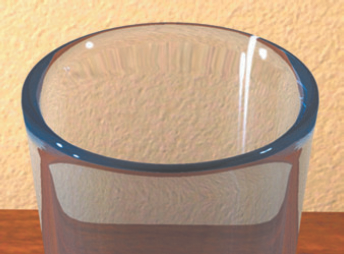
Figure 11.35. When the vertices of the glass surface are adjusted slightly, a significantly different refraction is produced.
Returning to the scene used for Figure 11.34, Light Absorbance is left at the default 0. Although you can raise the Light Absorbance value to darken the glass, the darkening occurs equally over the surface. In this re-creation, the Transparency attribute is instead mapped with a Ramp texture, allowing the base of the glass to appear darker. The Ramp itself has four handles that create a white band in the center of a gray field. This forces the base to be more opaque and the rim more transparent.
Last, the Maya Software renderer has the following settings:
Shading: 2
Max Shading: 10
Reflections: 10
Refractions: 10
Shadows: 2
If Refractions is not set to the maximum value, some parts of the glass turn into "black pits." For example, in Figure 11.36 Refractions is set to 2. The base of the glass becomes solid black because the refraction rays are killed off before they have a chance to intersect all the walls of the glass and reach the table top. The color black is provided by the Background Color of the rendering camera. In Maya, Background Color is the color of empty space.
In some cases, black pits are much more subtle. Even when Refractions is set to 10, they can occur with intricate geometry or with surfaces that possess complex angles. In fact, you can see black pits in the upper-left corner of the icicle render in Figure 11.30. In a separate example, a clear glass produces small black pits at its base (see Figure 11.37). The quickest solution is to change the Background Color to something other than black. With Figure 11.37, a brown Background Color helps solve the problem.

When you compare the Maya glass featured in Figure 11.34 to the real glass in Figure 11.33, you'll see that several characteristics are not equivalent:
The refraction is much smoother on the Maya glass. The refraction of the real glass is slightly wavy due to the variations in the thickness of the glass wall.
Most important, the Maya glass is missing the hot blue caustics spots at the base. These can be created with the mental ray Dielectric_material shader, which is demonstrated in Chapter 12.
In this tutorial, you will texture and render an ice cube with the mental ray renderer. You will employ reflections, refractions, and custom shading networks to help make the render more realistic (see Figure 11.38).
Open
icecube.mafrom the Chapter 11 scene folder on the CD.Create two new Blinn materials in the Hypershade window. Name the first Blinn material Inner and the second Blinn material Outer. Assign Outer to the OuterIce polygon surface. Assign Inner to the InnerIce polygon surface.
MMB-drag Outer into the work area and open its Attribute Editor tab. Set Transparency to 100% white, Eccentricity to 0.1, and Specular Color to 100% white. Check the Refractions attribute. Set Refractive Index to 1.4 and Refraction Limit to 2.
Click the Bump Mapping attribute Map button. Choose a Noise texture from the Create Render Node window. Open the Attribute Editor tab for the new bump2d node. Set the Bump Depth attribute to 0.1.
MMB-drag a Ramp texture and a Sampler Info utility from the Create Maya Nodes menu into the work area. Connect the facingRatio of the samplerInfo node to the vCoord of the ramp node. Connect the outColor of the ramp node to incandescence of Outer. Use Figure 11.39 as a reference.
Open the ramp node's Attribute Editor tab. Change the Interpolation attribute to Smooth. Delete the middle color handle. Change the top color handle to dark gray. Change the bottom handle to medium gray. Position the top handle two-thirds of the way up the ramp. This ramp will control the bright edge of the ice cube. If the cube edges render too brightly, darken the colors of this ramp. The Outer material is now complete.
MMB-drag Inner into the work area and open its Attribute Editor tab. Click the Bump Mapping attribute Map button. Choose a Fractal texture from the Create Render Node window. Open the Attribute Editor tab for the new bump2d node. Set the Bump Depth attribute to 0.2.
MMB-drag a Sampler Info, a Reverse, and two Multiply Divide utilities from the Create Maya Nodes menu into the work area. Connect the facingRatio of the samplerInfo node to the inputX of the reverse node. Connect the facingRatio of the samplerInfo node to the specularRollOff of Inner. Connect the facingRatio of the samplerInfo node to the input1X of the multiplyDivide1 node. Connect the outputX of the multiplyDivide1 to the incandescenceR, incandescenceG, and incandescenceB of Inner. Connect the outputX of the reverse node to the input1X of the multiplyDivide2 node. Connect the outputX of the multiplyDivide2 node to the transparencyR, transparencyG, and transparencyB of Inner.
Open the Attribute Editor tab for multiplyDivide1. Set the Input2X attribute to 0.3. Increasing this value will create a stronger "glow" around the ice cube's edge.
Open the Attribute Editor tab for multiplyDivide2. Set the Input2X attribute to 2.75. Decreasing this value will make the edges of the ice cube cloudier and less transparent. The custom shading networks are now complete!
The scene file contains a single directional light named Key. Open the Attribute Editor tab for Key and check Use Ray Trace Shadows. Set Light Angle and Shadow Rays to 5. This creates a soft-edged shadow. Set Ray Depth Limit to 5. This limits shadows to four recursive reflections or refractions.
Open the Render Settings window. Switch the Render Using attribute to mental ray. Set the Quality Presets attribute to Draft. Render out a test. If it looks good, switch Quality Presets to Production and rerender. The tutorial is complete! If you get stuck, a finished version is included as
icecube_complete.main the Chapter 11 scene folder on the CD.