
Chapter 11
Beyond “Point and Click” with JMP
Thus far we have emphasized that Visual Six Sigma projects, because they are focused on discovery, necessarily involve working with data interactively to uncover and model relationships. The case histories in the preceding six chapters illustrate how JMP can support this pattern of use better than most other software.
However, as a project nears completion in the Utilize Knowledge step, there is a need to preserve and perpetuate the resulting performance gains. This usually requires monitoring the process over time. In turn, this leads to the broader question of how we can automate an analysis so it will work with new data with minimal effort from us. Here we use the word automate in the general sense of saving our collective effort and time, rather than in any technical sense (an example of the latter is the COM standard from Microsoft for interoperation of software components, which JMP also supports).1
This chapter provides a brief discussion of automation. This topic is of importance not just for Visual Six Sigma but also for the effective and efficient use of JMP in more general contexts. In Chapter 3 we touched on a related, even overlapping, topic when we reviewed how to personalize JMP to make it better fit the skills and requirements of a user or group of users. Generally, appropriate personalization saves time and effort, sometimes to the point of making an analysis viable when it otherwise would not be.
So this chapter is a discussion of how JMP supports more automated and personalized usage patterns that go beyond the informed “pointing and clicking” that lies at the heart of discovery. This is a big topic, so to keep the discussion manageable, we anchor it in a specific example and then conclude with a summary containing some specific recommendations for further study. We start with a few comments about the science and art of programming and of building applications designed to do specific things.
The data sets used in this chapter are available at http://support.sas.com/visualsixsigma and can be accessed using the journal, Visual Six Sigma.jrn.
PROGRAMMING AND APPLICATION BUILDING IN JMP
Given that our intention is simply to convey general ideas, we can afford to be a little lax in terminology. With this in mind, we define an application as something added to the core product (in this case JMP) that does something that is considered useful.
Generally, an application, A, has three parts:
- Part A1: A user interface, to gather inputs from a user each time it is run
- Part A2: Some processing logic
- Part A3: A report containing the results
The application usually also contains aspects of automation and of personalization. Application building often requires a programming or coding effort from specialists, and different software environments can make this activity easy or hard.
Depending on the scope and intended purpose of the application, Part A1 is sometimes not needed because the inputs do not change. Part A3 is always needed if we interpret the report as the means of conveying results either to the user or to some other processing system.
In Chapter 3 we introduced the idea of scripts using the JMP Scripting Language (JSL). We repeatedly used saved scripts to expedite and reproduce analysis steps in the subsequent chapters.
Although coming to terms with a new programming language can be an interesting and rewarding intellectual exercise, building useful applications in JMP often does not require such a commitment. This is because, as you point and click in JMP, JMP automatically generates JSL that can regenerate the state of the report with which you are working. This code can be saved for reuse. For simple applications, this code forms the basis, sometimes the entirety, of Part A2 above.
As pointed out in Chapter 3, if you save a script to the data table that generates a report, you can easily reproduce the analysis in question even if you change the rows in the table (by adding or deleting rows, or changing the contents of cells) or if you add columns to the table (which the saved script ignores). However, if you delete a column that is needed by the script, then the script will fail and it will write an appropriate message to the JMP log window.
The fact that JMP generates code for you is a great time-saver and also means that the barrier to understanding and becoming proficient in JSL is considerably reduced should you wish to dig deeper. However, whatever your attitude toward programming, you might want to become familiar with the basics of how to write JSL by hand and the facilities that JMP offers in support of writing JSL. So before moving on to our main example, we consider how to approach the traditional “Hello World!” example in JSL.
To write a new script, select File > New > Script to open an empty editor window. Right-click in the editor window and select Show Embedded Log from the context menu. The window is split and any messages generated by your code will appear in the lower pane of the window. (Alternatively, you can open a separate log window using View > Log.)
Type (or copy and paste) the following on a single line in the upper pane of the editor window:
For(counter = 1, counter <= 5, counter++, Print(“Hello World “||Char(counter)||”!”) );To run the code, select Edit > Run Script or right-click in the script window and select Run Script from the context menu. The code produces Exhibit 11.1. (This code is contained in the script Hello World!)

Exhibit 11.1 JSL Script and Output
You have successfully built your first working application by hand. Here is a little background on how it works:
- The numeric variable
counterstarts with the value 1 and is incremented in steps of 1 to the value of 5 by theFor()loop. Note that the expressioncounter++is an abbreviation forcounter = counter+ 1. -
The
For()function contains four arguments that are separated by commas:- The initial argument (
counter = 1) - The while argument (
counter <= 5) - The next argument (
counter++) that controls iteration - The body argument (the
Print()command)
The
For()function is a typical looping construct found in programming languages. It repeatedly executes the body argument (in this casePrint()) so long as the while argument (counter <= 5) remains true. - The initial argument (
- As you might expect,
Print()echoes its arguments to the JMP log, one per line. In this case, there is only one argument, made up of three pieces of text concatenated together using the symbol || (alternatively written asConcat()). To obtain the number in text format, we have to convert the numeric value ofcounterto a character format. This is done usingChar().
Like every language, JSL has its own syntax rules. We do not attempt to treat these in detail, but refer you instead to Help > Books > Scripting Guide for all the details if you need them. If your code does not satisfy these rules, an appropriate error message is sent to the log. This message should help you to diagnose the failure. A few general comments may help, though:
- Generally speaking, JSL is case-insensitive and ignores embedded white-space.
- As with every language, brackets, parentheses and braces have to balance.
- JSL expressions are glued together with a semicolon (;). The trailing ; at the end of the only line in our “
Hello World!” example is not required because there is no following expression. - On your computer screen, the code that you type will be color-coded. Keywords are shown in blue, literal text in purple, and comments in green.
- The editor provides autocompletion, so if you type the first part of a keyword and press
Control-Spaceon Windows (Option-Escon Macintosh), you will be given a list of keywords that match what you have typed so far. - If you hover the mouse over a keyword, the editor displays a tooltip showing short help on the syntax and arguments that keyword requires.
- Scripts can be saved to files with a .jsl extension (and restored from such files) using
File > Save AsandFile > Open, respectively.
If you are writing more extensive code, you may need some of the options that are available in the Edit menu or with a right-click in the script window. The Reformat Script option reformats your code to make it easier to read. By turning on a Script Editor preference (File > Preferences), you can also use code folding to hide blocks of code to improve readability.
A MOTIVATING EXAMPLE: DEMOCRACY AND TRADE POLICY
This example shows the steps in building an application to study missing data, and relates to Chapter 4, since missing data is a key aspect of data quality. As you will see, the application extends the functionality offered in earlier versions of JMP, although some of this is now provided in the core product itself. We first walk through the manual steps to produce the required analysis and then introduce an application that accomplishes the same thing. We then briefly review the new, related functionality in JMP. Finally, we dissect the application to get an insight into how it works.
Understanding the pattern of missing data can give you important clues about the data-generating or data-recording processes. These clues can help you avoid the occurrence of missing values in the future. For some problems you may be forced to guess (or impute) values for missing cells just to make a subsequent analysis more viable or informative. This is done through a numerical process called imputation. Of course, any imputation technique makes assumptions that you need to check. Specifically, most imputation techniques rely on the assumption that the values of variables are missing at random, which may or may not hold.2
The Free Trade Data
For simplicity of illustration and discussion, we will use a small example consisting of only ten variables. But the power of the principles and techniques you will see are equally relevant and even more valuable in situations where you have a large number of variables, especially if your focus is on prediction.
This example shows you how to conduct a deeper analysis of missing values. The data address the effect of democracy on the trade policy of nine developing countries (or polities) in Asia from 1980 to 1999.3 The table Freetrade.jmp, shown in Exhibit 11.2, includes ten variables: year (year), country (country), average tariff rates (tariff), Polity IV score4 (polity), total population (pop), gross domestic product per capita (gdp.pc), gross international reserves (intresmi), a dummy variable signifying whether the country had signed an IMF agreement in that year (signed), a measure of financial openness (fiveop), and a measure of U.S. hegemony (usheg).

Exhibit 11.2 Table Freetrade.jmp (Partial View)
Open the data table Freetrade.jmp. Select Tables > Missing Data Pattern, select all the columns, click Add Columns, and then click OK. This gives the new table Missing Data Pattern shown in Exhibit 11.3. (Running the saved script Missing Data Pattern in Freetrade.jmp generates the same table.)

Exhibit 11.3 Table Missing Data Pattern (Partial View)
The Missing Data Pattern data table contains three scripts. Selecting Run Script from the red triangle menu for either the Treemap or Cell Plot script gives a visual representation of the missing data.
Although very useful, Missing Data Pattern may not directly contain all the information you need. For example, suppose that you want to see the number of rows where a given number of columns are missing. Using the Missing Data Pattern table, you need to select Tables > Summary, select Count and then select Statistics > Sum, assign Number of Columns Missing to the Group role, and click OK. Similarly, if you want to rank the columns in order of missingness, you need to use the Cols > Column Viewer menu option with the table Freetrade.jmp active, then make an auxiliary table and sort it appropriately.
To further investigate the pattern of missing data, we will use two complementary techniques to see how the columns group together: Principal Components Analysis (PCA) and Clustering. The first technique can be conducted directly from the Missing Data Pattern table, but the second requires some additional manipulations.
Principal Components Analysis
PCA exploits correlations among variables to produce a data description that is more concise, in the sense that it requires fewer dimensions. In so doing, it can also show which, if any, variables group together to achieve this reduction.4 Your hope is that PCA will help you better understand how your missing values are structured.
Because you are interested in how missing values occur across your variables, rows with no missing values contain no useful information. So you begin by excluding the row in the Missing Data Pattern table that represents no missing values. Then you conduct a principal components analysis on the Missing Data Pattern table. (There is a copy of the Missing Data Pattern table, with scripts that reproduce the work in this section, in the journal file. But this table is not linked to Freetrade.jmp.)
Ensure that Missing Data Pattern is your active data table, select the first row, and select Rows > Hide and Exclude. Because the Missing Data Pattern table that you created and the Freetrade.jmp tables are linked, this also hides and excludes the corresponding rows in Freetrade.jmp. (Keep in mind that the Missing Data Pattern table from the journal is not linked to Freetrade.jmp.)
Now select Analyze > Multivariate Methods > Principal Components. Note that Count was automatically assigned to the Freq (Frequency) role in the Missing Data Pattern table. (A column can be assigned the Freq role by right-clicking it in the Columns panel and selecting Preselect Role > Freq.) Enter your original variables, year through usheg, as Y, Columns (see Exhibit 11.4).

Exhibit 11.4 Principal Components Launch Dialog
Click OK. Click Continue when a JMP Alert warns you that columns are not Continuous. Click OK when a JMP Alert warns you that five columns are being dropped because they are constant. The report appears as shown in Exhibit 11.5.

Exhibit 11.5 Principal Components Report for Missing Data Pattern
Keep in mind that, in this analysis, we are not analyzing the data themselves, but the nominal columns that indicate whether a cell is missing. These are the nominal columns marked by the red icons in the Columns panel of Missing Data Pattern.
The plot on the right in Exhibit 11.5 is called a loadings plot. It represents how the indicator variables appear in the reduced two-dimensional space. Note that the plot shows only five points, since five other variables are omitted because they are constant.
The Pareto plot on the left of this figure indicates the amount of variation explained by each eigenvalue. The first two eigenvalues, which define the first two dimensions or principal components, account for about 71 percent of the variability between the indicator variables. The rest of the variability is spread among the higher components. For other data, though, the two first components may not capture enough variability, in which case the alignment and lengths of the arrows in the loadings plot would not be so helpful in seeing which columns group together.
For these data the loadings plot shows, with some credibility, that intresmi, a measure of gross international reserves, groups with fiveop, a measure of financial openness in terms of missing values. As an exercise, see if you can verify that fiveop is missing for the years 1998 and 1999 and that intresmi is missing for all nine countries in 1999, but only missing for four countries in 1998. (In Freetrade.jmp, select the columns intresmi and fiveop. Use the column modeling utility Cols > Modeling Utilities > Explore Missing Values to select the rows where intresmi and fiveop are missing. Then use Tables > Subset.) Given that 1998 and 1999 were the final years for this study, is it possible that the two measures in question either were not available yet, or were just beginning to be available?
Cluster Analysis
As mentioned previously, clustering of variables5 is a complementary technique to PCA for grouping variables together. However, it requires some additional manipulations because the entities to be clustered have to appear as rows in a data table. Your Missing Data Pattern table contains an indicator column for each variable that you could transpose. But you also need the information in the Count column. This information would be lost if you simply transposed the columns in the Missing Data Pattern table.
So you need to return to the table Freetrade.jmp to make some progress. Close Missing Data Pattern without saving it.
As you did for the PCA, you will drop all rows that have no missing values. If you have followed the steps above (with your own Missing Data Pattern table), then you find that 96 rows in Freetrade.jmp are hidden and excluded, but also selected. If these rows are not excluded, run the script Hide, Exclude, and Select Complete Rows in the Freetrade.jmp data table that you can open from the journal. Use Rows > Row Selection > Invert Row Selection to select all rows that contain one or more missing values. Then select Tables > Subset and click OK to construct a new table called Subset of Freetrade that has 75 rows.
You now have to create the ten indicator columns that were generated automatically for you in Missing Data Pattern. Although you can do this by defining formula columns like the one shown in Figure 11.6, this becomes very tedious when there are many columns. It is more efficient to use a little JSL instead.

Exhibit 11.6 Formula Column for Missing Row Indicator for fiveop
Note that the formula uses the Is Missing() function combined with a conditional If statement to indicate missing values of fiveop with a 1 and nonmissing values with a 0. Your script will use this structure.
Select File > New > Script to open a script editor window, and then type in the lines shown in Exhibit 11.7. (This script is Make Indicator Columns.jsl, found in the journal.)

Exhibit 11.7 Rudimentary JSL for Table of Indicator Columns
Select Edit > Run Script to produce a new table with the same number of rows and columns as the original, but containing the appropriate pattern of zeroes and ones. The code works as follows:
- Line 1 saves a reference to the currently active data table (
Subset of Freetrade) asdt. - Line 2 tells JMP to place all columns in
dtinto the matrixm. - Line 3 replaces entries in
mthat are not missing by 0. - Line 4 replaces entries in
mthat are missing by 1. - Line 5 constructs a new data table from the matrix
m.
The Is Missing() function returns the value 1 if a value is missing and value 0 otherwise. The exclamation point in Line 3 (!Is Missing()) indicates that a value is not missing. The Loc() function finds all positions in a matrix where a logical condition is satisfied. You can run the lines one by one (select each in the editor window, then Edit > Run Script) and view their effect in the log window.
The new table will be called Untitled X where the value of X is determined by what else you have done in your current JMP session. Note also that, although the columns are in one-to-one correspondence with those in Freetrade.jmp and Subset of Freetrade, the new column names are generic (Col1, Col2, and so on). You can retain the original column names by using the slightly more complicated script shown in Exhibit 11.8 and listed as Make Indicator Columns 2.jsl in the journal. Lines 2 and 7 give the new table a better name, and line 6 (corresponding to line 5 in Make Indicator Columns.jsl) is modified to ensure that the column names are those in the original table.

Exhibit 11.8 More Useful JSL for Table of Indicator Columns
Close Untitled X without saving it. Run the new script using Edit > Run Script to produce the table Subset of Freetrade Missing Cells shown in Exhibit 11.9. (You can also open this data table by clicking on the link for Subset of Freetrade Missing Cells.jmp in the journal file.)

Exhibit 11.9 Table Subset of Freetrade Missing Cells (Partial View)
Now you need to rearrange the data so that each variable occupies a row. Select Tables > Transpose. Add all columns to the Transpose Columns list. Enter For Clustering as the Output table name and Variable as the Label column name. (See Exhibit 11.10.) Click OK to produce the table For Clustering. This table should have 10 rows and 76 columns.

Exhibit 11.10 Completed Transpose Dialog for Subset of Freetrade Missing Cells
Now your data are in the appropriate form for the cluster analysis. Select Analyze > Multivariate Methods > Cluster. Add Row 1 through Row 75 as Y, Columns. To select all 75 rows easily, click Row 1, scroll to Row 75, then press the Shift key, and click Row 75. In the Method panel, select Fast Ward. (See Exhibit 11.11.) Click OK. (We use the Fast Ward method for efficiency in clustering other data with a large number of rows.)

Exhibit 11.11 Completed Cluster Dialog for For Clustering
In the report that appears, the rows in For Clustering (columns in Subset of Freetrade) have been grouped together as shown in the tree-like plot, called a dendrogram. Select Color Clusters and then Mark Clusters from the red triangle menu.
Note that the dendrogram is interactive, and that you can drag the diamond-shaped hotspot to change the number of clusters that you want to consider. In Exhibit 11.12 we have chosen three clusters. The variables year, country, pop, gdp.pc, usheg, polity, and signed form one cluster. These are the variables that are either never or rarely missing. The variables intresmi and fiveop form a second cluster, and tariff forms a singleton cluster.

Exhibit 11.12 Cluster Report for For Clustering
Remember that the three clusters relate to missing values for these variables, and not to their actual values. In other words, the clusters group variables that are similar in terms of which values could not be obtained, for some reason. Recall that the PCA analysis also indicated that intresmi and fiveop had some commonality in terms of missing values.
This analysis of missing values beyond that provided by Tables > Missing Data Pattern can provide additional insight. As we mentioned earlier, it is likely to be more useful when your data contain many more columns than Freetrade.jmp. If you analyze large observational data sets frequently, you might like to automate the manual process you just performed. Fortunately, it is relatively easy to automate all of the preceding steps using JSL, particularly since, as we mentioned earlier, JMP itself will generate most of the JSL code required. In a sense, you simply string the code together to form an application.
The Missing Data Add-In
When developing applications, an important question to consider is how they can be deployed and updated in a simple and foolproof way. As well as making the application development easy, JMP also eases deployment issues through an “add-in” architecture. An application can be packaged up into a single .jmpadin file that can be given to each user who needs it; the user can install it with a single click.6
The file Missing Data.jmpaddin is a JMP add-in that contains the application that automates the above steps. Click on Missing Data.jmpaddin in the journal file. A JMP Alert asks if you would like to install the add-in. Click Install. This creates a new Add-Ins menu in the JMP toolbar and installs a Missing Data submenu in that menu. If you already have an Add-Ins menu, the new item will just be appended.
Making sure that Freetrade.jmp is the active data table, and that no rows are excluded, select Add-Ins > Missing Data > Missing Analysis to produce Exhibit 11.13. The report created by the add-in combines the results in Exhibit 11.5 and 11.12 into a single report, and also includes Pareto charts for missingness by row and by column. In the report generated by the add-in, note that menus are active and plots are interactive.

Exhibit 11.13 Missing Analysis for Freetrade.jmp Using the Add-In
The Missing Data add-in contains other options:
Missing Data > Demo Datagenerates another copy ofFreetrade.jmp.Missing Data > Missing Mapshows the arrangement of missing values in the table in the form of a cell plot.Missing Data > Impute Using Ameliaprovides an advanced way to impute data values using the R package Amelia,7 and requires R to be installed locally.8
As well as showing some further useful analysis of missingness, this analysis of Freetrade.jmp illustrates a number of points:
- A method for addressing a specific data issue interactively
- An insight into the utility of JSL to assist such one-time data tasks
- A view of the value of add-ins when you need to routinely supplement existing JMP functionality and make this available to others
JMP 12 Functionality for Missing Data
However, JMP itself now offers much of this functionality directly, greatly speeding up and simplifying the workflow for handling missing data.
Make Freetrade.jmp your active table and select all the Continuous columns in the data table. Then select Cols > Modeling Utilities > Explore Missing Values. This generates the report shown in Exhibit 11.14.

Exhibit 11.14 Explore Missing Values for Continuous Columns in Freetrade.jmp
The view in Exhibit 11.14 is for the Missing Value Report option. There are four other options:
Missing Value Clusteringprovides clustering similar to that described above, but directly.Missing Value Snapshotshows the cell plot given by the Missing Map option provided by the add-in.Multivariate Normal Imputationimputes missing values of continuous values under the assumption of multivariate normality, but also allows you to shrink the estimated covariance matrix, which can provide more reliable values. Note that this option updates the source data table, highlighting cells containing imputed values in light blue. This option should provide somewhat similar imputed estimates to the add-in that uses the Amelia package, but does not require a local R installation.Multivariate SVD Imputationprovides an efficient computational approach for imputation for data tables with a large number (hundreds or thousands) of variables.
Note that JMP and JMP Pro also provide other ways to handle missing data, depending on the objectives of the subsequent analysis:
Analyze > Multivariate Methods > Multivariateallows you to impute missing values from a set of continuous variables. LikeMultivariate Normal Imputation, it assumes that the variables follow a multivariate normal distribution. UseImpute Missing DataorSave Imputed Formulafrom theMultivariatered triangle. Note that this option does not provide shrinkage estimates.- For predictive modeling,
Analyze > Fit Model,Analyze > Modeling > Partition, andAnalyze > Modeling > Neuralall provide an informative missing approach. For a continuous column, this option replaces missing values with the mean of the nonmissing values and adds an indicator column for the missing values. Both columns are included in the modeling process. By using the informative missing option, you avoid the problem of decimating your data through deletion of rows with one or more missing values. This process usually produces models with better predictive ability.
Finally, note that JMP also provides utilities to explore outliers. Select the columns of interest in the data table and then select Cols > Modeling Utilities > Explore Outliers. Exploring outliers is often of great value in the early phases of handing real-world data.
BUILDING THE MISSING DATA APPLICATION
In this section we give some insight into how the missing data application was built. The discussion is at a high level, but the source code is provided if you want to dig deeper to understand more of the details.
The Structure of the Add-In
As you have seen, the Missing Data.jmpaddin creates an Add-In submenu, Missing Data, that has the four suboptions shown in Exhibit 11.15. Each option invokes the code in the single JSL file whose name is shown in the table.
Exhibit 11.15 Missing Data Add-In: Options and Scripts
| Menu Item | JSL File Name |
| Demo Data | makeDemoData.jsl |
| Missing Map | missingMap.jsl |
| Missing Analysis | missingDataAnalysis.jsl |
| Impute Using Amelia | multipleImputationWithAmelia.jsl |
The script makeDemoData.jsl, found in the journal, only contains the commands required to make a new copy of the table Freetrade.jmp. This script was generated by using the Copy Table Script option from the red triangle of the table, pasting the results into an editor window, and saving the file with the required name.
Using the Missing Map option when Freetrade.jmp is active produces Exhibit 11.16.

Exhibit 11.16 Missing Map of Freetrade.jmp (No Columns Selected)
The list shows all the columns in the data table with missing values, but ranked in descending order in terms of how many values in that column are missing. Selecting the first three columns in the list gives Exhibit 11.17, with the positions of missing cells shown in red. Moving the sliders allows you to change the size of the plotted cells.

Exhibit 11.17 Missing Map of Freetrade.jmp (First Three Columns Selected)
The JSL Code for the Missing Data Add-In
The script Missing Data.jmpaddin contains all of the elements of an application (Parts A1, A2, and A3) listed earlier. The section of code that creates the window shown in Exhibit 11.16 is shown in Exhibit 11.18. You can see that the user interface is built up from a number of components or objects (display boxes) such as TextBox(), ButtonBox(), and SliderBox() with names describing what they do. As mentioned earlier, you can use the editor tooltips to learn more about these objects. Alternatively, you can use Help > Scripting Index to search for the object you require. The Scripting Index describes the object and provides one or more examples of how that object can be used. You can run these examples and experiment with them.

Exhibit 11.18 JSL Code to Produce Exhibit 11.16
The display boxes in the script in Exhibit 11.18 are laid out according to the other display boxes that appear at higher levels in the code (PanelBox(), HListBox(), LineUpBox(), SpacerBox(), and VListBox()).
Each object understands a set of messages that influence its behavior. For example, the SetWrap() and FontColor() messages are sent to the first TextBox() using the JSL “≪” operator. Each object can optionally be given a name so that it can be referenced in other parts of your code (for example, clb = ColumnListBox()).
The user interface updates when you interact with the ListBox(), ButtonBox(), or SliderBox() objects. The action that occurs is determined by the JSL expression associated with the object. For example, the expression clbChangeScript is associated with clb. The code in clbChangeScript is shown in Exhibit 11.19.

Exhibit 11.19 Code that Runs When ListBox() clb Updates
Note the following:
- To define a JSL expression, you use the syntax
variable = Expr(expression)where the required statements are insideExpr(). This postpones the evaluation of these statements until the action is needed. In this case, the action is postponed until the selection inclbis changed by the user. - Line 72 puts the names of the selected items in
clbinto a list calledsc(by sending the messageGetSelected). - Line 73 calculates
ncs, the number of items in the listsc. - Line 74 invokes the expression
gbUpdateScript, which uses the information now in the listscand the variablencs. This expression adds or updates aGraphBox(). This is the cell plot that is seen in Exhibit 11.17.
Application Builder
Rather than write the code for the user interface, Part A1, by hand, an alternative approach, preferable for most people, is to use the Application Builder in JMP. As the name implies, the Application Builder is a design-time tool that allows you to build user interfaces simply by “drag and drop,” rather than by coding by hand. You can also add the required processing logic, Part A2, to each object in your application, producing modularized and maintainable code with minimal effort.
Select File > New > Application to open the Application Builder window. This window consists of three parts:
- On the left is a list of all the objects that you can put into an application, arranged into major groupings by outline nodes (
Reports,Data Table,Containers, and so on). - In the middle is the canvas, initially blank, on which you will design your application by dragging the required objects from the left.
- On the right are the
ObjectsandPropertiesoutlines. TheObjectspanel gives an alternative, tree-based view of your application, and thePropertiespanel allows you to modify the properties of the object currently selected on the canvas. By unchecking the red triangle optionShow Objects and Properties, you can make the canvas bigger if you need to.
The first display box needed is a PanelBox(), found in the Containers outline. Exhibit 11.20 shows the Application Builder after you have dragged this component onto the canvas and updated its properties. In this case, the only property is the text that is displayed as a title.

Exhibit 11.20 Starting to Build Your User Interface with a PanelBox()
By dragging the required components into the template and modifying their properties appropriately, you can construct the canvas shown in Exhibit 11.21. You can compare the code in Exhibit 11.18 to Exhibit 11.16 to help figure out which components are needed from the palette and what their relationship should be. (Alternatively, simply open the file missingDataUI.jmpappsource.)

Exhibit 11.21 Missing Data User Interface in Application Builder
To view the final user interface, select Run Application from the red triangle menu in Application Builder. This produces the window shown in Exhibit 11.22. Compare this with Exhibit 11.16.

Exhibit 11.22 Missing Data User Interface from Application Builder
Application Builder is a capable and complete platform. If you need additional help to develop applications, we encourage you to look at the relevant documentation (Help > Books > Scripting Guide). Finally, we note in passing that the very useful Window > Combine Windows feature mentioned in Chapter 3 (for combining several report windows into one) actually builds an application, which you can further modify with Application Builder if you wish to.
Interoperability with R
Finally, we turn to the last menu item in the Missing Data add-in, Impute Using Amelia. If you open the associated code in multipleImputationWithAmelia.jsl and run it with Freetrade.jmp as the active table, you will see that a dialog appears that allows you to select columns and options. Having made some selections, when you click OK you see a message indicating that data is being submitted to R. If you do not have R installed, then you receive an error message to that effect. If you do have R installed, along with the Amelia package and all of its dependencies, then a copy of Freetrade.jmp appears with missing cells replaced by imputed values. These cells are colored orange to distinguish them from data that are real.
The code that produces the initial dialog appears in lines 23 to 78 of the script multipleImputationWithAmelia.jsl. You can verify this if you select all the lines from the first down to 78 in the editor window and then Edit > Run Script. Although this interface is more complex than the interface for the Missing Map, the principles are the same, and this code could be generated by Application Builder or written by hand.
The report produced by this script, Part A3, is also simple (just making a new table). So the essentially different feature is the processing logic, Part A2, and the fact that this is not done by JMP, but by another system (in this case R). Even though JMP is incredibly functional, there may be times when you need capabilities that it does not provide. Clearly, using this approach will involve some knowledge of the other system.
To see how JMP can interoperate with R, select Help > Scripting Index, select Functions from the dropdown list, and type “R” in the search box at the upper left (Exhibit 11.23). Select Exact Phrase from the tools menu, which you obtain by clicking the gear icon to the right of the search box. You will see that there are 13 related functions whose names begin with “R”. Essentially we need to be able to connect to an R session (R Init()), and disconnect from an R session (R Term()), to move data both ways across an active connection, to run R code, and to retrieve textual and graphical output from R. The R functions listed handle all these aspects. We will look at some code fragments from multipleImputationWithAmelia.jsl to get a feel for how they are used.

Exhibit 11.23 Functions That Allow JMP to Interoperate with R
Exhibit 11.24 shows the definition of a JSL function (packageInstalled()), and how it is used in the later code. Similar to the add-in framework in JMP, R uses the concepts of packages that can be downloaded from repositories and installed locally. Amelia is one such package. Once we have an active R connection, we need to check that the required package is available. If it is available, we load it (line 162), and if it is not, we present a warning message and stop the execution of the script (line 161).
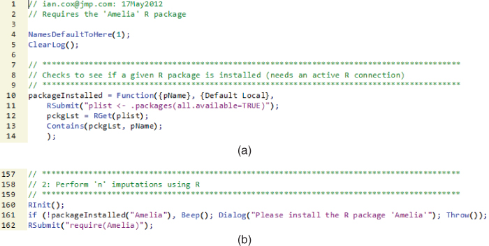
Exhibit 11.24 Loading the R Package Amelia
Lines 10 to 14 show the syntax for defining a function in JSL. The variable pName contains the name of the package we are looking for. Using R Submit(), line 11 runs the R code required to see which packages are available, and puts the results into plist. Line 12 then uses R Get() to move the contents of plist into a JSL variable, also a list, called pckgLst. Line 13 then evaluates to a Boolean value that is returned when packageInstalled() is evaluated (the value 1 if pckgLst contains pName and the value 0 if not). Line 162 loads the Amelia package once we are sure it is available.
Exhibit 11.25 shows how the imputation is performed. Line 163 sends the JMP data table referenced as dt2 to R: R Send() translates a JMP table to an R data frame with the same name. Line 165 builds the R code for using Amelia, and returns the results to the R structure imputation.results. Note that the Amelia package is very functional and provides a lot of control over how the imputation is carried out. Only the simplest options are surfaced in the initial JMP dialog, and this is reflected in the code in line 165. Line 167 then uses RGet() to retrieve the results into a JSL variable, dt2List. This is actually a list of data tables (each containing imputed values). The variable n comes from the initial dialog and is the number of imputations we asked for. If the dialog option Keep Each Imputation is left at the default value of No, dt2List will contain a single table with imputed values equal to the average of the n that were performed. Otherwise, it contains n tables with no averaging of the imputed values.

Exhibit 11.25 Using the R Package Amelia for Imputation
To understand all the details of how the code works, see the comments in the code itself.
The mechanics of packaging code and other resources into an add-in are straightforward (see Help > Books > Scripting Guide). If you are working entirely with the Application Builder, you can simply select Save > Save Script to Add-in from the red triangle menu.
Note that JMP provides the same style of interoperation with MATLAB as it does with R. So, if you have an investment in specialized code in this system, you can make its capabilities available to users who might be intimidated by, or unwilling to learn, that software. If you search for MATLAB in the JSL Scripting Index, you will see JSL functions analogous to those used in the Missing Data application. You can compare the results of your search with Exhibit 11.23.
You should also be aware that JMP can act as a client to SAS, and can interoperate with SAS in many different ways. The built-in client functionality allows point-and-click access to many SAS resources such as stored processes, and as a SAS product it has a depth of integration that is deeper than with other software. If you search for SAS in the JSL Scripting Index, you will find 40 associated JSL functions, which indicates a world of many possibilities.
CONCLUSION
The intention of this chapter was to show some of the possibilities for building useful applications using JMP. In the Visual Six Sigma context, such applications are usually associated with the Utilize Knowledge step when you need to assure that the performance gains are institutionalized. Left alone, any system degrades over time. Appropriate ongoing monitoring is an essential part of this endeavor.
Of course the usefulness of applications extends far beyond the Visual Six Sigma context. If you have made an investment in JMP, it's good to be aware of what is possible. As should now be clear, the JMP Scripting Language, JSL, is what opens up these possibilities. JSL is a flexible and powerful language—flexible because (if you need to program with it) it supports a variety of programming styles and paradigms, and powerful because it is intimately connected with platforms and objects that comprise JMP itself. In fact, one of the unwritten principles of the development of JMP is that, whenever new functionality is added, that functionality is always accessible via JSL.
JMP makes building applications as easy as possible, to the point that if you have read and understood this chapter, you can already accomplish a lot. Using the fact that JMP generates JSL automatically, that report windows are easy to combine, that Application Builder makes it easy to design user interfaces or build and manage entire applications, the need for extensive coding efforts is much reduced. Coupled with the fact that JMP can also interoperate with R, MATLAB, and SAS (should these be needed for specialist algorithms), and that JMP's add-in framework makes it easy to deploy and manage applications, it becomes easy for even a single practitioner to have a very positive impact on the way his or her organization exploits data.
We need to finish with a reminder that, though it can be deployed in virtualized environments, JMP is a desktop tool. As mentioned in Chapter 4, it is not designed for large-scale, batch-oriented processing. Even when the intended usage pattern of your application respects this caveat, it will work best when JMP is used as an analytic hub to orchestrate actions and present results. Applications that require JMP to be the “servant” rather than the “master” tend to work less well. If correctly conceived and implemented, your application can maintain the interactivity and agility that is the hallmark of JMP itself.