
Chapter 2: Deep learning in big data and data mining
Deepak Kumar Sharma1, Bhanu Tokas2, and Leo Adlakha2 1Department of Information Technology, Netaji Subhas University of Technology, New Delhi, India 2Department of Computer Engineering, Netaji Subhas University of Technology, New Delhi, India
Abstract
The growth of the digital age has led to a colossal leap in data generated by the average user. This growing data has several applications: businesses can use it to give a more personalized touch to their services, governments can use it to better allocate their funds, and companies can utilize it to select the best candidates for a job. While these applications may seem extremely enticing, there are a couple of problems that must be solved first, namely, data collection and extraction of useful patterns from the data. The disciplines of data mining and big data deal with these problems, respectively. But, as we have already discussed, the amount of data is so vast that any manual approach is extremely time intensive and costly. Thus this limits the potential outcomes from this data. This problem has been solved by the application of deep learning. Deep learning has allowed us to automate processes that were not only time intensive but also mentally arduous. It has achieved better than human accuracy in several types of discriminative and recognition tasks making it a viable alternative to inefficient human labor. Deep learning plays a vital role in this analysis and has enabled several businesses to comprehend customer needs and accordingly improve their own services, thus giving them the opportunity to outdo their competitors. Similarly, deep learning has also been instrumental in analyzing the trends and associations of securities in the financial market. It has even helped to create fraud detection and loan underwriting applications, which have contributed to making financial institutions more transparent and efficient. Apart from directly improving the efficiency in these fields, deep learning has also been instrumental in improving the fields of data mining and big data. Machine learning algorithms can actually utilize the existing data to predict the unknowns, including future trends in data. Due to its potential applications the field of machine learning is deeply interconnected with data mining. Nevertheless, machine learning algorithms are often heavily dependent on the availability of huge datasets to ensure useful accuracy. Deep learning algorithms have allowed the different components of data (i.e., multimedia data) in the data mining process itself to be identified. Similarly, semantic indexing and tagging algorithms have allowed the processes of big data to speed up.
In this chapter, we will discuss the applications of deep learning in these fields and give a brief overview of the concepts involved.
Keywords
Aspect extraction; Big data; CRISP-DM; Customer relations; Data mining; Data visualization; Deep learning; Distributed computing; LSTM; Machine learning
1. Introduction
Data analytics is a method of applying quantitative and qualitative techniques to analyze data, aiming for valuable insights. With the help of data analytics, we can explore data (exploratory data analysis) and we can even draw conclusions about our data (confirmatory data analysis). In this chapter, we will study big data, starting from the very basics and slowly getting into the details of some of the common technologies used to analyze our data. This chapter helps the reader to examine large datasets and recognize patterns in data, hence generating reports. We will focus on the seven Vs of big data analysis and will also study the challenges that big data gives and how they are dealt with. We also look into the most common technologies used while handling big data, i.e., Hive, Tableau, etc.
Now, as we know, exploratory data analysis (EDA) and confirmatory data analysis (CDA) are the fundamental concepts of data analysis, hence it is crucial to know the difference between the two. EDA involves the methodologies, tools, and techniques used to explore data, aiming at finding various patterns in our data and the relation between various elements of data. CDA involves the methodologies, tools, and techniques used to provide an answer to a specific question in brief based on the observation of the data. Once the data is ready, it is analyzed by data scientists using various statistical methods. Data governance also becomes a key factor for ensuring the proper collection and security of data. Now, there is the less well-known role of a data steward who specializes in knowing our data, where it comes from, all the changes that occur, and what the company or organization really needs from the column or field of that data. Data quality is a must to ensure so that the data being collected is correct and will match the needs of data scientists. One of the main goals is to fix the data quality problems that affect the accuracy of our analysis. Common techniques include profiling the data, cleansing the data to ensure the consistency of our datasets, and removing redundant records from the data. Data visualization is an important piece of big data analysis as its quite hard to understand a set of numbers. However, large-scale visualization may require more custom applications but there is an increasing dependence on tools like Tableau, QlikView, etc. It is definitely better to look at the data in a graphic space rather than a bunch of x, y coordinates (Fig. 2.1).
2. Overview of big data analysis
Twitter, Facebook, Google, Amazon, and so on are the companies that run their businesses using data analytics and many decisions for the company are taken on the basis of analytics. You may wonder how much data they are collecting and how they are using that data to make certain decisions. There is a lot of data out there such as tweets, comments, reviews, customer complaints, survey activities, competition among various stores, demographics or economy of the local area, and so on. All this information might help to better understand customer behavior and various revenue models. For example, if we see increasing negative reviews against a store's parking facility, then we could analyze it and take corrective measures such as negotiating with the city's public transportation department to provide more public transport for better reach. As there is an increasing amount of data, it isn't uncommon to see terabytes of data. Every day, we create about 2–3 quintillion bytes of data (2 exabytes) and it has been estimated that 90% of this data alone was stored in the last few years. Such large amounts of data accumulating since the 1990s and the need to understand the data gave rise to the term big data. The following are the seven Vs of big data.
2.1. Variety of data
Data can be obtained from various sources such as tweets, Facebook comments, weather sensors, censuses, updates, transactions, sales, and marketing. The data format itself may be structured or unstructured. Data types can also be different such as text, csv, binary, JSON, or XML.
2.2. Velocity of data
Data may be from a data warehouse, batch mode file archives, or instantaneous real-time updates from the Uber ride you just booked. Velocity refers to the increasing speed at which the data is being created, and the increasing speed at which the data can be examined, stored, and analyzed by relational databases (Fig. 2.2).

2.3. Volume of data
Data may be collected and stored for an hour, a day, a month, a year, or 10 years. The size of data is growing to hundreds of terabytes for many companies such as Google, Facebook, Twitter, etc. Volume refers to the scale of the data, which is why big data is big.
2.4. Veracity of data
With various data sources gathered from all around the world, it is quite tough to provide the proof of accuracy of the data. With these four Vs of big data, we are no longer able to cover the capabilities and needs of big data analytics, hence nowadays we generally hear of seven Vs rather than just four Vs (Fig. 2.3).
To make some sense out of the data and to apply big data analytics, we need to expand the concept of big data analytics to work for a large extent of data that deals with all the seven Vs of big data. This shifts not only the technologies used for analyzing our data, but it also modifies the way we approach a particular problem. If an SQL database was being used for a business, now we need to change it a little bit and use a distributed SQL database for better scalability and adaptability of the nuances of big data space.

2.5. Variability of data
Variability basically refers to dynamic data whose meaning is changing constantly. Most times, organizations need to build complex programs to understand their exact meaning.
2.6. Visualization of data
Visualization of data is used when you have analyzed or processed your dataset and you now need to present your data in a readable or presentable manner.
2.7. Value of data
Big data is large and is increasing day by day, with data being noisy and constantly changing. It is available for all in a variety of formats and is in no position to be used without any analytical preprocessing.
2.8. Distributed computing
We are surrounded by various devices such as smart watches, smartphones, tablets, laptops, ATM machines, and many more because we are able to perform those tasks that were nearly impossible or unimaginable just a few years ago. Instagram, Snapchat, Facebook, and YouTube are some applications that 60% of the world uses every day. Today, cloud computing has made us familiar with the following services:
Behind the scenes is a world full of highly scalable distributed computing, which makes it possible to process and store several petabytes of data (1 petabyte is equivalent to 1 billion gigabytes). Massively parallel processing is a paradigm that was used years ago for monitoring earthquakes, oceanography, etc. Eventually, big tech giants such as Google and Amazon pushed the niche region of scalable distributed computing to a new evolution. This led to the creation of Apache Spark by Berkeley University. Google even published a paper describing the MapReduce Framework and Google File System (GFS) that defined the principles of distributed computing.
Eventually, Doug Cutting implemented these ideas and introduced us to the world of Apache Hadoop. Apache Hadoop is an open-source framework written and implemented in Java. The key areas that are focused on by this framework are storage and processing. For storage, Hadoop uses the Hadoop Distributed File System (HDFS), which is based on GFS. For processing, the framework depends on MapReduce. MapReduce evolved from V1 (Job Tracker and Task Tracker) to V2 (YARN).
2.8.1. MapReduce Framework
This is a framework used for computing large amounts of data in a Hadoop cluster. It uses YARN to schedule the mappers and reducers as tasks, making use of containers. Fig. 2.4 is an example showcasing a MapReduce Framework in action on a simple count frequency of words.
MapReduce works in coordination with YARN to plan a job accurately and various tasks for the job. It also requests computing resources from the resource or cluster manager, schedules the execution of the tasks for the resources on the cluster, and then executes the plan. With the help of MapReduce, we can read and write various types of files of various formats and perform complex computations in a distributed manner.
2.8.2. Hive
Hive basically provides a layer of abstraction using SQL with several optimizations over the MapReduce Framework. Due to the complexity in writing code using MapReduce Framework, Hive was needed. For example, if we were to count records in a simple file using MapReduce Framework, it would easily take a few dozen lines, which is not at all productive. Hive basically abstracts the MapReduce code by encapsulating the logic from the SQL statements, which means that MapReduce is still working on the backend. This saves a huge amount of time for someone who needs to find something useful from the data, by not using the same code or the boiler plate coding for various tasks that need to be executed and every single computation that is desired as part of the job.


Fig. 2.5 depicts the Hive Architecture, which clearly shows the levels of abstraction. Hive is not made for online transactions and does not offer row-level updates and real-time queries. Hive query language can be used to implement basic SQL-like queries.
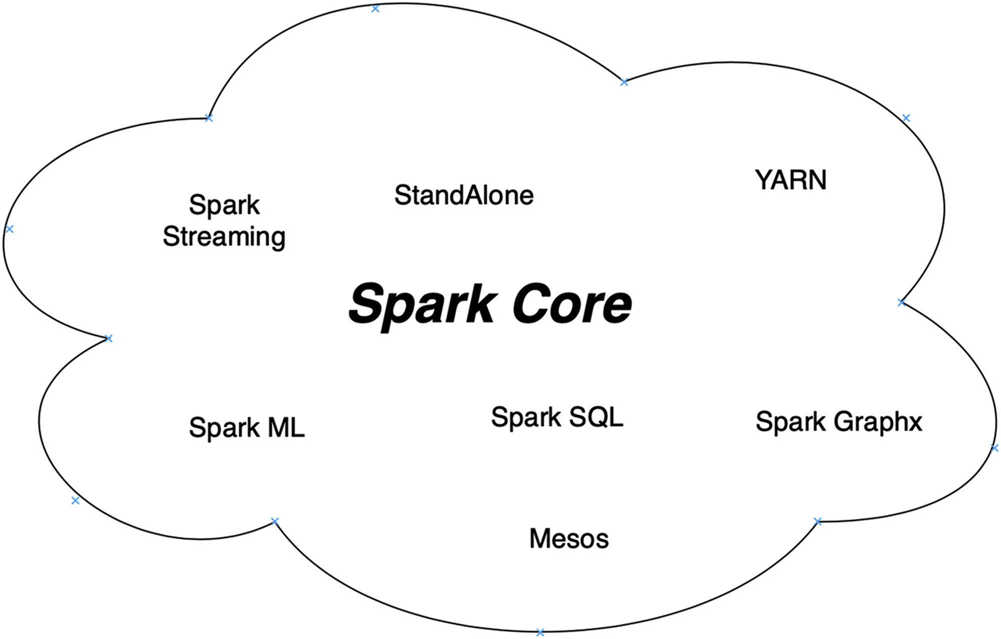
2.8.3. Apache Spark
This is a unified distributed computing engine for different platforms and workloads. Apache Spark can easily pair up with different platforms and process different data workloads using various paradigms, for example, Spark ML, Spark SQL, and Spark Graphx.
Apache Spark is very fast because of the in-memory data processing mechanism with suggestive application programming interfaces, which allow data handlers to accurately process machine learning or SQL workloads that need quick and interactive connection to the database.
Various other libraries are built on the core, which collectively allow loads for SQL, streaming, machine learning, and graph processing. For example, Spark ML has been devised for data scientists and its abstracted levels make data science very easy.
Spark provides machine learning, queries, real-time streaming, and graph processing. These tasks are quite difficult to perform without Apache Spark. We need to use various technologies for these different types of workloads, for example:
Apache Spark can do all of this, whereas multiple technologies are not always integrated. One more advantage of Apache Spark is that you can write client programs using various languages of your choice, i.e., Scala, Java, R, Python.
Apache Spark has some key advantages over the MapReduce paradigm:
Hadoop and Spark are prominent big data frameworks, but they are not used for the same purpose. Hadoop provides shared storage, MapReduce distributes computing frameworks, and Spark is a data processing framework that operates with distributed data storage given by other technologies.
It should be noted that Spark is quicker than the MapReduce Framework due to the data processing rate. Spark engages with datasets much more efficiently than MapReduce because the performance improvement of Apache Spark is efficient for off-heap-in-memory processing rather than solely relying on disk-based computations.
When your reporting requirements and data methods are not changing, then MapReduce's style of processing data may be sufficient, and it is definitely acceptable to use batch processing for your purposes. But if you would like to operate with data analytics on cascaded data or processing requirements for multistage processing logic, then you need to use Spark (Fig. 2.6).
2.8.3.1. Visualizations using tableau
When we perform distributed computing on big data, it is quite hard to comprehend the meaning of the datasets without tools like Tableau, which provides a graphic interface to the data in the dataset for better understanding and visualization of the data. There are other tools for the same purpose, such as Python's matplotlib, JavaScript, Cognos, KineticaDB, R+ Shiny, etc. Figs. 2.7 and 2.8 are screenshots of geospatial views of data using various tools for visualization.
2.9. Data warehouse versus data lake
Data structure:
Data lakes (Fig. 2.9) generally have unprocessed or raw data, while data warehouses store refined and processed data. Due to this, data lakes usually occupy more space than data warehouses (Fig. 2.10).
Moreover, data lakes are quite flexible, hence they can be analyzed swiftly and are ideal for machine learning.

Because of this, some risks also arise, one being the conversion of data lakes into data swamps without appropriate quality measures and data governance.
Purpose of data:
The use of various data chunks in data lakes is not static. Raw data combines with or forms a data lake just to have it handy or for some future purpose. This also means that a data lake has less filtration and less organization than a data warehouse. Data warehouses store processed and organized data, hence storage space is not wasted.

Users:
Raw, unstructured data cannot be easily understood by business professionals, but can be easily transformed, which is easily understood by anyone. Processed data is usually represented in charts, e.g., pie charts, etc., which can be easily understood.


Accessibility:
Accessibility refers to the database collectively. Data lakes do not have a definite pattern and hence are quite easy to control, use, and alter. Any modifications may be done easily and quickly because data lakes have fewer limitations.
Data warehouses are well ordered and hence are difficult to modify.
One major advantage is that the order and operation of data in a warehouse make the data itself very easy to decipher. It is very difficult and costly to manipulate data warehouses due to their limitations.
3. Introduction
3.1. What is data mining?
Databases today can be as large as several terabytes in size. In these vast clusters of data there remains concealed information, which can be of strategic importance. But how does one find a needle in these heaps of haystacks?
Data mining is a multidisciplinary field that responds to the task of analyzing large databases in research, commerce, and industry. The aim is to extract new knowledge from databases where complexity, dimensionality, or the sheer amount of data is so exorbitantly large for human analysis to be viable. It is not confined to the creation of models that can find particular trends in data either; it also deals with why those trends impact our business and how to exploit it. Data mining can be viewed as an interactive process that requires the computational efficiency of modern computer technology coupled with the background knowledge and intuition of application experts.
Now that we know what data mining is, the reader may still wonder what are the individual steps involved in this process.
The data mining process can be represented as a cyclic process that can be broadly divided into six stages as shown in Fig. 2.11.

This cycle is referred to as CRISP-DM (CRoss Industry Standard Process for Data Mining) [7].
The six stages of the CRISP-DM cycle are:
- 1. Business understanding: This stage deals with analysis of the task objectives and requirements from a commercial sense, and then this knowledge is used to create a data mining problem definition and a preliminary plan of action.
- 2. Data understanding: This stage begins with preliminary data gathering and proceeds with experimentation to become familiar with the data, to identify major problems with the data, to learn the first insights in the data, or to detect useful subsets that may help in forming useful hypotheses for the unknown data.
- 3. Data preparation: This stage involves all activities that lead to the transformation of the original raw data to obtain the final dataset.
- 4. Modeling: In this stage, various modeling methods are chosen and tested. But some methods like decision trees and neural networks have specific conditions concerning the form of the input data. Thus one may have to cycle back to the data preparation stage to obtain the required data in a suitable format.
- 5. Evaluation: Also called “validation,” this stage deals with testing model performance. After single or even multiple models have been constructed that perform satisfactorily based on the chosen loss functions, these models need to be tested to ensure that they maintain a satisfactory performance even against unseen data and that all crucial commercial concerns have been adequately resolved. The result is the selection of those model(s) that are able to give optimum results.
- 6. Deployment: Normally, this stage includes deploying a code equivalent of the selected model to estimate or classify the new data as it comes and to define the machinery that will use this new information in the solution for the initial business task.
The models used in data mining can be broadly divided into the following two categories: descriptive models and predictive models. Descriptive models are used to describe trends in existing data, and are usually used to generate meaningful subgroups such as demographic clusters, i.e., a model that can show regions where sales have been more frequent or of higher value. These types of models are based on unsupervised learning. Predictive models are often utilized to estimate particular values, based on patterns deduced from previously known data, i.e., supervised learning. For example, using a database containing records of previous sales, a model could be constructed that estimates an increase/decrease in sales of a particular group of products.
Now that we have understood what data mining is, let us have a look at what role machine learning plays in it.
3.2. Why use deep learning in data mining?
As you may have guessed after looking at the CRISP-DM cycle, machine learning has an important application in the modeling stage of the cycle. As previously stated, data mining usually deals with databases that are exorbitantly large for manual analysis. Hence, machine learning provides the set of tools required for an extensive analysis of such databases.
Even then, one may ask, why should one prefer deep learning algorithms over other machine learning algorithms for data mining? Let us take a look at the argument in favor of deep learning.
Traditional machine learning algorithms face what Richard Bellman had coined the “curse of dimensionality.” This states that with a linear increase in dimensionality of the data, the learning complexity grows exponentially, i.e., a small increase in dimensionality of data results in a large increase in learning complexity. Considering that real-world databases usually consist of high-dimensional data, the learning complexity is exceedingly large such that it is not practical to apply these algorithms directly to unprocessed data.
To combat this hurdle, feature extraction is often applied to the data. Feature extraction refers to a process used for dimensionality reduction in which the original set of raw data is reduced to a smaller, more compact subset that is easier to process, i.e., it refers to the methods that select and/or combine variables into features, thus reducing the total data that needs to be processed, while still accurately and completely describing the original dataset. But, since these are human-engineered processes, they can often be challenging and application dependent. Furthermore, if features extracted from the data are inaccurate or incomplete, the classification model is innately limited in its performance. Thus it becomes quite challenging to automate the process for application in data mining.
On the other hand, deep learning algorithms do not require explicit feature extraction on data before training. In fact, several deep learning algorithms, such as autoencoders, self-organizing maps (SOMs), and convolutional neural networks (CNNs), are implicitly able to select the key features to improve model performance. This makes them more suitable for use in data mining.
4. Applications of deep learning in data mining
4.1. Multimedia data mining
With the gaining popularity of the usage of multimedia data over the internet, multimedia mining has developed as an active region for research. Multimedia mining is a form of data mining wherein information is obtained from multimedia files such as still images, video, and audio to perform entity resolution, identify associations, execute similarity searches, and for classification-based tasks. It has applications in various fields, including record disambiguation, audio-visual speech recognition, facial recognition, and entity resolution. Deep learning has been essential in the progress of various subject areas, including natural language processing and visual data mining.
A task often faced in multimedia data mining is image captioning. Image caption generation is the process of generating a descriptive sentence for an image, a task that is undeniably mundane for us humans, but remains a problematic task for machines. The caption generation model deals with two major branches of machine learning. First, it must solve the computer vision problem of identifying the various objects present in the given image. Second, it also has to solve the natural language processing problem of expressing the relation between the visual components in natural language.
A novel approach for tackling this problem has been discussed in [8]. The model consists of a CNN network, which is responsible for encoding the visual embeddings present in the image, followed by two separate long short-term memory (LSTM) networks, which generate the sentence embeddings from the encodings given by the CNN. What makes this approach unique is the usage of bidirectional long short-term memory (Bi-LSTM) units for sentence generation.
Fig. 2.12 is a diagram showing the internal components of an LSTM cell. It constitutes the following components: a memory cell Ct, an input gate It, an output gate Ot, and a forget gate Ft. The input gate is responsible for deciding if the incoming signal will go through to a memory cell or if it will be blocked. The output gate is responsible for deciding if a new output is allowed or should be blocked. The forget gate is responsible for deciding whether to retain or forget the earlier state of the memory cell. Cell states are updated by feeding previous cell output to itself by recurrent connections in the two consecutive time steps.
On analyzing the model one may ask the following questions. First, why do we use recurrent neural networks (RNNs) instead of other mainstream methods for sentence generation? Second, what benefit does the use of Bi-LSTM provide for this application? Let us try to answer these questions.

Mainstream methods used to solve the task of image captioning mainly compromise either the usage of sentence templates, or treating it as a retrieval task by finding the best matching sentences present in the database and using them to create the new caption. The problem with these approaches is that they face a constant hurdle in the creation of original and/or variable length sentences. Thus they may not be suitable for use on data sufficiently different from the training data, limiting their application in real-world scenarios. On the other hand, even relatively shallow RNNs have shown considerable success in the creation of original and variable length sentences.
Let us now look at how Bi-LSTM networks are better than unidirectional LSTM networks. In unidirectional sentence generation, the common method of forecasting the subsequent word Wt with visual context V and prior textual context W1:t−1 is to choose the parameters such that the value of logP (Wt|V, W1:t−1) is maximized. While a unidirectional model is able to account for past context, it is still unable to retain the future context Wt+1:T, which should be considered for evaluation of the previous word Wt by maximizing the value of logP (Wt|V, Wt+1:T). The bidirectional model overcomes this shortcoming that plagues both unidirectional (backward and forward direction) models by exploiting the past and future dependencies to generate the new caption. Thus making them more suitable for tasks of language generation.
4.2. Aspect extraction
Aspect extraction can be defined as a subfield of sentiment analysis wherein the aim is identification of opinion targets in opinionated text. For example, where a company has a database of reviews given for its various products, aspect extraction would be used to identify all those reviews where a user either liked a product or disliked a product.
Before we look at the deep learning-based approach, let us look at why the existing mainstream methods for aspect extraction are not sufficient. These include:
Linear discriminant analysis: While this is ideal for datasets with high dimensionality, it is not optimal for text sentiment analysis because it treats each word as an independent entity, thus failing to extract coherent aspects from the given text.
Supervised techniques: Herein, the task is treated as a sequence labeling problem. While there exist several algorithms capable of achieving high accuracy for such problems, the fact that they heavily rely on quality data annotation to give good results makes them nonviable for real-life application in data mining.
Rule-based methods: These rely on extracting noun phrases and use of modifiers to deduce the aspects being referred to. But, a major issue with this approach is limited scalability, i.e., this approach is more suited to small datasets as compared to large datasets. Thus it is not suitable for data mining.
A suitable approach mentioned in [9] talks about using an autoencoder setup that reconstructs the input text. But the latent encoding thus generated would itself be able to represent the aspects mentioned in the text. This proposed model has been termed attention-based aspect extraction (Fig. 2.13). Let us have a closer look at the model.
An example of the attention-based aspect extraction structure [9] starts with mapping the words that usually co-occur within the same context. These words are assigned to nearby points in the embedding space. This process is known as neural word embedding. Then, the word embeddings present in a sentence are filtered by an attention-based mechanism and the filtered words are used to construct aspect embeddings. The training process for aspect embeddings is quite similar to that observed in autoencoders, i.e., dimension reduction is used to extract the common features in embedded sentences and recreate each sentence as a linear combination of the aspect embeddings. The attention-based mechanism deemphasizes words that did not belong to any aspect, thus the model is able to concentrate on aspect words.
The architecture of the model can be divided into the following components:
- • Input sentence representation: word embeddings.
- • Encoded sentence representation: attention-transformed embedding.

Figure 2.13 Attention-based aspect extraction [5].  (2.1)
(2.1)

4.3. Loss function
The dot product of any two different aspect embeddings should be zero.
4.4. Customer relationship management
Customer relationship management (CRM) can be described as the process of managing a company's interactions with its present and potential clients. It improves business relationships with customers, specifically focusing on ultimately driving sales growth and customer retention by applying data analysis to recorded data from previous interaction of the businesses with their clients. The aim of CRM is to integrate marketing, sales, and customer care service such that value is added to both the business and its clients.
For a company to grow and increase its revenue, it needs to compete for the more profitable customers. Businesses are using CRM to add value to their products and services, which will allow them to attract the more profitable customers. One vital subset of CRM is customer segmentation, which refers to the process of assigning customers into sets based on certain shared features or needs. Customer segmentation gives businesses the opportunity to better adapt their advertising attempts to different audience subsets. This can help boost both product development and communication. Customer segmentation allows businesses to:
- • Select the communication channels that are most suitable to reach their target audience.
- • Test different pricing decisions.
- • Create and broadcast targeted advertisements that can have maximum impact on specific sections of customers.
- • Identify areas of improvement for existing products and services.
- • Identify the more profitable groups of customers.
Clustering algorithms have been extensively used to tackle the task of customer segmentation. Meanwhile, visualization techniques have also become a vital tool for helping to understand and assess the clustering results. Visual clustering can be considered an amalgamation of these two processes. It consists of techniques that are simultaneously able not only to carry out the clustering tasks but also to create a visual representation that is able to summarize the clustering outcomes, therefore helping in the search for useful trends in the data.
But when we analyze the data available, we realize that it is usually heterogeneous, spatially associated, and multidimensional. Due to these properties, the basic assumptions of conventional machine learning algorithms become invalid, making them usually highly unsuitable for this category of data. Thus we use deep learning-based algorithms to overcome these hurdles.
One of these algorithms includes the SOMs, which allow the emergence of structure in data and support labeling, clustering, and visualization. As humans are typically not apt at visualizing or detecting patterns in data belonging to high-dimensional space, it is necessary to project this higher-dimensional data into a two-dimensional map such that the input records that are more similar to each other are located closer to each other. When this projection is represented in a form of a mesh of neurons it is called an SOM. This allows the clustering results to be presented in an easy-to-understand way and to interpret the format for the user.
There are two different usages of SOM. The first type refers to the traditional SOM, which was introduced by Kohonen [10] in 1982. In this category of SOMs, each cluster in the data is matched to a limited set of neurons. These are known as K-means SOMs.
The second form of SOMs, which were introduced by Ultsch [11] in 1999, uses the mapping space as an instrument to convert the high-dimensional data space into a two-dimensional vector space, thus enabling visualization. These SOMs contain a huge number of neurons, growing as big as thousands or tens of thousands of neurons. These SOMs are able to represent the intrinsic structural features present in the data space, i.e., they allow these features to emerge, and hence are referred to as emergent SOMs. The emergent SOM utilizes its map to visualize the spatial correlations present in the high-dimensional data space and the weight vectors of the neurons are used to represent a sampling point of the data.
Fig. 2.14 is a helpful visualization of the training process of an SOM.
The blue (dark grey in printed version) spot represents the training data's distribution, and the white grid-like structure represents the current map state, which contains the SOM nodes. Initially, the nodes are placed randomly in space. The distances of these nodes are calculated. The node that is nearest to the training datum (highlighted in yellow [light grey in printed version]) is chosen and shifted toward the training datum, as are its neighboring nodes on the map. But the displacement of these neighboring nodes is relatively smaller. This changes the shape of the map as the nodes on the map continue to be pulled toward the training datum. As the grid gradually changes, it is able to closely replicate the data distribution (right) after numerous iterations.

Functioning in an SOM can be divided into two parts:
The following formula is used to obtain the mappings:
where j, i ∈ I, i ∈ [1, M], and j ∈ [1, N] mi refers to the network's reference vectors, xj refers to the input data vectors, and mb refers to the best-matching unit.
The reference vectors are updated using the following formula:
 (2.7)
(2.7)where t represents the time coordinate with discrete intervals and hib(j) is a reducing function of time and neighborhood radius.
Each unique unit formed in an SOM can be viewed as an individual cluster. When visualizing, it is preferable to have a large number of neurons as it leads to increased projection granularity (i.e., detail). But, increasing the number of neurons incessantly can lead to the processing of the SOM resembling the process of data compression into a characteristic set of units rather than standard cluster analysis, thus hindering the interpretability of the data presented by the clusters. Thus these SOM units are collected into clusters by applying a second-level clustering. In a two-level SOM, the SOM is used to project the initial dataset onto a two-dimensional display. This is followed by clustering the SOM units.
Previous research has proved the effectivity of the two-level SOM technique; among these, Li H [13] has shown the higher effectiveness of the combined approach of both the SOM and Ward's hierarchical clustering, compared to several conventional clustering algorithms.
We can describe Ward's clustering [14] in the following manner. It starts by treating each unit as a separate cluster on its own. Then, we proceed by selecting the two clusters that have the minimum distance and merging them. This step is repeated until there is a single cluster left. Ward's clustering can be restricted such that only the neighboring units are merged to conserve the spatial ordering of SOM. The Ward distance can be modified in the following manner to reflect the new clustering scheme [14]:
where l and k represent clusters, Dkl represents modified Ward distance between the two clusters,  represents the squared Euclidean distance between the cluster centers of clusters l and k, and nl and nk represent the cardinality of clusters l and k, respectively. Also, we consider the distance between two nonadjacent clusters to be infinity. Thus when clusters l and k are merged to form a new cluster z, the cardinality of z can be defined as the sum of the cardinalities of l and k and the centroid of z is the mean of cl and ck weighted by their cardinalities.
5. Conclusion
In this chapter, we focused on two major topics: big data and data mining. We learnt about the two fundamentals of data analytics, i.e., EDA and CDA. Then, we focused on the seven Vs of big data, which are equivalent to the basic definition of big data. Then, we took a deep dive into distributed computing and why it is important for big data analytics and various frameworks for big data analytics such as MapReduce Framework and Hive. Then, we studied Apache Spark and why is it better to analyze data using it. After this we covered visualizations of the processed data and why it is important, and various technologies used for data visualizations. Then, we learnt about the difference between data lake and data warehouse and which is better for a particular group of people. We talked about some of the limitations of both data lakes and data warehouses. We also tried to answer questions like “What is data mining? Why is deep learning used in data mining? What are some real-world applications of deep learning in data mining?” We now understand why deep learning algorithms are more suitable than other mainstream machine learning algorithms for application in data mining and to that effect we studied their application in real-world problems in the form of Bi-LSTM for multimedia data mining, ABAE for aspect extraction, and SOM for CRM.
We have tried to give a brief introduction to the various applications and the mathematics involved in them; however, this is by no means a complete guide. The author would recommend the reader to see the references for sources to enable further in-depth study of the techniques discussed in this chapter.
..................Content has been hidden....................
You can't read the all page of ebook, please click here login for view all page.