
Chapter 11: Deep learning-based detection and classification of adenocarcinoma cell nuclei
G. Kalyani1, and B. Janakiramaiah2 1Department of Information Technology, Velagapudi Ramakrishna Siddhartha Engineering College, Vijayawada, Andhra Pradesh, India 2Department of Computer Science and Engineering, Prasad V. Potluri Siddhartha Institute of Technology, Vijayawada, Andhra Pradesh, India
Abstract
Nowadays, clinical practice uses digital pathology for examining digitized microscopic images to identify diseases like cancers. The main challenge in examining microscopic pictures is the need to dissect every single individual cell for precise analysis because identification of cancerous diseases depends emphatically on cell-level data. Due to this reason, the detection of cells is a significant point in medical image examination, and it is regularly the essential prerequisite for disease classification techniques. Cell detection and then classification is a problematic issue because of diverse heterogeneity in the characteristics of the cells. Deep learning methodologies have appeared to deliver empowering results on analyzing digital pathology pictures. This chapter introduces an approach by using region-based convolution neural networks for locating the cell nuclei. The region-based convolution neural network estimates the probability of a pixel belonging to the core of the cell nuclei. Pixels with maximum probability indicate the location of the core of the cell nucleus. After finding the cells, they are classified as healthy or malicious cells by training a deep convolution neural network. The proposed approach for cell detection and classification is tested with the adenocarcinoma dataset. Cell image analysis based on deep learning techniques shows good results in both the identification and classification of the cell nucleus.
Keywords
Cell classification; Cell detection; Convolution neural network; Deep learning; Medical image analysis
1. Introduction
An aggregate term for uncontrolled threatening tumor development occurring in any tissue of the body is cancer. More than 100 kinds of tumors have been recognized to date. Some of them are explicitly based on gender, and others are not. Different types of malignant growth in the lungs, colon, and blood are commonly found in humans. Medical procedures like radiotherapy, chemotherapy, and surgery are the built-up procedures for treating cancer disease, but may also have critical symptoms as side effects. In any case, 100% healthy outcomes due to heterogeneity and immunity of tumor cells to available treatments of cancer disease have yet to be established. At the same time, tumors are known for their complex varieties that makes it hard for doctors to identify the strategy for treatment. Hence, it is progressively becoming an essential task to identify a given tumor and prove the location of the cancer and the phase it is at to continue “customized” treatment.
A carcinoid tumor is a well-separated neuroendocrine tumor that 55% of the time regularly starts in the gastrointestinal tract, or in different areas, for example, the lungs, kidneys, or ovaries. Tumors include a very high level of cell heterogeneity because of their capacity to inspire shifting degrees of fiery host reaction, angiogenesis, and tumor rot among different variables associated with tumor advancement [1]. The location of these various cell types has additionally been demonstrated to identify the malignant growth grades [2]. Subsequently, the subjective and quantitative examination of various kinds of tumors at a cell level not only helps to better comprehend a cancer but also to investigate different choices for the treatment of the disease. One approach to studying cell types is by utilizing various protein markers that identify multiple cells in malignant tissues.
Manual examination of microscopy pictures analysis by the manual process isn’t just tricky and also costly but on the other hand, is biased with the inconsistencies based on the person who is examining the picture. Gurcan et al. [3] demonstrated that digitized example investigation could substantially make the objectivity and reproducibility of computer-assisted diagnosis better. In that type of case, programmed and robust cell identification are profoundly appealing and become essential for a wide assortment of ensuing tasks, for example, cell division and morphological estimations [4]. Also, the blend of cell recognition and a consecutive phase of classifying cells can give clinically relevant data about objects of intrigue, for example, the existence (or amount) of malignant growth in cells in a microscopy picture.
Cell detection is the process of discovering the presence of a particular sort of cell in a microscopy picture. Detecting cells is a noteworthy objective in a broad scope of applications with clinical images. Tumor development speed is a significant biomarker indication for detecting cancers. In most situations the most extensively accepted technique commonly applied by pathologists is observing tissue slides using a microscope and considering their observational evaluations. Observations by pathologists are precise in a few cases, yet for the most part they are less so and can lead to misinterpretation. Cell recognition and localization establish a few difficulties that require consideration. The initial challenge is that target cells are not simple structures but comprise complex structures such as vessels, collagen, and so on. The volume of the intended cell is tiny, and thus it tends to be difficult to identify cells from the previously complex structures. The other challenge is that objective cells can show up sparsely (in tens), modestly thickly (in several hundreds), or exceptionally thickly (in thousands) in a microscopy picture, as shown in Fig. 11.1 [5]. Furthermore, noteworthy varieties in the appearance of target cells can likewise be possible. These difficulties make cell identification/confinement/checking issues difficult to perform, regardless of notable advances in the research of computer vision.
After the success of deep learning, research has been conducted to detect objects in a picture. Nevertheless, the task of cell identification is not the same as general objects detection in a picture such as detecting persons and vehicles, which occupies a considerable space in the given image. Region-based convolution neural networks (CNNs) [7] and their variations [6] and fully convolution networks with optimization [8] have become the best-in-class algorithms for the issue of object detection. However, these techniques are not meant for cell identification because of doubts and difficulties. For instance, for general objects, localization is viewed as fruitful if a recognition location box is half covered by the exact location region. For cell identification, tolerance is commonly required in a much tighter bound to make identification meaningful.

2. Basics of a convolution neural network
A CNN or ConvNet is an exceptional sort of multilayer neural network. CNNs mostly take images as input, which permits the user to encode a few properties of the network, thus dropping the number of parameters. Generally, there are three main layers in a simple ConvNet: convolution layer, pooling layer, and fully connected layer. The input layer holds the image data. Fig. 11.2 demonstrates the general structural design of a CNN with various layers.
2.1. Convolution layer
The principal layer in a CNN is the convolution layer, in which every neuron is associated with a specific region of the area related to the input called the receptive field. The main objective of convolution concerning ConvNet is to take out the features from the given image. This layer does most of the computation in a ConvNet. The result of every convolution layer is a set of feature maps, created by a solitary kernel filter of the convolution layer. These maps can be characterized as input to the following layer.

A convolution is an algebraic operation that slides a function over other space and measures the essentials of their location-based multiplication of a value-wise product. It has profound associations with Fourier and Laplace transforms and is intensely utilized in processing the signals. Convolution layers utilize cross-relationships, which are fundamentally the same as convolutions. In terms of mathematics, convolution is an operation with two functions that deliver another function—that is, the convoluted form of one of the input functions. The generated function gives an integral of the value-wise product of the two given functions as an element of the sum that one of the given input functions deciphered.
The architectural design of ConvNet enables the system to focus on low-level highlights first, and afterward collect them into more significant-level highlights in the following hidden layers. This type of various-leveled structure is regular in natural pictures, which is the reason for the functioning of CNNs for recognizing the images. A convolution layer in Keras has the following syntax:
Conv2D(filters, kernel_size, strides, padding, activation = “relu,” input_shape)
Arguments in the foregoing syntax have the following implications:
- • Filters: The number of filters.
- • Kernel_size: A number specifying both the height and width of the (square) convolution window. Some additional optional arguments might be tuned.
- • Strides: The stride of the convolution. If the user does not specify anything, it is set to 1.
- • Padding: This is either valid or the same. If the user does not specify anything, the padding is set to valid.
- • Activation: This is typically ReLu. If the user does not specify anything, no activation is applied. It is strongly advised to add a ReLU activation function to every convolution layer in the networks.
It is possible to represent both kernel_size and strides as either a number or a tuple. When using the convolution layer as a first layer (appearing after the input layer) in a model, you must provide an additional input_shape argument—input_shape. It is a tuple specifying the height, width, and depth (in that order) of the input. Make sure that the input_shape argument is not included if the convolution layer is not the first layer in the network. Fig. 11.3 illustrates an example of convolution with filter size 2 × 2 with a stride of 2.

In CNN, the behavior of the convolution layer is controlled by specifying the number of filters and dimensions of each filter. The number of nodes in a convolution layer is increased by enhancing the quantity of filters. Dimensions of the filters are to be enhanced to enlarge the size of the pattern. There are also a few other hyperparameters that can be tuned. One of them is the stride of the convolution. Stride is the amount by which the filter slides over the image. The stride of 1 moves the filter by 1 pixel horizontally and vertically. Here, the size of the convolution becomes the same as the width and depth of the given input image. The stride of 2 makes a convolution layer half the given input dimension. If the kernel filter moves outside the image, then we can either ignore these unknown values or replace them with zeros.
2.2. Pooling layer
As we have seen, a convolution layer retrieves the feature maps, with one feature map for each filter. More filters increase the dimensionality of convolution. Higher dimensionality indicates more parameters. So, the pooling layer controls overfitting by progressively minimizing the spatial size of the feature map to reduce the quantity of parameters and calculations. The pooling layer often takes the convolution layer as input. Every neuron of the pooling layer is linked to a few neurons of the preceding layer, which is positioned in a receptive field, i.e., specified as a rectangular region. However, size, stride, and type of padding are specified for that region. In other words, the aim of using pooling is to reduce a load of computation, usage of memory, and the number of parameters by subsampling the input image. It helps the model from overfitting in the phase of training. Lessening the image size of the input additionally causes the neural system to endure a slight picture shift. The spatial semantics of the convolution operations rely upon the scheme of padding picked.
The operation of padding is to expand the size of the information. On account of 1D information, a constant is added to the array; in 2D information, the constants are used surrounding the input matrix. In n-dimensional data, the n-dimensional hypercube is surrounded by a constant. To a maximum extent, the constant used in the padding is “0.” Hence, it is called zero padding. There exist other types of padding techniques like “VALID” padding and “SAME” padding. “VALID” padding drops the rightmost columns or bottom-most rows. In the case of “SAME” padding, data is padded evenly on the right and left. If the padded columns are odd, then an additional column is appended to the right.
Selecting the operation for pooling plays a significant role in the pooling layer. The pooling operation is like the filter applied to the feature map. Hence, the filter size should be less than the feature map size. Explicitly, it is quite often 2 × 2 size, with stride 2. This implies that the pooling layer will consistently diminish the size of every feature map to half of its original size. The most generally utilized pooling approach is max pooling. Along with max pooling, pooling layers can also implement other pooling operations like mean pooling and min pooling.
The most extreme pooling, i.e., max pooling, considers the most significant pixel value in each filter patch of the feature map. The outcomes are downtested or pooled maps that feature the brightest element in the filter patch. Max pooling selects the bright features in the given image. For the task of classifying the images in the domain of computer vision, max pooling presents the enhanced results when contrasted with the other pooling operations. Max pooling provides improved results if the image is white on a black background. Fig. 11.4 illustrates the operation of max pooling.
Average or mean pooling performs the calculation of the mean of all the values in a filter patch, which are applied to the feature map. This implies that each 2 × 2 square of the filter is examined to the usual incentive in the square. The mean pooling technique smooths out the picture, and thus the sharp highlights may not be recognized. Fig. 11.5 illustrates the operation of mean pooling.
The minimum pooling or min pooling operation considers the minimum or smallest value in every patch of the feature map. Min pooling presents enhanced results in the case of images on a white background. Fig. 11.6 illustrates the operation of min pooling.


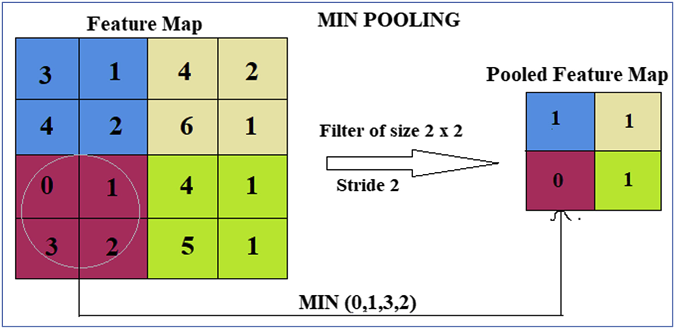
Fig. 11.7 shows the difference between these three pooling methods with an example picture resulting in max pooling, average pooling, and min pooling for a given original picture.
2.3. Fully connected layer
The set of convolution and pooling layers acts as the feature extraction part in the CNN. The retrieved features are processed to classify or detect the objects in the image. The final few layers of the ConvNet are fully connected layers for detection purposes. Fig. 11.8 illustrates the fully connected layers.


Fully connected layers simply work as a feed-forward network. The result of the last pooling is in the form of a matrix. It is converted into a vector with a technique called “flattened” and is considered as input to these layers. The process of flattened is shown in Fig. 11.9.
Fully connected layers compute the mathematical operations as follows:
where:
A stands for activation function
W indicates weight matrix of dimension M × N
M indicates neurons of the preceding layer
N stands for neurons of the succeeding layer
X represents the input vector obtained from the flattened process of size N × 1
b denotes the vector of bias.
The computation is carried out in every layer. All the fully connected layers make use of ReLu as the activation function. After processing through fully connected layers, in the final layer instead of ReLu a function called softmax function is implemented. This function gives probabilities of the input related to every label. The utmost probability node indicates the label of the considered input.
3. Literature review
Identifying objects in a familiar scene generally yields a set of rectangular boxes to specify the position and volume of recognized substances. R-CNN [9] and YOLO [10], along with their variations, use the aforementioned rectangular box indication. Some of the broadly utilized methods for object detection utilize marking in boxes, such as OTB [11] and COCO [12]. Indicating an entity with a carton of four boundaries, the quantity of yield hubs in entity identification has decreased. For marking the cells, the spots at the center of the cell and the curved outline shape of cells are generally used. The curved outline shape incurs additional time when compared to center dot labeling; the latter is the widely used marking strategy for detecting cells. In cell identification strategies that rely on learning, initial labels are preprocessed and then only used as data to train the model. Dividing the entire image into little fixes [13] and changing the dots into a density indication [14] are two standard methodologies.
Over the last couple of decades, various methods for cell detection have been proposed [15]. Cell detection methods based on computer vision use basic techniques for processing images, such as thresholding on intensity, identification of features, morphological separating, accumulating the regions, and model fitting. In these cases, conventional approaches for cell detection based on architecture comprise significant feature determination followed by a classifier. In the first phase, the system disengages one or more highlighted features as the picture representation. Conventional methods for processing the images offer scope for the selection of highlighted feature extraction techniques. Later on, machine learning was developed, which works as a classifier, feature selector, and identifies the regions that contain identified cells. However, the aforementioned conventional approaches have limitations. The first one is that manually selecting the essential features is a difficult task. Much of the time this requires critical information about the targeted cells in advance. The second is that features may contain numerous parameters that have a significant role in the performance of a task. Hence, users have to spend more time with trial and error methods to tune those parameters. The third one is that all the features will not play the same role on the targeted cells, i.e., the essential features may change from one target cell to another. The most important limitation is that the accuracy of the classifier selected with the manually selected features may not always be better when compared to accuracy with all the input features.
To overcome these limitations, cell detection based on deep learning has been proposed. In the computer vision domain, the best-in-class strategies in cell identification depend on deep neural systems. The primary thought behind these techniques is that models are prepared as a classifier in picture space as a pixel-naming [16] or as a region [17] network. Therefore the strategies anticipate the horizontal and vertical directions of cells legitimately on a 2D picture. Nowadays, deep neural systems are used for an extensive range of problems in computer vision and have accomplished better accuracy on benchmark datasets in the corresponding domain [18]. The most convincing benefit with deep learning is the usage of an advanced form of fixed component plan methodologies toward automatic learning of issue-explicit highlights simply from training information [19]. By providing vast amounts of images and related labels as the training data, clients do not need to pay much attention to the detailed strategy for the retrieval of highlights. As an alternative, the deep neural system is developed by applying the gradient descent technique on the training data, so the deep neural systems facilitate the autonomic learning of associations in the information. For instance, upper layers of deep neural systems concentrate on adapting low-level highlights, while deep layers of deep neural systems concentrate on progressively dynamic elevated-level semantic portrayals.
Cires et al. [20] introduced a methodology based on CNN for detecting cells. The anticipated network consisted of a 12- and 10-layer network, and in detection attained a computation speed of 0.01 and 0.03 megapixels per second. Another way of classification with CNN consists of 8 layers. AlexNet [21] was utilized by Janowczyk et al. [22] to identify lymphocytes in the images related to breast cancer. Khoshdeli et al. [23] utilized a five-layer deep network for identifying the nuclei in hematoxylin and eosin (H&E)-marked metaphors of a variety of tissue types. They filtered the given images by extorting the hematoxylin based on a Laplacian or Gaussian filter, and the outcome was subsequently given to the network.
Cell checking and recognition are executed by a CNN pursued by a compressive detecting module [24]. An image of size 200 × 200 pixels containing dissimilar cells was given as input to the CNN. The outcome was a vector “z” that included compacted focus area data. The compressed area data was estimated by framing a matrix “S” with “z = S ∗ x,” in which “x” is an input vector. The size of “z” should not be more than the size of the “x”. Previously, compressed sensing based output encoding was used along with the predictors of linear and non linear type. The idea of coding the basic cell locations was addressed in [24], by using compressed sensing which is not exactly the same as spatial channel coding. To begin with, the detecting framework S was an additional mapping connection by the neural system. Due to the size of S, much preparing of information was required to avoid overfitting and maintain exactness. Second, recouping the area data from the compacted vector can be tedious.
Henning Höfener et al. [25] trained CNN to create a PMap, which was considered as either a classification or a regression task. Taking into consideration the classification task, two classes existed, i.e., nucleus center and background. In the training phase, the classes were considered as discrete values 1 and 0. The probabilities corresponding to the class nuclei center were considered as values of the PMap. Later, location of the nuclei centers was identified by calculating the local maxima of PMap that go beyond a certain threshold. An area of identical values in which the entire adjacent pixels contain reduced values compared to other areas was considered as local maxima. The local maxima may be as small as a single point. The fundamental PMap approach was managed with the number of parameters. The authors concentrated on efficient listing, estimation, and comparison of those parameters. The effect of individual parameters concerning accuracy of detection, efficiency, and effort required for training was assessed. Finally, the authors merged individual parameter settings, which achieved ideal results in the experimentation for final evaluation.
Chowdhurya et al. [26] used a pretrained AlexNet network, trained on the ImageNet dataset, for retrieving the features based on which colon cancer can be detected. The extracted features were united with the manually selected features by particular persons who were the feature extractors. They used a support vector machine for the detection of colon cancer. Kashif et al. designed a model with CNN based on spatial constraints for the identification of tumor cells in histology images [27]. By applying the spatial constraints, two layers were included in the general CNN architecture, which were designed for extracting color characteristics and texture information. The automatic extraction of features with deep learning was proposed by Xu et al. [28]. Two frameworks based on CNN were introduced for learning the features, which were fully supervised and unsupervised, respectively. Haj-Hassan et al. [29] projected a method by training a CNN using segmentation results. The trained CNN was used to classify the colorectal cancer tissues from multispectral images [29]. Table 11.1 summarizes the work reviewed in this section for adenocarcinoma detection.
4. Proposed system architecture and methodology
The outline structural design of the methodology is illustrated in Fig. 11.10. The proposed architecture comprises mainly two phases: (1) cell detection with Faster R-CNN and (2) cell classification with ResNet101. H&E-stained images are taken as input images. The output is whether the image contains cancerous cells or not. Hence, the final task is a binary classification task of having cancer cells or not having cancer cells.
Table 11.1
| References | Application | Architecture used | Learning type |
|---|---|---|---|
| Hao Chen [17] | Cell detection | Deep neural network | Design and training |
| Cires et al. [20] | Cell detection | CNN | Design and training |
| Janowczyk and Madabhushi [22] | Identifying lymphocytes in breast cancer images | CNN | Transfer learning |
| Khoshdeli et al. [23] | Checking nuclei in hematoxylin and eosin marked metaphors | Deep neural network | Design and training |
| Y. Xue [24] | Cell checking and recognition | CNN | Design and training |
| Henning Höfener et al. [25] | Identification and classification of nuclei | CNN | Design and training |
| Chowdhurya et al. [26] | Grade classification in colon cancer | CNN | Transfer learning |
| Kashif et al. [27] | Detection of tumor cells | CNN | Design and training |
| Xu et al. [28] | Feature learning with minimum manual annotation | CNN | Design and training |
| Haj-Hassan et al. [29] | Classification of cells corresponding to colorectal cancer | CNN | Design and training |


The algorithm of the proposed methodology consists of the following steps:
- Step 1: Load the image dataset
- Step 2: Adjust the training and test sets
- Step 3: Detect the cells with Faster R-CNN
- Step 4: Prepare training images and test image sets
- Step 5: Load the pretrained ResNet-101 model
- Step 6: Train the ResNet-101 with the training data
- Step 7: Evaluate the classifier
- Step 8: Apply the trained classifier to test images
- Step 9: Evaluate the accuracy
4.1. Cell detection using faster R-CNN
The Faster R-CNN algorithm efficiently detects the cells in an image. The architecture of Faster R-CNN is shown in Fig. 11.11. The outline of Faster R-CNN is explained in the following steps:

- Step 1: Pass an input image to the convolution net of Faster R-CNN, which retrieves the feature map in the given input.
- Step 2: The identified feature map is the given to the region proposal network (RPN) of Faster R-CNN. The RPN receives the object proposals.
- Step 3: The identified object proposals are given to the region of interest (RoI) pooling layer to convert the object proposals of varying sizes into a uniform size.
- Step 4: The uniformly converted object proposals are passed onto the fully connected layers of Faster R-CNN. The fully connected layers place bounding boxes if the object proposal contains a cell that is different from the background.
The input for Faster R-CNN is an image and it is processed with four modules. It consists of a feature extraction network, RPN, RoI pooling layer, and R-CNN. RPN aims to adjust anchor boxes with the original bounding boxes. The R-CNN for calculating the bounding box regression values and classifying the bounding box as the box that contains cells or the box does not contain the cells. RPN and R-CNN share convolution layers to save time.
For extracting the original features in the given input image, we used a VGG16 network to attain better feature extraction performance. VGG16 is a CNN model presented by the University of Oxford [30]. VGG16 is a convolution layered model to extract the sophisticated features even though the training dataset consists of smaller instances. The outline architecture of VGG16 is shown in Fig. 11.12. VGG16 is used because the network will use fewer hyperparameters. The convolution layers are based on filters of size 3 × 3 with a stride of 1. The pooling layers are implemented with the SAME padding and filters of size 2 × 2 with a stride of 2.

The features extracted by the VGG16 are used in RPN to produce the object proposals. The idea for obtaining the region proposals of the objects is the concept of anchor boxes. Anchor boxes are the bounding box assigned for every pixel in the feature map, and the network will try to search for the best counterbalance from the coordinates of the anchor box to fit the nearest enclosing object directed by a loss function. The output of RPN is a set of boxes that are checked by a classifier to confirm the incidence of objects, i.e., cells eventually. To be exact, RPN forecasts the likelihood of an anchor box as a background or foreground, and refines the anchor.
After RPN, the marked regions are available with varying sizes. The regions of varying sizes imply CNN feature maps with varying sizes. It is difficult to make a productive structure with feature maps of various sizes. RoI pooling solves the issue by converting all the feature maps into a similar size. RoI pooling divided the highlighted feature map as a predetermined number (supposedly k) of regions with equal size and afterward used max pooling for each part separately. Hence, the result of RoI pooling does not depend on the input feature map size.
After RoI pooling, the similarly sized regions are given to the R-CNN classifier to categorize them as either the foreground, i.e., containing cells, or the background of the image. In the medical images, the foreground means the presence of cells in that part of the medical image.
4.2. Cell classification with ResNet-101
The detected cells are classified by using a deep network, which is meant for classification. Here, we use the ResNet-101 network for classification [31]. The pretrained net is adjusted with our training data. ResNet-101 is a residual network that solves the problem of vanishing gradient, which arises in deeper networks. With ResNets, the gradients can flow directly through the skip connections. The architecture of ResNet-101 is shown in Fig. 11.13. ResNet-101 consists of mainly five types of convolution blocks called conv-1, conv-2, conv-3, conv-4, and conv-5. Conv-5 is succeeded by a fully connected layer and softmax layer for output classification. Each convolution block makes use of three convolution layers of size 1 × 1, 3 × 3, and 1 × 1. ResNet-101 was able to classify images into 1000 categories, but we fine-tuned the model to classify the images into four categories.
5. Experimentation
This section elaborates on the dataset used for experimentation of the proposed algorithm and the results with the experimentation completed.

5.1. Dataset
Experimentation of the proposed methodology was done by considering an adenocarcinoma dataset, which is openly accessible by the Tissue Image Analytics Lab at Warwick, UK [32]. The dataset comprises 100 H&E images of adenocarcinoma tissues. The given input pictures have a resolution of 500 × 500, which corresponds to 20× visual magnification. Center marker indications exist for every nuclei in all the images. A skilled pathologist authenticates the marked observations of the images. A total of 29,756 nuclei is indicated for detection purposes. Among 29,756 nuclei, 22,444 nuclei have a related class label. The leftover 7312 nuclei are not labeled. The marked nuclei are classified into four classes. Fig. 11.14 shows samples of nuclei from the dataset related to four class labels [32].

5.2. Discussion on results
For robustly validating the proposed algorithm, the experimentation was carried out with the cross-validation technique. The dataset was partitioned as five disjoint folds. All the folds were of the same size. In every experimentation, the network was trained with four folds and validated with the remaining one fold. Hence, 80 images were considered for training the network, and 20 images were used for testing in every run of the experimentation. After testing, the values related to TP, FP, TN, and FN were added with respect to the complete test data in all the experiments, and the measure F1-score was evaluated:
where TP is the number of properly classified nuclei, TN indicates the correctly identified normal nuclei, FP is the number of infected nuclei recognized as normal nuclei, and FN is the number of normal nuclei recognized as infected nuclei.

In the proposed algorithm, the first part of Faster R-CNN first marks the nuclei in the given test image. Fig. 11.15 illustrates the result of the cell detection part of the projected methodology using Faster R-CNN. The left part of the figure, i.e., (A), demonstrates the original image given as an input, and the right side (B) is the image marked with the cells detected.
Later, the second phase of the proposed algorithm, the identified nuclei in the first step with Faster R-CNN, was given as input to the network, i.e., ResNet-101 network, to classify the patches and have the cells marked at the center as four classes: epithelial, inflammatory, fibroblast, and miscellaneous. To evaluate the efficiency of the classification phase, we calculated the F1-score measured by using the measures precision and recall. The outcomes of the proposed algorithm were evaluated with two of the existing methods called spatial constrained convolution neural network (SC-CNN) and stacked sparse autoencoder (SSAE) [32].
Comparison of the precision parameter is shown in Fig. 11.16. Fig. 11.16 demonstrates clearly that the precision has the values 0.617, 0.758, and 0.762 for SSAE, SC-CNN, and the proposed method, respectively. Comparison of the recall parameter is shown in Fig. 11.17. Fig. 11.17 demonstrates clearly that the recall has the values 0.644, 0.827, and 0.855 for SSAE, SC-CNN, and the proposed method, respectively. Comparison of the F1-score parameter is shown in Fig. 11.18. Fig. 11.18 demonstrates clearly that the F1-score has the values 0.63, 0.791, and 0.805 for SSAE, SC-CNN, and the proposed method, respectively. Table 11.2 shows the outcomes of the precision, recall, and F1-score for the existing SC-CNN, SSAE, and the proposed algorithm, respectively.


6. Conclusion
We demonstrated an automatic cell identification and classification framework using deep learning for processing medical images. The framework was mainly intended to resolve complex imaging scenarios concerning classification problems with multiple class labels, in which the cells in the input image can overlap with each other. For detecting the cell, we used the Faster R-CNN architecture, which involved feature extraction, region marking, and a classifier to classify that either the marked regions had cells or they were associated with the background of the picture. The second phase of the proposed framework was cell classification. We used the ResNet-101 framework by fine-tuning with our training data. The experimental results proved that Faster R-CNN with VGG16 efficiently detected the cells in the medical images. ResNet-101 classified the cell patches identified by Faster R-CNN efficiently.
..................Content has been hidden....................
You can't read the all page of ebook, please click here login for view all page.