
6
Resiliency on Temporal Scale
Minimal interruption of infrastructure service ensures the continuity of economic prosperity.
6.1 Principle 3
Resiliency is the ability of EEIS to cope, recover, or adapt to chronic or acute stressors due to system properties such as robustness, adaptive capacity/redundancy, rapidity, and resourcefulness. In a simple term, resiliency refers to the ability to absorb shock such as temperature, flooding, or droughts. A simple quantification of resiliency is the time that an EEIS recovers from a stressor event and loss of function. On temporal scale, EEIS should be resilient over 20, 50, and 100 years with quantified uncertainty and the sensitivity of the EEIS should be quantified on different temporal scales.
There are two types of stressors: chronic stressors include temperature increases and sea level rise, while acute stressors include extreme hurricane, earthquake, storm, tornados, cold weather, power outage, and wildfire. Resiliency was applied to ecology and engineering by Holling (1973, 1996); to socioecological systems by Walker et al. (2004); to WRRFs by Currie et al. (2014), Schoen et al. (2015), and Xue et al. (2015); to water supply system by Hwang et al. (2014); and to drainage systems by Mugume et al. (2014) and Goldbloom‐Helzner et al. (2015). Performance of EEIS includes effluent quality, level of service, unit energy consumption, waste production, and monetary loss. To quantitatively link the properties of EEIS to its performance, Cuppens et al. (2012) quantified resiliency as follows:

where
- tn is the total duration of the perturbation until recovery
- t0 is the initial time when the perturbation occurs
- M0 is the initial state of the chosen metric (a state variable representative of the state of the system)
- Mt is the value of the chosen metric at a measured time t
Francis and Bekera (2014) quantified resiliency in terms of function recovery of performance level using an equation that reflects three properties: absorptive (robustness), adaptive, and restorative (rapidity) as follows:
where
- Sp is the speed recovery factor
- Fo is the original stable system performance level
- Fd is the performance level immediately post‐disruption
- Fr is the performance at a new stable level after recovery efforts have been exhausted
Regardless of how to quantify the resiliency, it is critical to consider increase in resiliency as an opportunity and not an extra cost or effort. Indeed, Sweetapple et al. (2016) assessed the trade‐off between resilience and reliability. Resiliency is maximum failure time under different levels of stressors for WRRFs. Multiobjective optimization could be used to evaluate the cost function of an intervention to build resiliency. Optimal conditions could then be determined by balancing cost/benefit between resiliency implementation and reliability. For Miami‐Dade Water and Sewer Department (WASD), deep well injection does not increase resiliency of the system because it dispose 200 MGD treated wastewater effluent as deep as 10 000 ft. As a result, a reliable water resource from the reclaimed water would not be utilized. To decrease time to recover after major stress, Miami-Dade WASD will spend 13.6 billions to increase resiliency of it EEISs in next decade.
One of the most effective ways to quantify resiliency is to formulate different stressor scenarios and calculate the corresponding performance under different stressor scenarios. For example, Mabrouk et al. (2010) used mass balance of reactors and quantified the effect of influent variability on optimal design parameters of the reactors. Lempert et al. (2015) built a model of a system, developed sets of scenarios using Monte Carlo (MC) techniques, and assessed resiliency of the system in terms of specific performance metrics. To quantify the resiliency of WRRFs, Schoen et al. (2015) formulated failure profile for robustness, redundancy and recovery profile for resourcefulness, rapidity with consideration of lifespan of WRRFs. Weirich et al. (2015) applied a statistical method to avoid mathematical model of the system’s components. The WRRF performance was predicted using effluent concentration in generalized linear models (GLMs). Hwang et al. (2014) assessed the resiliency of water supply system under different scenarios such as centralized versus decentralized plants using linear programming (LP). However, quantitative benchmarks of metrics are needed to increase the resiliency of EEIS (Juan‐García et al., 2017). The metrics should include robustness, adaptive capacity/redundancy, rapidity, and resourcefulness of EEIS. Nevertheless, these methods provide quantitative way to assess resiliency of EEIS to future climate change and its resultant severe droughts and flooding on temporal scales.
Temporal scales have to be considered to reflect the economic development stage for current and projected time frame. For example, the recycling rate of solid waste is directly proportional to the GDP of a country. The higher the GDP, the higher the degree of separation and recycling. To increase the resiliency of stormwater management, green infrastructure should be implemented as much as possible at household, community, city, state, and country levels. For water, wastewater, and stormwater management, four dynamic processes need to be taken into consideration: population growth, urbanization rate, increasing affluence, and ecological demand that change with time. There are three major strategies to increase resiliency of EEIS: (i) Water micronets such as water supply, wastewater treatment, and stormwater management should be decentralized and designed for specific purpose.
In Miami‐Dade County, it is unnecessary to pump wastewater for 20 miles to be treated at the central wastewater treatment plant (WWTP) such as WWTP in Virginia key of Miami; decentralized WWTPs could be more resilient than the centralized WWTPs in the long run by partnering with local city governments in Miami‐Dade County. As a result, wastewater could be treated at the locations close to its reuse costumers. (ii) Water management has to be color coded: blue, green, grey, brown, and black water management should be resilient at 20‐, 50‐, and 100‐year climate change scenarios. (iii) Fit-for-purpose should replace fit‐for‐all design. With different classifications of water, wastewater could be treated according to its intended purpose such as recharge aquifer or irrigation lawn to reduce consumption of tap water. As a result, sewer mains could be significantly reduced, and sewer pipe outbreaks could be reduced. All the EEIS should be adaptive to climate change in 20, 50, and 100 years in EEI design (Table 6.1).
Table 6.1 Resilience on temporal scales.
| Design | Problems | Temporal | Scale |
| Air | Coal power plant | Winter seasons as worst design scenarios | Household |
| Community | |||
| City | |||
| State | |||
| Country | |||
| Water | WWTPs | Winter as the lowest biomass production season | Same as the previous |
| WTPs | Algae bloom seasons as the worst time | Same as the previous | |
| Land | Landfill | Mobile‐integrated leachate treatment system | Same as the previous |
| Leachate | BOD–COD ratios for young, medium, and mature landfill leachates | Same as the previous | |
| Ecological | River delta hypoxic zone | Summer as the worst season due to algae bloom | Same as the previous |
| Wildlife extinction | Winter as most vulnerable season for wildlife | Same as the previous |
6.2 Challenges and Opportunities
Climate change in the next 100 years will cause more intensive flooding, droughts, hurricanes, and tornados. These extreme weather events will pose challenges to flooding and drought‐related water shortage in major cities all over the world. Therefore, the resiliency of water, wastewater, and stormwater infrastructure will determine agricultural, industrial, and social productivities of a region. Reclamation water, desalination, and stormwater are part of the water supply portfolio of Israel and Singapore; their water supply and wastewater management set excellent examples in terms of the resiliency of water management system. In Australia, a decade‐long millennium drought from 2000 to 2010 imposed grand challenges to the country (Radcliffe, 2015). The country was forced to adopt alternative water resources such as reclamation and desalination and recycle water for indirect potable purpose such as groundwater recharge. However, after a decade‐long drought, intensive storms occur frequently and cause flooding everywhere. As a result, 450 million m3/year desalination plants went to stand by due to high operation cost. Three potable recycling plants with a total capacity of 90 million m3/year were closed. From Australia’s experience in coping with prolonged drought and flooding, the challenges are clear: (i) How to optimize the water supply portfolio in terms of reclamation, desalination, and stormwater harvesting to achieve resiliency of water supply and (ii) how to set up the design benchmarks of EEIS in terms of energy consumption, unit cost, and unit resource utilization to achieve specific resiliency targets in 20, 50, and 100 years.
For Miami-Dade, decentralized WRRFs could increase resiliency of the EEISs by serving many purposes (i) If total treatment capacity reaches 120 MGD by decentralized WRRFs in different cities, one of three current WWTPs could be closed and reclaimed to commercial property by 2025. As a result, it would save the county $2 billion for ending the ocean outfall using deep well injection and $2 billion for upgrading the aged WWTP in addition to the reclaimed land value. (ii) The decentralized WRRFs would recharge the local Biscayne aquifer to provide additional water resource, prevent saltwater intrusion, and irrigate parks or golf courses. (iii) The decentralized WRRFs would reduce the vulnerability of the three coastal WWTPs to avoid catastrophic damage of future hurricanes. (iv) The WRRFs could also save hundred million dollars of energy bill for the county over their life expectancy because the innovative technologies can ensure that the new WRRFs be designed as energy positive.
Many cities in Florida are facing the regulatory mandates of ending ocean outfall; SEE designers should search for new paradigms in terms of planning, designing, and operating and maintenance of SEEI systems to meet this requirement. Opportunities are abundant. In the United States, it is estimated that $322–600 billion investment is needed to bring the EEIS to be resilient. In China, this number could be easily doubled or even tripled in the next 20 years.
6.3 Discharge Standards
Since the total pollutant loading is proportional to population equivalent (PE), WWTPs have to meet different discharge standards to control the total pollutant loading of their nearby water bodies. As a result, it is not surprising that large cities may impose more stringent discharge standards than smaller cities. Precipitation, flow rate, and temperature due to climate change over time will impact the performance of WWTPs. Under extreme circumstance, an EEIS could lose functionality to varying degrees. Therefore, the resilience of WWTP is usually expressed in terms of time to recover after failure. Since the total amount of pollutant increases with flow rate, the larger the flow rate, the larger the loading. Population growth will impact plant design, operational capacity such as flow rate, and other treatment process constraints. A WWTP’s total hydraulic flow or organic loading could be used to calculate PE. Common discharge standards for biochemical oxygen demand (BOD), suspended solids, nitrogen, and phosphorus are 30, 30, 10, and 0.2 mg/l, respectively. A biological WWTP could be designed based upon a PE of 0.2 lbs. of BOD and 100 gal/person/day. The treatment plant design capacity is the major classification criteria in determining such PE (Table 6.2).
Table 6.2 Treatment technology for different population equivalents.
| Size (PE) | Secondary: biological | Advanced treatmenta | Other defined treatmentb |
| Up to 5 000 | I | I | I |
| I | I | ||
| I | |||
| 5 000–15 000 | I | I | I |
| I | V | I | |
| I | |||
| 15 000–50 000 | I | V | I |
| V | I | ||
| I | |||
| 50 000 and over | V | V | I |
| V |
a Advanced treatment includes one or more of the following:
- Advanced biological/chemical methods.
- Ion exchange, reverse osmosis, or electrodialysis.
- Chemical recovery or carbon regeneration.
b Other defined treatment includes one or more of the following:
- Separate sludge digestion with gas collection.
- Mechanical sludge dewatering or sludge incineration.
6.4 Population Growth
One of major drivers causing the unsteady conditions is the population growth and urbanization. The human footprints on water and energy are directly proportional to the population. To reduce such footprints, different technologies serve different scale of PE. Therefore it is important to accurately predict population growth so that EEIS could accommodate human needs and economic development with minimal footprints.
Table 6.3 Population data. Table 6.4 Calculation. Table 6.5 Result of the predicted population. Figure 6.1 Population versus year.
Year
Population
1968
32 927
1978
34 666
1988
39 096
1998
55 820
2008
67 867
2018
79 662
Year
Population
ΔY
ΔP/ΔY
LN(P)
ΔLN(P)/ΔY
S–P(S = 100 000)
LN(S–P)
−LN(S–P)/ΔY
S–P(S = 200 000)
LN(S–P)
−LN(S–P)/ΔY
1968
32 927
10.402
67 073
11.113
167 073
12.026
1978
34 666
10
173.90
10.453
0.005
65 334
11.087
0.003
165 334
12.016
0.001
1988
39 096
10
443.00
10.573
0.012
60 904
11.017
0.007
160 904
11.989
0.005
1998
55 820
10
1672.40
10.929
0.035
44 180
10.696
0.032
144 180
11.879
0.011
2008
67 867
10
1204.70
11.125
0.019
32 133
10.377
0.032
132 133
11.792
0.009
2018
79 662
10
1179.50
11.285
0.016
20 338
9.920
0.046
120 338
11.698
0.009
Ave
934.70
0.017
0.024
0.006
Year
Population (linear model)
Population (exponential model)
Population (decreasing rate of increase model, S = 200 000)
Population (decreasing rate of increase model, S = 100 000)
1968
32 927
32 927
32 927
32 927
1978
42 274
39 291
47 168
43 539
1988
51 621
46 885
58 385
53 477
1998
60 968
55 946
67 220
62 784
2008
70 315
66 759
74 180
71 500
2018
79 662
79 662
79 662
79 662
2028
89 009
95 059
83 980
87 306
2038
98 356
113 431
87 381
94 464
2048
107 703
135 354
90 060
101 167
2058
117 050
161 514
92 171
107 445
2068
126 397
192 730
93 833
113 324

6.5 Steady Versus Unsteady
For a specific EEIS, if the net accumulation within the system changes with time, it is referred as unsteady state. As a result, any equation should contain time as an independent variable. To reduce the uneven loading, equalization tank is designed to reduce the unsteady effect on the process efficiency (Davis, 2010). Equalization tanks can be implemented as offline or online. For offline equalization, if the unsteady flow rate QU is greater than the steady flow rate QS, the difference, i.e. QU − QS, is stored in the equalization tank. If QU is less than QS, the difference, i.e. QU − QSv, is supplied from the equalization tank (Figure 6.2).
Figure 6.2 Offline equalization tank.
For online equalization, QU is influent to the equalization tank, while a steady flow QS is effluent from this tank. If QU is greater than QS, excess wastewater is stored in the tank. If QU is less than QS, the deficit is building up in the tank. The two types of equalization tanks serve the same purpose of providing steady flow rate, QS, for the rest of treatment process because of the constant pump rate out of the equalization tank to the rest of treatment processes. As a result, the system would work under relative constant loading rate. All the WTPs and WWTPs are designed in such a way to reduce the effect of hydraulic shocking load. However, if the influent water quality changes dramatically in WWTPs, the shocking load could significantly reduce the performance of the system. Therefore, equalization tank has to be designed in EEIS such as a WRRF.
6.5.1 Equalization Basin
One way to increase the resiliency of EEIS is to use equalization tank to reduce the impact of unsteady flow on the performance of the WRRFs.
Table 6.6 Flow rate and BOD5 variation in a day.
| Time | Flow (m3/s) | BOD5 (mg/l) |
| 0 | 0.3721 | 123 |
| 100 | 0.2781 | 118 |
| 200 | 0.175 | 95 |
| 300 | 0.145 | 80 |
| 400 | 0.145 | 85 |
| 500 | 0.153 | 95 |
| 600 | 0.175 | 100 |
| 700 | 0.2781 | 118 |
| 800 | 0.3941 | 136 |
| 900 | 0.4881 | 170 |
| 1000 | 0.5191 | 220 |
| 1100 | 0.5281 | 250 |
| 1200 | 0.5562 | 268 |
| 1300 | 0.5762 | 282 |
| 1400 | 0.5802 | 280 |
| 1500 | 0.6052 | 268 |
| 1600 | 0.6242 | 250 |
| 1700 | 0.6532 | 205 |
| 1800 | 0.6612 | 168 |
| 1900 | 0.6242 | 140 |
| 2000 | 0.6052 | 130 |
| 2100 | 0.5191 | 146 |
| 2200 | 0.4511 | 158 |
| 2300 | 0.4071 | 154 |
Table 6.7 Spreadsheet calculations for equalization basin.
| Time | Flow (m3/s) | Vin (m3) | Vout (m3) | ds (m3) | ∑ds (m3) | MBOD‐in (kg) | S (mg/l) | MBOD‐out (kg) |
| 900 | 0.4881 | 1757.16 | 1577.08 | 180.08 | 180.08 | 298.72 | 170.00 | 268.10 |
| 1000 | 0.5191 | 1868.76 | 1577.08 | 291.68 | 471.75 | 411.13 | 215.61 | 340.03 |
| 1100 | 0.5281 | 1901.16 | 1577.08 | 324.08 | 795.83 | 475.29 | 243.16 | 383.49 |
| 1200 | 0.5562 | 2002.32 | 1577.08 | 425.24 | 1221.07 | 536.62 | 260.94 | 411.52 |
| 1300 | 0.5762 | 2074.32 | 1577.08 | 497.24 | 1718.30 | 584.96 | 274.19 | 432.43 |
| 1400 | 0.5802 | 2088.72 | 1577.08 | 511.64 | 2229.94 | 584.84 | 277.38 | 437.45 |
| 1500 | 0.6052 | 2178.72 | 1577.08 | 601.64 | 2831.58 | 583.90 | 272.74 | 430.14 |
| 1600 | 0.6242 | 2247.12 | 1577.08 | 670.04 | 3501.61 | 561.78 | 262.68 | 414.27 |
| 1700 | 0.6532 | 2351.52 | 1577.08 | 774.44 | 4276.05 | 482.06 | 239.51 | 377.72 |
| 1800 | 0.6612 | 2380.32 | 1577.08 | 803.24 | 5079.29 | 399.89 | 213.94 | 337.40 |
| 1900 | 0.6242 | 2247.12 | 1577.08 | 670.04 | 5749.32 | 314.60 | 191.26 | 301.63 |
| 2000 | 0.6052 | 2178.72 | 1577.08 | 601.64 | 6350.96 | 283.23 | 174.42 | 275.08 |
| 2100 | 0.5191 | 1868.76 | 1577.08 | 291.68 | 6642.64 | 272.84 | 167.96 | 264.89 |
| 2200 | 0.4511 | 1623.96 | 1577.08 | 46.88 | 6689.51 | 256.59 | 166.00 | 261.80 |
| 2300 | 0.4071 | 1465.56 | 1577.08 | −111.52 | 6577.99 | 225.70 | 163.85 | 258.40 |
| 0 | 0.3721 | 1339.56 | 1577.08 | −237.52 | 6340.47 | 164.77 | 156.94 | 247.50 |
| 100 | 0.2781 | 1001.16 | 1577.08 | −575.92 | 5764.54 | 118.14 | 151.63 | 239.13 |
| 200 | 0.175 | 630.00 | 1577.08 | −947.08 | 4817.46 | 59.85 | 146.05 | 230.33 |
| 300 | 0.145 | 522.00 | 1577.08 | −1055.08 | 3762.38 | 41.76 | 139.59 | 220.15 |
| 400 | 0.145 | 522.00 | 1577.08 | −1055.08 | 2707.29 | 44.37 | 132.94 | 209.66 |
| 500 | 0.153 | 550.80 | 1577.08 | −1026.28 | 1681.01 | 52.33 | 126.53 | 199.54 |
| 600 | 0.175 | 630.00 | 1577.08 | −947.08 | 733.93 | 63.00 | 119.29 | 188.14 |
| 700 | 0.2781 | 1001.16 | 1577.08 | −575.92 | 158.00 | 118.14 | 118.55 | 186.96 |
| 800 | 0.3941 | 1418.76 | 1577.08 | −158.32 | −0.32 | 192.95 | 134.25 | 211.73 |
| Ave | 296.98 | 296.98 | ||||||
| Max (peak) | 6689.51 | 584.96 | 437.45 | |||||
| Min | 41.76 | 186.96 |
Figure 6.3 BOD loading.
Table 6.8 Ratios for BOD mass loading.
| Ratios for BOD mass loading | Unequalized | Equalized |
| Peak to average | 584.96/296.98 = 1.97 | 437.45/296.98 = 1.47 |
| Minimum to average | 41.76/296.98 = 0.14 | 186.96/296.98 = 0.63 |
| Peak to minimum | 584.96/41.76 = 14.01 | 437.45/41.76 = 2.34 |
Figure 6.4 Ratio of extreme flows to average daily flow. (Source: Davis (2010).) Figure 6.5 Ratio of extreme flows to average daily flow and excel simulation. Table 6.9 Ratio of peak day flows to average daily flow at different flow rates. Figure 6.6 Ratio of maximum (peak) day flow/average daily flow versus average daily flow (MGD).
Average daily flow (MGD)
Average daily flow (m3/day)
Ratio of peak day flows to average daily flow
Peak day flow (m3/day)
Peak day flow (MGD)
1
3 785
2.3699
8 970.17
2.3699
2
7 570
2.1975
16 634.83
4.3949
4
15 140
2.0376
30 848.64
8.1502
6
22 710
1.9495
44 272.43
11.6968
8
30 280
1.8893
57 207.60
15.1143
10
37 850
1.8439
69 791.18
18.4389
20
75 700
1.7097
129 425.03
34.1942
40
151 400
1.5853
240 013.69
63.4118
60
227 100
1.5168
344 455.66
91.0055
80
302 800
1.4699
445 096.05
117.5947
100
378 500
1.4346
543 000.91
143.4613
6.6 Hydraulic Condition of Different Reactors
In designing WRRFs, hydraulic conditions of different reactors and biological or chemical reaction kinetics determine the resiliency of a WRRF. Batch reactors do not have flow in or flow out, and it is assumed that it is a perfectly mixed reactor. In continuous stirred tank reactors (CSTRs), there is flow in and out with a perfect mix at steady state. When it is at steady state, the change in the CSTR (dNA) with time would be zero. Ideal plug flow reactor (PFR) assumes no radial gradients, only axial, and also exists in steady state. To characterize hydraulic profile in ideal CSTR or PFR, mathematical models do not consider the effects of nonideal flow pattern such as mixing and short circuits on conversion. Therefore, in an ideal PFR, the velocity profile is assumed to be flat, and the dispersion of reactants and products by turbulence and diffusion is negligible. In an ideal CSTR, all reactants and products are presumed to be perfectly mixed with the reactants. However, these conditions of idealized models are usually not true in practice. The back‐mixing created by turbulence and diffusion in a tubular reactor produces a conversion that is lower than predicted by the mathematical plug flow model. Since back‐mixing is not as extensive as in a stirred tank, conversion in a tubular reactor is often higher than conversion in a CSTR. One of the best ways to describe the nonideal flow pattern in different reactors is to use a tracer test. Figure 6.7 presents dimensionless trace concentration versus dimensionless residence time. CSTR would give the similar hydraulic characteristic as complete back‐mixing, while PFR would give a spike at dimensionless residence time.
Figure 6.7 Cumulative residence time distributions for various flow systems.
To improve mixing efficiency is to reduce reaction time. As a result, better mixing will improve reaction efficiency. Figure 6.7 shows that the ideal PFR is the best, static mixer is the second, empty pipe is third, and complete back‐mixing is the worst in terms of tracer concentration profile. For this reason, pipe flow reactors should perform better than container reactors, which would outperform tank reactors as designed in traditional WTPs and WWTPs. Indeed, dead zones and short circuits in the huge concrete tanks of traditional WTPs and WWTPs significantly increase required hydraulic retention time and reduce overall treatment efficacy. As a result, traditional WWTPs should be much less resilient than next generation of WRRFs. (Tables 6.10, 6.11, and 6.12).
Table 6.10 Complete mixing reactor performance at different reaction orders.
| Reaction order, n (r = −kncn) | Cout | td | |
| 0 | 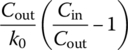 |
||
| 1 |  |
||
| 2 | 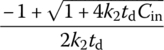 |
 |
|
| Any n | Numerical solution | 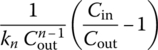 |
Table 6.11 PFR performance at batch or steady state.
| Reaction order, n (r = −kncn) | Cout | td | |
| 0 | |||
| 1 | |||
| 2 |  |
||
| Any n ≠ 1 | 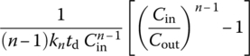 |
Table 6.12 Tracer behavior in a complete mixing reactor and PFR.
| Reactor type | Equation | Notes |
| CMR | 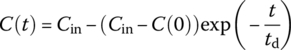 |
Cout at t for system with initial concentration C(0) and steady input of Cin thereafter |
| CMR | 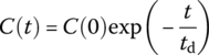 |
Cout at t for system with initial concentration C(0) and Cin = 0 thereaftera |
| PFR | Regardless if input concentration, output is identical, but delayed by td |
a For example, for a spike input at t = 0 and input of clean water thereafter.
6.7 Chemical Kinetics
As one of three pillars of modern reactor design, kinetics quantifies the speed and how the reaction takes place by establishing the reaction mechanism of any reaction. Kinetics can be studied by plotting concentration versus time. Both average and instantaneous time can be used in derivative and integration form. The rate constant identifies these trends based upon different orders of the slope. Rate law is used to determine the different rates based on different starting points and different trends of the reaction rate. Reaction order is found by summation of all the orders to the concentration of each reactant. The derivative of concentration over time equals to the rate constant to the “nth” power (Table 6.13).
Table 6.13 Rate constants and units for n‐th order of chemical reactions
| nth power | k‐function | Rate units |
| 0 | C/t | Moles/seconds |
| 1 | 1/t | 1/seconds |
| 2 | 1/C/t | 1/moles/seconds |
To unveil reaction mechanism, elementary reaction refers to one step in chemical reactions where a bond of a molecule breaks, a bond between atoms is formed, or an electron is transferred. Elementary reactions refer to atoms or molecules. The formation of carbon dioxide through carbon and oxygen gas, for example, is not a elementary reaction. The split of the bond between oxygen gas and its individual addition to carbon is an elementary reaction. Reaction mechanism describes how the bonds are split and created or how the electrons are transferred in the reaction. In most chemical reactions, active intermediates are produced by elementary reactions during a chemical reaction. This transition compound of bonds that have yet to form but is proceeding toward the products is termed as activated complex. For a chemical bond to break or form, activation energy (Ea) should be overcome by the kinetic energy necessary for a reaction to occur. The kinetic energy a molecular possesses is proportional to temperature. Rate determination steps can be understood by the reactants consumed and product produced, where slow reactions have limited steps in reactor design. Pseudo‐first order refers to reactions where the changes in the concentration of other reactant except one are so minimal that they do not represent a real first‐order reaction.
The reaction orders are determined by the rate of reactant disappeared. Reaction orders can be determined by the linear plots according to Table 6.14.
Table 6.14 Linearized kinetic equations.
| Reaction order | Zeroth order | First order | Second order |
| Derivative rate law r = (−dC/dt) | k | kC | kC2 |
| Integrated rate law | C = −kt + C0 | C = C0e−kt | C = 1(kt + 1/C0) |
| Linear equation | C = −kt + C0 | ln C = −kt + ln C0 | 1/C = kt + 1/C0 |
| Linear plots | C vs. t | ln C vs. t | 1/C vs. t |
| Half‐life | C0/(2k) | ln 2/k | 1/(kC0) |
| Units of rate constant k | M time−1 | time−1 | M−1 time−1 |
Half‐life could either be independent of the reactant as a first‐order reaction and only proportional to the rate coefficient or be dependent on the reactant and the rate coefficient as shown in the second‐order reaction. The rate coefficient is dependent on the initial concentration temperature.
In general kinetic analysis, a linear straight line is plotted between properly arranged concentration data against time by either differential or integral methods. Differential method (nth‐order reaction) can be expressed as follows:

Integral method (nth‐order reaction):

For rate forms other than nth‐order, straight‐line relationships are also sought. For example, for Michaelis–Menten rate of a biological process,
The equation could be arranged in a differential form:

and an integral form:
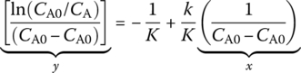
Either forms would yield a straight‐line relationship and could be used to determine reaction kinetics. Elementary reactions are the fundamental steps on how reactions break or form chemical bonds. Collision models consider that the atoms collide with each other to form molecule bonds and to also break old bonds with the correct orientation and sufficient energy. Reaction coordinate diagrams show how the energy changes are processed through a step‐by‐step timeline to see how rearrangement of atoms and molecules occurs. Kinetic energy distribution graphs show that temperature plays a role in how kinetic energy is distributed and used. For example, Maxwell–Boltzmann distribution is used to describe kinetic energy needed for the reaction of the compound. The Arrhenius equation describes the effect of temperature and catalyst on reaction rate for a reaction:
This equation explicitly shows the effect of reactant concentrations on the rate. The effect of temperature and a catalyst on the rate of a reaction is described as the Arrhenius equation, which links the collisions with temperature and energy. The Arrhenius equation indicates that rate constant k depends on temperature. It can be used to determine the value of the activation energy, Ea.
The effect of temperature on rate constants is given quantitatively by the Arrhenius equation:
where
- A is the “frequency factor”
- Ea is the activation energy
- R is the ideal gas constant
- T is the absolute temperature
 is the fraction of molecules whose kinetic energy is equal to or greater than Ea
The value of k increases as the temperature increases and in the presence of a catalyst. The Arrhenius equation can be linearly plotted according to the following equation. Activation energy and concentration could be used to experimentally obtain the activation energy of a reaction, Ea:
where
- T must be in Kelvin
- A is the Arrhenius constant (frequency of successful collisions based on collision geometry and where energy)
- R = 8.314 J/K/mol
- When ln k is plotted against 1/T, the slope = −Ea/R
Table 6.15 Rate constant k and temperature T. Figure 6.8 ln(k) versus 1/T.
Rate constant k (s−1)
Temperature T (°C)
2.88 × 10⁻⁴
320
4.87 × 10⁻⁴
340
7.96 × 10⁻⁴
360
1.26 × 10⁻³
380
1.94 × 10⁻³
400
6.8 Group Theory Predicting Hydroxyl Radical Kinetic Constants
In an advanced oxidation process (AOP), hydroxyl radical reaction holds the key to all oxidation of different organic pollutants (Li and Crittenden, 2009). Since kinetic experiments are costly and time consuming, thermokinetics could be used to theoretically calculate the reaction rate constant k according to the group theory (Minakata and Crittenden, 2011; Minakata et al., 2009, 2011). Benson’s thermochemical group additivity theory hypothesizes that an observed experimental rate constant for a given organic compound is the combined rate of all elementary reactions involving HO•, which can be estimated using Ea. For each reaction mechanism, there is a base activation energy, ![]() , and a functional group contribution of activation energy, EaRi, due to the neighboring (i.e. α‐position) and/or the next‐nearest neighboring (i.e. β‐position) functional group (i.e. Ri). These contributions to the rate constant can be parameterized and determined empirically when sufficient rate constant data are available. Four reaction mechanisms that HO• initiates in the aqueous phase are (i) H‐atom abstraction, (ii) HO• addition to alkenes, (iii) HO• addition to aromatic compounds, and (iv) HO• interaction with sulfur (S)‐, nitrogen (N)‐, or phosphorus (P)‐atom‐containing compounds. Accordingly, an overall reaction rate constant, koverall, may be given in Equation (6.1), where kabs, kadd‐alkene, kadd‐aromatic, and kint are the rate constants for the aforementioned reaction mechanisms. Figure 6.9 shows that linear relationship exists between the Taft constant of a substituent group σ* and the group contribution factor X. Electrophilic substituent σ+ would contribute linearly to the group contribution factor Z (Figure 6.10);
, and a functional group contribution of activation energy, EaRi, due to the neighboring (i.e. α‐position) and/or the next‐nearest neighboring (i.e. β‐position) functional group (i.e. Ri). These contributions to the rate constant can be parameterized and determined empirically when sufficient rate constant data are available. Four reaction mechanisms that HO• initiates in the aqueous phase are (i) H‐atom abstraction, (ii) HO• addition to alkenes, (iii) HO• addition to aromatic compounds, and (iv) HO• interaction with sulfur (S)‐, nitrogen (N)‐, or phosphorus (P)‐atom‐containing compounds. Accordingly, an overall reaction rate constant, koverall, may be given in Equation (6.1), where kabs, kadd‐alkene, kadd‐aromatic, and kint are the rate constants for the aforementioned reaction mechanisms. Figure 6.9 shows that linear relationship exists between the Taft constant of a substituent group σ* and the group contribution factor X. Electrophilic substituent σ+ would contribute linearly to the group contribution factor Z (Figure 6.10);
Figure 6.9 Total of 434 HO reaction rate constant from calibrations and predictions versus experimental rate constants for four reaction mechanism. Error bars represent the range of experimentally reported values. Figure 6.10 Comparison of the group contribution factors for H‐atom abstraction with the Taft constant, σ* (top), and those for HO• addition to aromatic compounds with electrophilic substituent parameter, σ+ (bottom). (Source: Reproduced with permission of American Chemical Society.)

6.9 Photocatalytic Oxidation of Halogen‐substituted Meta‐phenols by UV/TiO2
One of the most important ways to reduce reaction time is through a catalyst. TiO2 has wide applications in oxidation and disinfection of water, wastewater, and volatile organic in air (Hammouda et al., 2017; Tang and An, 1995). In addition, TiO2 is also important for water splitting to produce hydrogen and medical cancer phototherapy. Hole versus hydroxyl radical oxidation is a crucial step toward full comprehension and control of photooxidation processes. Hole oxidation has been reported by much experimental evidence (Meekins and Kamat, 2011; Thompson and Yates, 2005; Zhang and Yates, 2010; and Di Valentin and Fittipaldi, 2013). QSAR was applied by Tang (2011) to probe oxidation mechanisms using UV/TiO2. TiO2 is a typical photocatalyst, which generates hole and hydroxyl radical at different pHs and reduces the oxidation time of organic compounds significantly. Photoexcitation of the semiconductor by photons with energy greater than the band gap will cause electrons (e−) to get excited from the valence band to the conduction band. As a result, positively charged “vacancies,” positive holes (h+), will be left in the valence band:
After the positive holes migrated to the surface of the catalyst, they could oxidize the adsorbed substrates via direct electron transfer if it is thermodynamically favorable:
At the same time, the surface containing holes can generate hydroxyl radicals by oxidizing the adsorbed water and/or hydroxide ions on the TiO2 surface, which in turn can oxidize pollutants at the solid–liquid interface:
Both hydroxyl radical attack and hole oxidation are operative during TiO2 oxidation of organic compounds. However, the competition between the hydroxyl radical attack and direct positive hole oxidation for organics in the process is poorly understood. One of the major difficulties in distinguishing positive hole oxidation versus hydroxyl radical attack is that identical products might be expected from either hydroxyl radical attack or initial hydration of a primary hole‐oxidized cation radicals. In most cases, oxygen is used as electron scavenger, while methanol is typically used as the hole scavenger. For example, the hydroxylation of phenol can proceed either by direct attack by hydroxyl radical, producing a characteristic distribution of hydroxylated isomers, or by primary electron transfer to generate a cation radical. The effect of halogen substituents including F, Cl, and Br at metaposition on the photocatalytic oxidation kinetics at different pH values could shine some light into this controversy issue. For example, the Hammett analysis is used as a tool to probe the electronic effect of halogen substituents on the oxidation kinetics, because the slopes of Hammett plots usually reflect the electronic nature of the transition state complex of the species being oxidized. The pH effect on the Hammett plots is interpreted in terms of when and how these two fundamental oxidation mechanisms are operative under specific experimental conditions.
Langmuir–Hinshelwood (LH) Modeling of the Oxidation Kinetics of Meta‐phenols: The substituent effect on photocatalytic oxidation kinetics of halogen‐substituted phenols is presented here using phenol, which was studied as a reference compound. Figure 6.11 shows the normalized organic concentration remaining versus irradiation time for different initial concentrations of phenol at pH 9. Without illumination, the initial recoveries vary from 92 to 74% after the separation of TiO2 catalyst from the solution. The amount of organic pollutants lost is presumably due to loss by initial adsorption onto the catalyst. The oxidation rate in terms of percentage removal decreases with initial concentration, but the absolute degradation rate increases with higher initial concentrations.

Figure 6.11 Photocatalytic degradation of phenol. Experimental conditions: pH = 3, wavelength = 350 nm, temperature = 42°C, TiO2 = 0.1 g/l.
Experimental conditions: pH = 3, wavelength = 350 nm, temperature = 42°C, TiO2 = 0.1 g/l.
The LH model is used:
where
- ro is the initial oxidation rate dC/dt|t=0 (mM/min)
- Co is the initial concentration of the pollutant (mM)
- k is the oxidation rate constant (mM/min)
- K is the adsorption equilibrium constant onto the catalyst surface (mM−1)
Based upon the LH model, the inverse initial oxidation rate (1/r0) is linearly proportional to the inverse initial concentration (1/C0). The y‐intercept and the slope of the line give 1/k and 1/kK, respectively.
pH Effect on Photocatalytic Oxidation of Halogen‐substituted Meta‐phenols: Figures 6.12 and 6.13 illustrate that the LH kinetics is maintained at pH 3 and 9 with the regression coefficient above 0.95 for each correlation line. From these figures, the adsorption constants and the oxidation constants are obtained at each pH level.
Figure 6.12 Reciprocal initial rate versus reciprocal initial concentration for halogen‐substituted phenols (pH = 3). Experimental conditions: pH = 3, wavelength = 350 nm, temperature = 42°C, TiO2 = 0.1 g/l.
Figure 6.13 Reciprocal initial rate versus reciprocal initial concentration for halogen‐substituted phenols (pH = 9). Experimental conditions: pH = 9, wavelength = 350 nm, temperature = 42°C, TiO2 = 0.1 g/l.
Experimental conditions: pH = 3, wavelength = 350 nm, temperature = 42°C, TiO2 = 0.1 g/l.
Experimental conditions: pH = 9, wavelength = 350 nm, temperature = 42 C, TiO2 = 0.1 g/l.
pH Effects on the Adsorption Constants: Table 6.16 presents the LH adsorption constants of phenol, m‐chlorophenol, m‐bromophenol, and m‐fluorophenol as affected by pH. The adsorption constants for all the substituents except m‐fluorophenol decrease with increasing pH and have the maximum values at pH 3.
Table 6.16 pH effect on the adsorption constants K (mM−1).
| pH | 3 | 5 | 7 | 9 | 11 |
| Phenol | 2.997 | 1.242 | 0.485 | 0.850 | a |
| 3‐Fluorophenol | 0.0172 | 0.084 | 2.430 | 2.890 | a |
| 3‐Chlorophenol | 2.557 | 0.510 | 0.229 | 0.263 | a |
| 3‐Bromophenol | 2.1089 | 0.346 | 0.296 | 3.300 | a |
a Experimental data cannot be described by the Langmuir–Hinshelwood model.
Since the isopotential pH for titanium dioxide is about 6.6 and pKa for substituted phenols is about 8.8, the pH effect on the adsorption typically results from the electrical repulsion between the negatively charged TiO2 surface and the phenolate anions as pH increases. The increasing pH will increase not only the negative charge of TiO2 surface but also the hydroxyl ion concentration competing with the substrates for adsorption sites. As a result, the competitive adsorption between hydroxide ions and phenolate ions may result in minimum oxidation rates at pH near 10, assuming the generation of hydroxyl radicals by adsorbed hydroxyl ions as the rate‐limiting step.
pH Effects on the Oxidation Constants: The pH effect on the oxidation constants of the halogen‐substituted phenols is presented in Table 6.17. When Table 6.17 is compared with Table 6.16, pH has the exactly opposite effect on the oxidation and adsorption constants. In other words, whenever K values reach a maximum for a compound, the k values at that pH level reach a minimum, and vice versa. This suggests that adsorption may not be the determining factor in terms of the oxidation of the halogen‐substituted phenols. Instead, the fundamental mechanisms involved in the photocatalytic oxidation of substituted phenols could be the reason for the observed decoupling trends of the pH effect on oxidation and adsorption constants.
Table 6.17 pH effect on the oxidation rate constants k (mM/min).
| pH | 3 | 5 | 7 | 9 | 11 |
| Phenol | 0.0247 | 0.0388 | 0.0385 | 0.0685 | a |
| 3‐Fluorophenol | 0.1097 | 0.1396 | 0.0237 | 0.032 | a |
| 3‐Chlorophenol | 0.0247 | 0.033 | 0.062 | 0.0984 | a |
| 3‐Bromophenol | 0.033 | 0.0369 | 0.0858 | 0.0196 | a |
a Experimental data cannot be described by the Langmuir–Hinshelwood model,
These results could be understood in terms of the thermodynamic requirements in photocatalytic oxidation of halogen‐substituted phenols. The thermodynamic requirement for direct hole oxidation is that the redox potential of the electron donor, e.g. oxidizable species, should be lower than the valence band gap. For an electron acceptor, e.g. reducible species, the redox potential is greater than that of the conduction band gap. These reactions compete with electron–hole recombination, and their efficiency depends mainly on how fast the charge carriers can reach the surface. The thermodynamic feasibility of these redox reactions can be assessed by considering that the typical redox potentials for many compounds found in an electrolyte like water indeed lie within the band potential of TiO2. If the solution pH decreases, the band gap between valence band and the conduction band could change from 2.2 up to 3.3 eV for anatase TiO2. Therefore, direct oxidation of organic substrates by positive hole will be favored. On the other hand, more hydroxide ion in basic solutions will become the predominant species on catalyst’s surface, and more hydroxyl radicals will be generated. This would favor the hydroxyl radical oxidation of organic compounds.
Different concentrations of potential‐determining adsorbable ions can change the potential drop across the semiconductor/electrolyte interface, thus altering the flat band positions. H+ and OH− ions are potential‐determining ions for metal oxides; thus the electrode potential of the semiconductor changes accord with the following equation:
Therefore, electrons in the conduction band are better reducing agents under basic conditions, while positive holes in the valence band are stronger oxidizers at low pH. Since the conduction band of anatase TiO2 lies at about −3 V (vs. NHE) at pH 0 and roughly −2.2 V at pH 14, the oxidation potentials for water and hydroxide ions remain thermodynamically favorable within all the pH range. The generation of OH. is expected through the following reactions when the potential of a positive hole in a valence band of TiO2 is greater than the following values at pH 7:
OH− is easier to be oxidized by hydroxyl radical than water thermodynamically. However, in acidic pH range, the amount of hydroxide ions is several times less than in the basic solution. As a result, the formation of hydroxyl radicals may be kinetically slow due to significantly less hydroxide ions available in the acidic solution. When all the above factors are taken into consideration, it could be reasonable that positive holes are mostly consumed through the direct oxidation of organic compounds when pH is less than 5. Therefore, the inverse relationship between the adsorption constants and the oxidation rate constants suggests that the reactions at high pH are more dependent upon hydroxyl radical attack, because hydroxyl radicals are generated at the catalyst surface and then diffuse into the bulk solution within a few nanometers to subsequently react with the substrates. This would obviate the need for strong substrate adsorption at higher pH. The faster reaction rates at high pH suggest that reaction via hydroxyl radical attack is faster than via adsorption and subsequent direct electron transfer to positive holes.
The oxidation rate constants of m‐fluorophenol significantly decreased at pH 9 compared with m‐chlorophenol and m‐bromophenol as shown in Table 6.17. Since the fluorine atom is the strongest electron‐withdrawing group, the fluorine substituent will greatly delocalize the π electrons on the aromatic ring. As a result, there is a lower probability for a hydroxyl radical to gain an electron from the aromatic ring during the hydroxylation process. Therefore, the oxidation kinetic pattern of m‐fluorophenol implies that the energy barrier for hydroxyl radicals to attack the aromatic rings of the m‐fluorophenol is much higher than that for m‐chlorophenol and m‐bromophenol. At lower pH, the TiO2 surface is less hydroxylated, so hydroxyl production may be limited. This would make the reaction rely more on the oxidation induced by positive holes, which are also better oxidizers at low pH since the band gap potential is higher. The overall results are the increasing oxidation constants of m‐fluorophenol at pH of 3 and 5.
Hammett Correlations for Halo‐substituted Meta‐phenols: Based on the apparent relationship of the LH kinetic forms, Hammett correlation analysis may further explore the different reaction mechanisms; Table 6.18 lists all the Hammett constants of the related organic compounds.
Table 6.18 Hammett constants for the substituents.
| Substituents | σm | σm+ | F | R |
| F | 0.35 | 0.34 | 0.43 | −0.34 |
| Cl | 0.4 | 0.37 | 0.41 | −0.15 |
| Br | 0.41 | 0.37 | 0.44 | −0.17 |
Electronic Resonance Effect on the Oxidation Rates: At first, log(k/kH) was plotted against σm, but no linear conformity was observed (r2 = 0.5952). Since σm is the Hammett constant that reflects the electronic inductive effect and excludes the resonance effect, the nonlinearity suggests that the electronic inductive effect is minor. Construction of a plot with σm+ constants yielded a good correlation (r2 = 0.947). Therefore, this implies that there is indeed a direct conjugation of the substituent with the reaction center. Since reactions that involve interaction between a substituent and a developing positive charge in the transition state are well correlated with σ+, the correlation suggests that the transition state complex formed during the oxidation very likely has a positive charge. The electronic requirements of photocatalytic oxidation of the metasubstituted phenols can be satisfied by the conjugative interaction between the halogen substituents and the π electrons on the aromatic ring.
The resonance effect has been further verified by even better correlations between log(k/kH) and Swain–Lupton R parameters (r2 = 0.9966), as presented in Figure 6.14. The rather successful correlation with R values implies that there is extensive resonance interaction of the substituents with the π electrons on the aromatic ring. As a result, the resonance effect will stabilize the radical cation by charge delocalization after adsorption and electron transfer to a photo‐generated hole at the TiO2 surface. The sign and magnitude of the slope ρ at pH 3 are −0.4623, which is consistent with the radical cation formation in the rate‐determining step. The negative sign indicates strong electron demand at the reaction site. The data obtained show better linearity (r = 0.97) with σ+ than with σ values (r = 0.83), indicating that direct electron transfer to the photo‐generated hole gives rise to a radical cation. The magnitude of the ρ value (−0.56, r2 = 0.97) was assumed to reflect a near diffusion‐controlled electron transfer to a positive hole, a process that must be preceded by adsorption of the substrate onto the active TiO2.
Figure 6.14 Hammett plot using Swain–Lupton aromatic substituent constant (R) for halogen‐substituted meta‐phenols. Experimental conditions: wavelength = 350 nm, temperature = 42°C, TiO2 = 0.1 g/l.
pH Effects on Hammett Correlations: Figure 6.14 gives further insight into the variations exhibited in the Hammett plots due to increasing pH. By inspection of Figure 6.14, the slopes of Hammett plots at pH 3 and 5 are negative and parallel. This implies that the same reaction process and pathway may be operative at both pH levels, respectively. The negative slopes of the Hammett plots at pH 3 and 5 imply that the transition state complex formed between the substrate and the oxidation species at this pH range is positively charged at the reaction center.
Experimental conditions: Wavelength = 350 nm, temperature = 42°C, TiO2 = 0.1 g/l.
Several factors favor the formation of a positive‐charged transition complex in acidic condition. First, all the halogen‐substituted phenols have higher adsorption density at low pH than at high pH. This favors the direct electron transfer reaction pathway. Second, a positive hole has higher valence band potential in an acidic solution than in a basic solution. Third, a positive hole is a full positive charge while hydroxyl radicals are neutral species. As a mechanistic inference, these Hammett plots suggest that the main degradation pathway may be initiated by direct charge transfer from the organic compound directly to the positive holes at low pH values at 3 and 5. When pH increased from 5 to 7, the negative slope became positive (ρ = +0.6719, r2 = 0.883) due to a sharp reduction in the reactivity of m‐fluorophenol. The small slope at pH 7 is more consistent with a neutral radical process rather than a radical cation intermediate, because the transition state complex would be a neutral radical if hydroxyl radical were the predominant oxidation species. Thus, as pH increases, the reactions are more likely to be an .OH attack than direct electron transfer after adsorption.
Different kinetics and mechanisms of UV/TiO2 suggests that reaction time could change significantly under different reaction conditions.
6.10 Environmental Issues on Different Temporal Scales
Temporal scale could span from product life cycle, human lifetime, to civilization. Within production use at its disposal, life cycle assessment (LCA) is a major tool in quantifying its environmental impacts using software such as LCA2.1 by the US EPA (Bare, 2011). Figure 6.15 illustrates different scopes of environmental concerns with respect to different time horizons such as product, human lifetime, or civilization. Indeed, sustainable development aims to protect the capital of future generations so that mankind can thrive on planet Earth and is in harmony with nature for generations to come.

Figure 6.15 Scopes of environmental versus temporal concerns.
6.10.1 Correlation Between Temporal and Spatial Scales in the Sustainable Design of WTPs and WWTPs
In designing EEIS, there is correlation between spatial and temporal scales. For example, at the molecular level of nanometer, chemical reactions take place within nanoseconds in terms of bond breaking or forming. For particles of less than one millimeter such as colloidal particles, several seconds might be required. A typical example is reaction mechanism of Fenton’s reagent. In 1895, Henry Fenton (Fenton and Jones 1895) reported the color change during hydrogen peroxide oxidation of tartaric acids catalyzed by ferrous ion. Oxygen was thought as the oxidant because the kinetic studies were carried out according to the weight of oxygen releasing from the system. Fifty years later, Haber and Weiss (1934) proposed hydroxyl radical as the dominant oxidative species which initiated the vigorous radical chemistry. While Bray and Gorin (1932) proposed ferrate Fe(IV) as active intermediate in Fenton oxidation. Only after Kremer (2003) confirmed that the formation rate of hydroxyl radical versus ferryl ion is pH dependence. Yamamoto et al. (2012) confirmed that the ferryl−oxo species is the primary oxidizing agent in reactions of Fenton’s reagent because the ferryl−oxo species is more energetically favorable than that yielding a free hydroxyl radical, by 24.4 kcal/mol. For these reasons, chemical reaction mechanisms should be fully understood at different time scales so that the reactions could be accurately scaled up to unit process at several meters scale such as a reactor. Since hydraulic retention time is usually measured in hours, and EEIS requires reliable design on its corresponding temporal scales (Figure 6.16).

Figure 6.16 Time and length multiscales for the sustainable design of WTPs and WWTPs.
Figure 6.17 shows that the correlation of spatial and temporal scales could be further divided into 10−8 to 10−16 m on a spatial scale and 10−8 to 10−16 s on a temporal scale at the molecular/electronic level for a reaction mechanism, which is adopted from Charpentier (2016). How to scale up kinetics to unit process and full plant poses true challenges for the next generation of SEE designers.

Figure 6.17 Organizing the complexity levels on the time and length scales by the integrated multiscale approach for sustainable design of WTPs and WWTPs.
Figure 6.18 illustrates different levels of active research being conducted. Quantum mechanics requests electron, photon, and magnetic effects on innovative technologies, WTPs and WWTPs. For example, vacuum ultraviolet disinfection and oxidation, magnetic destabilization of colloidal particles in water or wastewater, and photocatalytic oxidation of organic pollutants all belong to this group. On a mesoscale, nanotechnologies such as nanocarbon tubes, nano‐TiO2, and oxidized graphene for water treatment have also shown as promising technologies.
Figure 6.18 The scales of modeling and simulation for the sustainable design of WTPs and WWTPs.
Figure 6.19 presents different computation tools for the multiscale modeling of the sustainable design of WTPs and WWTPs. Process system modeling (PSM) can be carried out by specific software such as activated sludge model 3 (ASM3). Computational fluid dynamics (CFD) includes finite volume (FV), finite element (FE), and the lattice Boltzmann (LB) approach. CFD is used extensively in simulating reactor, process, and plants for water and wastewater treatment. Computational chemistry (CCH) includes mesoscale models (MM), microfinite element (microFE), molecular dynamics (MD), and quantum chemistry (QCH).
Figure 6.19 Computational tools in multiscale modeling for sustainable design of WTPs and WWTPs.
6.11 Exercise
6.11.1 Questions
- How is resiliency of EEIS defined and quantified?
- What is an unsteady system, and what is the characteristic of an equation describing an unsteady system?
- What is elementary reaction? Please give one example in water or wastewater treatment for bond breaking, bond forming, or electron transfer reaction add, respectively.
- What is transition state complex?
- What is activation energy?
- How does reaction rate increase with temperature?
- Why are traditional WTPs and WWTPs not efficient?
- Please search and list the major advantages of a static mixer.
6.11.2 Calculation
- Please use group theory and estimate the hydroxylation rate constants of phenol, m‐chlorophenol, m‐bromophenol, and m‐fluorophenol by hydroxyl radical in aqueous solution by using the method developed in the paper by Minakata and Crittenden (2011). Please answer the following:
- Are these the hydroxylation rate constants of metasubstituted chlorophenols by aqueous hydroxyl radicals agreed with literature data? Why or why not?
- How would you rank the degradation rate of these metasubstituted chlorophenols by aqueous hydroxyl radicals?
- Do these ranking orders also agreed with the experimental degradation kinetic rate k presented in Table 6.17 at pH 3 and 9, respectively? Why or why not?
- The following pollutants are listed. Please answer the following questions about their reaction kinetic constants with hydroxyl radical according to Table 6.19:
- Which group has a high‐rate constant reacting with hydroxyl radical? Substituted benzene versus substituted phenol?
- For substituted benzene, please rank the order of rate constant reacting with hydroxyl radical.
Table 6.19 Pollutions and pollution equivalent values.
Pollutants
Pollution equivalent values (kg)
Substituted benzene
Nitrobenzene
0.2
Benzene
0.02
Methylbenzene
0.02
Ethylbenzene
0.02
ortho‐Xylene
0.02
para‐Xylene
0.02
meta‐Xylene
0.02
Chlorobenzene
0.02
ortho‐Dichlorobenzene
0.02
p‐Dichlorobenzene
0.02
p‐Nitrochlorobenzene
0.02
2.4‐Dinitro‐chlorobenzene
0.02
Substituted phenol
Phenol
0.02
m‐Cresol
0.02
2.4‐Dichlorophenol
0.02
2.4.6‐Trichlorophenol
0.02
6.11.3 Project
6.11.3.1 Xiongan Project
Since Xiongan will have a population of 1, 2, and 5 million in 5, 10, and 20 years, respectively, what would be the ratio of peak daily flow/average daily flow of your design for 5, 10, or 20 years? How would these ratios affect the design of WRRFs? Population equivalency determines which technology is the best. According to the population growth, please develop an integrated urban water management plan according to the following principles:
- Water resource, WTP, WWTP, and urban stormwater should be designed with consideration of water cycle and human and ecological demands.
- All the EEIS should be designed for specific purpose not fit for all with stakeholders’ input.
- All the EEIS should be designed, integrated, and interconnected to increase resiliency over 20, 50, and 100 years.
- Please identify top five major factors that would contribute to the uncertainty of the resiliency of different EEIS, respectively.
- Please find a method to quantify the uncertainty of the resiliency of the EEIS using the metric that you selected.
6.11.3.2 Community Proposal Project
Go to the website of your local governmental agency to collect the last 10 years’ population statistics. Is the city of your hometown in a steady or unsteady state in terms of population?
- Discuss which predictive models presented in this chapter you think is the most reliable and why.
- Please predict population growth of the city that you selected in 5, 10, and 20 years.
- Identify three major stressors on water supply, WRRFs, and drainage systems, and rank the resiliency of each EEIS under these stressors.
- Propose design strategies to increase resiliency of each EEIS under each stressor.
Contact your local WWTP manager to obtain the daily flow rate of wastewater, design an equalization tank according to the example, and compare the equalization tank in the local WWTP and make recommendations for improvement, if any.
References
- Bare, J.C., (2011). TRACI 2.0 – the tool for the reduction and assessment of chemical and other environmental impacts. Clean Technologies and Environmental Policy 13 (5): 687–696.
- Bray, W.C. and Gorin, M.H. (1932). Ferryl ion, a compound of tetravalent iron. Journal of American Chemical Society 54: 2124–2125.
- Charpentier, J.C., (2016). What kind of modern “green” chemical engineering is required for the design of the “Factory of Future”? Procedia Engineering 138: 445–458.
- Cuppens, A., Smets, I., and Wyseure, G. (2012). Definition of realistic disturbances as a crucial step during the assessment of resilience of natural wastewater treatment systems. Water Science and Technology 65: 1506–1513.
- Currie, J., Wragg, N., Roberts, C. et al. (2014). Transforming “value engineering” from an art form into a science – process resilience modelling. Water Practice and Technology 9: 104–114.
- Davis, M.L. (2010). Water and Wastewater Engineering: Design Principles and Practice, 1e. New York: McGraw‐Hill Education.
- Di Valentin, C. and Fittipaldi, D. (2013). Hole scavenging by organic adsorbates on the TiO2 surface: a DFT model study. Journal of Physical Chemistry Letters 4 (11): 1901–1906.
- Fenton, H.J. and Jones, H.O. (1895). The oxidation of organic acids in the presence of ferrous iron, Part I. Proceeding of Chemical Society 899–910.
- Francis, R. and Bekera, B. (2014). A metric and frameworks for resilience analysis of engineered and infrastructure systems. Reliability Engineering and System Safety 121: 90–103.
- Goldbloom‐Helzner, D., Opie, J., Pickard, B., and Mikko, M. (2015). Flood resilience: a basic guide for water and wastewater utilities. WEFTEC2015 proceedings, Chicago (26–30 September), pp. 2029–2032.
- Haber, F. and Weiss, J. (1934). The catalytic decomposition of hydrogen peroxide by iron salts. Proceedings of the Royal Society of London, A 147: 332–351.
- Hammouda, S.B., Zhao, F.P., Safaei, Z. et al. (2017). Degradation and mineralization of phenol in aqueous medium by heterogeneous monopersulfate activation on nanostructured cobalt based‐perovskite catalysts ACoO3 (A = La, Ba, Sr and Ce): Characterization, kinetics and mechanism study. Applied Catalysis B: Environmental 215: 60–73.
- Holling, C.S. (1973). Resilience and stability of ecological systems. Annual Review of Ecology, Evolution, and Systematics 4: 1–23.
- Holling, C.S. (1996). Engineering resilience versus ecological resilience. Engineering within Ecological Constraints, pp. 31e43. https://www.nap.edu/catalog/4919/engineering‐within‐ecological‐constraints (accessed 1 March 2017).
- Hwang, H., Forrester, A., and Lansey, K. (2014). Decentralized water reuse: regional water supply system resilience benefits. Procedia Engineering 70: 853–856.
- Juan‐García, P., Butler, D., Comas J.C., Darch, G. et al. (2017). Resilience theory incorporated into urban wastewater systems management: state of the art. Water Research 115: 149–161.
- Kremer, M.L. (2003). The Fenton reaction. Dependence of the rate on pH. Journal of the Physical Chemistry A 107: 1734–1741.
- Lempert, R.J., Groves, D.G., Popper, S.W. et al. (2015). A general, analytic strategies for generating and narrative scenarios. Method Robust 52: 514–528.
- Li, K. and Crittenden, J.C (2009). Computerized pathway elucidation for hydroxyl radical‐induced chain reaction mechanisms in aqueous phase advanced oxidation processes. Environmental Science and Technology 43 (8): 2831–2837.
- Mabrouk, N., Mathias, J.D., and Deffuant, G. (2010). Computing the resilience of a wastewater treatment bioreactor. Proceedings of the 5th International Multi‐conference Computing in the Global Information Technology ICCGI 20e25 (September 2010), pp. 185–188.
- Meekins, B. and Kamat P. (2011). Role of water oxidation catalyst IrO2 in shuttling photogenerated holes across TiO2 interface. Journal of Physical Chemistry Letters 2: 2304–2310.
- Minakata, D. and Crittenden, J. (2011). Linear free energy relationships between aqueous phase hydroxyl radical reaction rate constants and free energy of activation. Environmental Science and Technology 45: 3479–3486.
- Minakata, D., Li, K., Westerhoff, P., and Crittenden, J. (2009). Development of a group contribution method to predict aqueous phase hydroxyl radical (HO•) reaction rate constants. Environmental Science and Technology 43: 6220–6227.
- Minakata, D., Song, W.H., and Crittenden, J. (2011). Reactivity of aqueous phase hydroxyl radical with halogenated carboxylate anions: experimental and theoretical studies. Environmental Science and Technology 45: 6057–6065.
- Mugume, S., Gomez, D., and Butler, D. (2014). Quantifying the resilience of urban drainage systems using a hydraulic performance assessment approach. 13th International Conference on Urban Drainage, Sarawak, Malaysia (7–12 September).
- Radcliffe, J.C. (2015). Water recycling in Australia – during and after the drought. Environmental Science: Water Research and Technology 1: 554–562.
- Schoen, M., Hawkins, T., Xue, X. et al. (2015). Technologic resilience assessment of coastal community water and wastewater service options. Sustainability of Water Quality and Ecology 6: 1–13.
- Sweetapple, C., Fu, G., and Butler, D. (2016). Reliable, robust, and resilient system design framework with application to wastewater‐treatment plant control. American Society of Civil Engineering 1–10. 10.1061/(ASCE)EE.1943‐7870.0001171, 04016086.
- Tang, W.Z. (2011). Photocatalytic oxidation of halogen substituted meta‐phenols by UV/TiO2 in acidic and basic aqueous solutions. Finish Conference of Environmental Science, Turku, Finland (5–6 May 2011).
- Tang, W.Z. and An, H. (1995). UV/TiO2 photocatalytic oxidation of commercial dyes in aqueous solutions. Chemosphere 31 (9): 4157–4170.
- Thompson, T. and Yates, J. (2005). Monitoring hole trapping in photo‐excited TiO2 using a surface photoreaction. Journal of Physical Chemistry B 109: 18230–18236.
- Walker, B., Holling, C.S., Carpenter, S.R., and Kinzig, A. (2004). Resilience, adaptability and transformability in social–ecological systems. Ecology and Society 9 (2): 5.
- Weirich, S.R., Silverstein, J., and Rajagopalan, B. (2015). Resilience of secondary wastewater treatment plants: prior performance is predictive of future process failure and recovery time. Environmental Engineering Science 32: 222–231.
- Xue, X., Schoen, M.E., Ma, X.C. et al. (2015). Critical insights for a sustainability framework to address integrated community water services: technical metrics and approaches. Water Research 77: 155–169.
- Yamamoto, N., Koga, N., and Nagaoka, M. (2012). Ferryl−oxo species produced from Fenton’s reagent via a two‐step pathway: minimum free‐energy path analysis. Journal of Physical Chemistry B 116: 14178−14182.
- Zhang, Z. and Yates, J. (2010). Direct observation of surface‐mediated electron‐hole pair recombination in TiO2. Journal of Physical Chemistry C 114: 3098–3101.