Chapter 3. Topology design

This chapter covers

• Decomposing a problem to fit Storm constructs
• Working with unreliable data sources
• Integrating with external services and data stores
• Understanding parallelism within a Storm topology
• Following best practices for topology design

In the previous chapter, we got our feet wet by building a simple topology that counts commits made to a GitHub project. We broke it down into Storm’s two primary components—spouts and bolts—but we didn’t concern ourselves with details as to why. This chapter expands on those basic Storm concepts by showing you how to think about modeling and designing solutions with Storm. You’ll learn strategies for problem analysis that can help you end up with a good design: a model for representing the workflow of the problem at hand.

In addition, it’s important that you learn how scalability (or parallelization of units of work) is built into Storm because that affects the approach that you’ll take with topology design. We’ll also explore strategies for gaining the most out of your topology in terms of speed.

After reading this chapter, not only will you be able to easily take apart a problem and see how it fits within Storm, but you’ll also be able to determine whether Storm is the right solution for tackling that problem. This chapter will give you a solid understanding of topology design so that you can envision solutions to big data problems.

Let’s get started by exploring how you can approach topology design and then get into breaking down a real-world scenario using the steps we’ve outlined.

3.1. Approaching topology design

The approach to topology design can be broken down into the following five steps:

1. Defining the problem/forming a conceptual solution— This step serves to provide a clear understanding of the problem being tackled. It also serves as a place to document the requirements to be placed on any potential solution (including requirements with regard to speed, which is a common criterion in big data problems). This step involves modeling a solution (not an implementation) that addresses the core need(s) of the problem.
2. Mapping the solution to Storm— In this step, you follow a set of tenets for breaking down the proposed solution in a manner that allows you to envision how it will map to Storm primitives (aka Storm concepts). At this stage, you’ll come up with a design for your topology. This design will be tuned and adjusted as needed in the following steps.
3. Implementing the initial solution— Each of the components will be implemented at this point.
4. Scaling the topology— In this step, you’ll turn the knobs that Storm provides for you to run this topology at scale.
5. Tuning based on observations— Finally, you’ll adjust the topology based on observed behavior once it’s running. This step may involve additional tuning for achieving scale as well as design changes that may be warranted for efficiency.

Let’s apply these steps to a real-world problem to show how you’d go about completing each of the steps. We’ll do this with a social heat map, which encapsulates several challenging topics related to topology design.

3.2. Problem definition: a social heat map

Imagine this scenario: it’s Saturday night and you’re out drinking at a bar, enjoying the good life with your friends. You’re finishing your third drink and you’re starting to feel like you need a change of scene. Maybe switch it up and go to a different bar? So many choices—how do you even choose? Being a socialite, of course you’d want to end up in the bar that’s most popular. You don’t want to go somewhere that was voted best in your neighborhood glossy magazine. That was so last week. You want to be where the action is right now, not last week, not even last hour. You are the trendsetter. You have a responsibility to show your friends a good time.

Okay, maybe that’s not you. But does that represent the average social network user? Now what can we do to help this person? If we can represent the answer this person is looking for in a graphical form factor, it’d be ideal—a map that identifies the neighborhoods with highest density of activity in bars as hot zones can convey everything quickly. A heat map can identify the general neighborhood in a big city like New York or San Francisco, and generally when a picking a popular bar, it’s better to have a few choices within close proximity to one another, just in case.

We’ve provided a general problem definition. Before moving any further, let’s form a conceptual solution.

3.2.1. Formation of a conceptual solution

Where should we begin? Multiple social networks incorporate the concept of check-ins. Let’s say we have access to a data fire hose that collects check-ins for bars from all of these networks. This fire hose will emit a bar’s address for every check-in. This gives us a starting point, but it’s also good to have an end goal in mind. Let’s say that our end goal is a geographical map with a heat map overlay identifying neighborhoods with the most popular bars. Figure 3.1 illustrates our proposed solution where we’ll transform multiple check-ins from different venues to be shown in a heat map.

Figure 3.1. Using check-ins to build a heat map of bars

The solution that we need to model within Storm becomes the method of transforming (or aggregating) check-ins into a data set that can be depicted on a heat map.

3.3. Precepts for mapping the solution to Storm

The best way to start is to contemplate the nature of data flowing through this system. When we better understand the peculiarities contained within the data stream, we can become more attuned to requirements that can be placed on this system realistically.

3.3.1. Consider the requirements imposed by the data stream

We have a fire hose emitting addresses of bars for each check-in. But this stream of check-ins doesn’t reliably represent every single user who went to a bar. A check-in isn’t equivalent to a physical presence at a location. It’s better to think of it as a sampling of real life because not every single user checks in. But that leads us to question whether check-in data is even useful for solving this problem. For this example, we can safely assume that check-ins at bars are proportional to people at those locations.

So we know the following:

• Check-ins are a sampling of real-life scenarios, but they’re not complete.
• They’re proportionately representative.

Note

Let’s make the assumption here that the data volume is large enough to compensate for data loss and that any data loss is intermittent and not sustained long enough to cause a noticeable disruption in service. These assumptions help us portray a case of working with an unreliable data source.

We have our first insight about our data stream: a proportionately representative but possibly incomplete stream of check-ins. What’s next? We know our users want to be notified about the latest trends in activity as soon as possible. In other words, we have a strict speed requirement: get the results to the user as quickly as possible because the value of data diminishes with time.

What emerges from consideration of the data stream is that we don’t need to worry too much about data loss. We can come to this conclusion because we know that our incoming data set is incomplete, so accuracy down to some arbitrary, minute degree of precision isn’t necessary. But it’s proportionately representative and that’s good enough for determining popularity. Combine this with the requirement of speed and we know that as long as we get recent data quickly to our users, they’ll be happy. Even if data loss occurs, the past results will be replaced soon.

This scenario maps directly to the idea of working with an unreliable data source in Storm. With an unreliable data source, you don’t have the ability to retry a failed operation; the data source may not have the ability to replay a data point. In our case, we’re sampling real life by way of check-ins and that mimics the availability of an incomplete data set.

In contrast, there may be cases where you work with a reliable data source—one that has the ability to replay data points that fail. But perhaps accuracy is less important than speed and you may not want to take advantage of the replayability of a reliable data source. Then approximations can be just as acceptable, and you’re treating the reliable data source as if it was unreliable by choosing to ignore any reliability measures it provides.

Note

We’ll cover reliable data sources along with fault tolerance in chapter 4.

Having defined the source of the data, the next step is to identify how the individual data points will flow through our proposed solution. We’ll explore this topic next.

3.3.2. Represent data points as tuples

Our next step is to identify the individual data points that flow through this stream. It’s easy to accomplish this by considering the beginning and end. We begin with a series of data points composed of street addresses of bars with activity. We’ll also need to know the time the check-in occurred. So our input data point can be represented as follows:

[time="9:00:07 PM", address="287 Hudson St New York NY 10013"]

That’s the time and an address where the check-in happened. This would be our input tuple that’s emitted by the spout. As you’ll recall from chapter 2, a tuple is a Storm primitive for representing a data point and a spout is a source of a stream of tuples.

We have the end goal of building a heat map with the latest activity at bars. So we need to end up with data points representing timely coordinates on a map. We can attach a time interval (say 9:00:00 PM to 9:00:15 PM, if we want 15-second increments) to a set of coordinates that occurred within that interval. Then at the point of display within the heat map, we can pick the latest available time interval. Coordinates on a map can be expressed by way of latitude and longitude (say, 40.7142° N, 74.0064° W for New York, NY). It’s standard form to represent 40.7142° N, 74.0064° W as (40.7142, -74.0064). But there might be multiple coordinates representing multiple check-ins within a time window. So we need a list of coordinates for a time interval. Then our end data point starts to look like this:

[time-interval="9:00:00 PM to 9:00:15 PM",
 hotzones=List((40.719908,-73.987277),(40.72612,-74.001396))]

That’s an end data point containing a time interval and two corresponding check-ins at two different bars.

What if there’s two or more check-ins at the same bar within that time interval? Then that coordinate will be duplicated. How would we handle that? One option is to keep counts of occurrences within that time window for that coordinate. This involves determining sameness of coordinates based on some arbitrary but useful degree of precision. To avoid all that, let’s keep duplicates of any coordinate within a time interval with multiple check-ins. By adding multiples of the same coordinates to a heat map, we can let the map generator make use of multiple occurrences as a level of hotness (rather than using occurrence count for that purpose).

Our end data point will look like this:

[time-interval="9:00:00 PM to 9:00:15 PM",
 hotzones=List((40.719908,-73.987277),
               (40.72612,-74.001396),
               (40.719908,-73.987277))]

Note that the first coordinate is duplicated. This is our end tuple that will be served up in the form of a heat map. Having a list of coordinates grouped by a time interval has these advantages:

• Allows us to easily build a heat map by using the Google Maps API. We can do this by adding a heat map overlay on top of a regular Google Map.
• Let us go back in time to any particular time interval and see the heat map for that point in time.

Having the input data points and final data points is only part of the picture; we still need to identify how we get from point A to point B.

3.3.3. Steps for determining the topology composition

Our approach for designing a Storm topology can be broken down into three steps:

1. Determine the input data points and how they can be represented as tuples.
2. Determine the final data points needed to solve the problem and how they can be represented as tuples.
3. Bridge the gap between the input tuples and the final tuples by creating a series of operations that transform them.

We already know our input and desired output:

Input tuples:

[time="9:00:07 PM", address="287 Hudson St New York NY 10013"]

End tuples:

[time-interval="9:00:00 PM to 9:00:15 PM",
 hotzones=List((40.719908,-73.987277),
               (40.72612,-74.001396),
               (40.719908,-73.987277))]

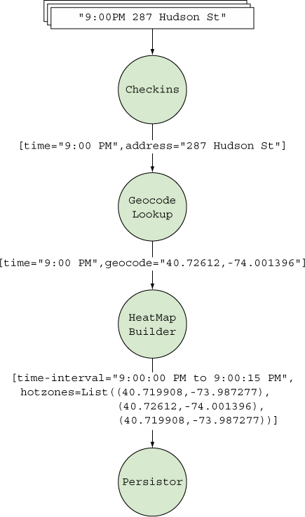
Somewhere along the way, we need to transform the addresses of bars into these end tuples. Figure 3.2 shows how we can break down the problem into these series of operations.

Figure 3.2. Transforming input tuples to end tuples via a series of operations

Let’s take these steps and see how they map onto Storm primitives (we’re using the terms Storm primitives and Storm concepts interchangeably).

Operations as spouts and bolts

We’ve created a series of operations to transform input tuples to end tuples. Let’s see how these four operations map to Storm primitives:

• Checkins— This will be the source of input tuples into the topology, so in terms of Storm concepts this will be our spout. In this case, because we’re using an unreliable data source, we’ll build a spout that has no capability of retrying failures. We’ll get into retrying failures in chapter 4.
• GeocodeLookup— This will take our input tuple and convert the street address to a geocoordinate by querying the Google Maps Geocoding API. This is the first bolt in the topology.
• HeatMapBuilder— This is the second bolt in the topology, and it’ll keep a data structure in memory to map each incoming tuple to a time interval, thereby grouping check-ins by time interval. When each time interval is completely passed, it’ll emit the list of coordinates associated with that time interval.
• Persistor— We’ll use this third and final bolt in our topology to save our end tuples to a database.

Figure 3.3 provides an illustration of the design mapped to Storm concepts.

Figure 3.3. Heat map design mapped to Storm concepts

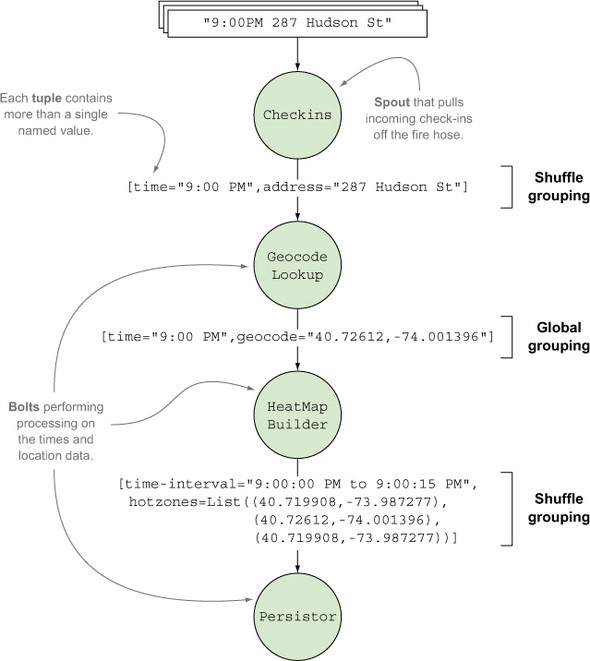
So far we’ve discussed the tuples, spout, and bolts. One thing in figure 3.3 that we haven’t talked about is the stream grouping for each stream. We’ll get into each grouping in more detail when we cover the code for the topology in the next section.

3.4. Initial implementation of the design

With the design complete, we’re ready to tackle the implementation for each of the components. Much as we did in chapter 2, we’ll start with the code for the spout and bolts, and finish with the code that wires it all together. Later we’ll adjust each of these implementations for efficiency or to address some of their shortcomings.

3.4.1. Spout: read data from a source

In our design, the spout listens to a fire hose of social check-ins and emits a tuple for each individual check-in. Figure 3.4 provides a reminder of where we are in our topology design.

Figure 3.4. The spout listens to the fire hose of social check-ins and emits a tuple for each check-in.

For the purpose of this chapter, we’ll use a text file as our source of data for check-ins. To feed this data set into our Storm topology, we need to write a spout that reads from this file and emits a tuple for each line. The file, checkins.txt, will live next to the class for our spout and contain a list of check-ins in the expected format (see the following listing).

Listing 3.1. An excerpt from our simple data source, checkins.txt

1382904793783, 287 Hudson St New York NY 10013
1382904793784, 155 Varick St New York NY 10013
1382904793785, 222 W Houston St New York NY 10013
1382904793786, 5 Spring St New York NY 10013
1382904793787, 148 West 4th St New York NY 10013

The next listing shows the spout implementation that reads from this file of check-ins. Because our input tuple is a time and address, we’ll represent the time as a Long (millisecond-level Unix timestamp) and the address as a String, with the two separated by a comma in our text file.

Listing 3.2. Checkins.java

Because we’re treating this as an unreliable data source, the spout remains simple; it doesn’t need to keep track of which tuples failed and which ones succeeded in order to provide fault tolerance. Not only does that simplify the spout implementation, it also removes quite a bit of bookkeeping that Storm needs to do internally and speeds things up. When fault tolerance isn’t necessary and we can define a service-level agreement (SLA) that allows us to discard data at will, an unreliable data source can be beneficial. It’s easier to maintain and provides fewer points of failure.

3.4.2. Bolt: connect to an external service

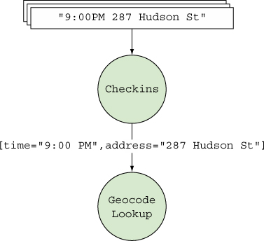
The first bolt in the topology will take the address data point from the tuple emitted by the Checkins spout and translate that address into a coordinate by querying the Google Maps Geocoding Service. Figure 3.5 highlights the bolt we’re currently implementing.

Figure 3.5. The geocode lookup bolt accepts a social check-in and retrieves the coordinates associated with that check-in.

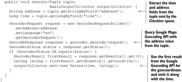
The code for this bolt can be seen in listing 3.3. We’re using the Google Geocoder Java API from https://code.google.com/p/geocoder-java/ to retrieve the coordinates.

Listing 3.3. GeocodeLookup.java

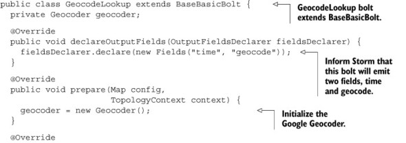
We’ve intentionally kept our interaction with Google Geocoding API simple. In a real implementation we should be handling for error cases when addresses may not be valid. Additionally, the Google Geocoding API imposes a quota when used in this way that’s quite small and not practical for big data applications. For a big data application like this, you’d need to obtain an access level with a higher quota from Google if you wanted to use them as a provider for Geocoding. Other approaches to consider include locally caching geocoding results within your data center to avoid making unnecessary invocations to Google’s API.

We now have the time and geocoordinate of every check-in. We took our input tuple

[time="9:00:07 PM", address="287 Hudson St New York NY 10013"]

and transformed it into this:

[time="9:00 PM", geocode="40.72612,-74.001396"]

This new tuple will then be sent to the bolt that maintains groups of check-ins by time interval, which we’ll look at now.

3.4.3. Bolt: collect data in-memory

Next, we’ll build the data structure that represents the heat map. Figure 3.6 illustrates our location in the design.

Figure 3.6. The heat map builder bolt accepts a tuple with time and geocode and emits a tuple containing a time interval and a list of geocodes.

What kind of data structure is suitable here? We have tuples coming into this bolt from the previous GeocodeLookup bolt in the form of [time="9:00 PM", geocode= "40.72612,-74.001396"]. We need to group these by time intervals—let’s say 15-second intervals because we want to display a new heat map every 15 seconds. Our end tuples need to be in the form of [time-interval="9:00:00 PM to 9:00:15 PM", hotzones= List((40.719908,-73.987277),(40.72612,-74.001396),(40.719908,-73.987277))].

To group geocoordinates by time interval, let’s maintain a data structure in memory and collect incoming tuples into that data structure isolated by time interval. We can model this as a map:

Map<Long, List<LatLng>> heatmaps;

This map is keyed by the time that starts our interval. We can omit the end of the time interval because each interval is of the same length. The value will be the list of coordinates that fall into that time interval (including duplicates—duplicates or coordinates in closer proximity would indicate a hot zone or intensity on the heat map).

Let’s start building the heat map in three steps:

1. Collect incoming tuples into an in-memory map.
2. Configure this bolt to receive a signal at a given frequency.
3. Emit the aggregated heat map for elapsed time intervals to the Persistor bolt for saving to a database.

Let’s look at each step individually, and then we can put everything together, starting with the next listing.

Listing 3.4. HeatMapBuilder.java: step 1, collecting incoming tuples into an in-memory map

The absolute time interval the incoming tuple falls into is selected by taking the check-in time and dividing it by the length of the interval—in this case, 15 seconds. For example, if check-in time is 9:00:07.535 PM, then it should fall into the time interval 9:00:00.000–9:00:15.000 PM. What we’re extracting here is the beginning of that time interval, which is 9:00:00.000 PM.

Now that we’re collecting all the tuples into a heat map, we need to periodically inspect it and emit the coordinates from completed time intervals so that they can be persisted into a data store by the next bolt.

Tick tuples

Sometimes you need to trigger an action periodically, such as aggregating a batch of data or flushing some writes to a database. Storm has a feature called tick tuples to handle this eventuality. Tick tuples can be configured to be received at a user-defined frequency and when configured, the execute method on the bolt will receive the tick tuple at the given frequency. You need to inspect the tuple to determine whether it’s one of these system-emitted tick tuples or whether it’s a normal tuple. Normal tuples within a topology will flow through the default stream, whereas tick tuples are flowing through a system tick stream, making them easily identifiable. The following listing shows the code for configuring and handling tick tuples in the HeatMapBuilder bolt.

Listing 3.5. HeatMapBuilder.java: step 2, configuring to receive a signal at a given frequency

Looking at the code in listing 3.5, you’ll notice that tick tuples are configured at the bolt level, as demonstrated by the getComponentConfiguration implementation. The tick tuple in question will only be sent to instances of this bolt.

Now let’s use that tick tuple as a signal to select time periods that have passed for which we no longer expect any incoming coordinates, and emit them from this bolt so that the next bolt down the line can take them on (see the next listing).

Listing 3.6. HeatMapBuilder.java: step 3, emitting the aggregated HeatMap for elapsed time intervals

Steps 1, 2, and 3 provide a complete HeatMapBuilder implementation, showing how you can maintain state with an in-memory map and also how you can use Storm’s built-in tick tuple to emit a tuple at particular time intervals. With this implementation complete, let’s move on to persisting the results of the tuples emitted by HeatMapBuilder.

3.4.4. Bolt: persisting to a data store

We have the end tuples that represent a heat map. At this point, we’re ready to persist that data to some data store. Our JavaScript-based web application can read the heat map values from this data store and interact with the Google Maps API to build a geographical visualization from these calculated values. Figure 3.7 illustrates the final bolt in our design.

Figure 3.7. The Persistor bolt accepts a tuple with a time interval and a list of geocodes and persists that data to a data store.

Because we’re storing and accessing heat maps based on time interval, it makes sense to use a key-value data model for storage. For this case study, we’ll use Redis, but any data store that supports the key-value model will suffice (such as Membase, Memcached, or Riak). We’ll store the heat maps keyed by time interval with the heat map itself as a JSON representation of the list of coordinates. We’ll use Jedis as a Java client for Redis and the Jackson JSON library for converting the heat map to JSON.

So let’s take a look at the code for writing to this NoSQL data store (see the following listing).

Listing 3.7. Persistor.java

Working with Redis is simple, and it serves as a good store for our use case. But for larger-scale applications and data sets, a different data store may be necessary. One thing to note is that because we’re working with an unreliable data stream, we’re simply logging any errors that may occur while saving to the database. Some errors may be able to be retried (say, a timeout), and when working with a reliable data stream, we’d consider how to retry them, as you’ll see in chapter 4.

3.4.5. Defining stream groupings between the components

In chapter 2, you learned two ways of connecting components within a topology to one another—shuffle grouping and fields grouping. To recap:

• You use shuffle grouping to distribute outgoing tuples from one component to the next in a manner that’s random but evenly spread out.
• You use fields grouping when you want to ensure tuples with the same values for a selected set of fields always go to the same instance of the next bolt.

A shuffle grouping should suffice for the streams between Checkins/GeocodeLookup and HeatMapBuilder/Persistor.

But we need to send the entire stream of outgoing tuples from the GeocodeLookup bolt to the HeatMapBuilder bolt. If different tuples from GeocodeLookup end up going to different instances of HeatMapBuilder, then we won’t be able to group them into time intervals because they’ll be spread out among different instances of HeatMapBuilder. This is where global grouping comes in. Global grouping will ensure that the entire stream of tuples will go to one specific instance of HeatMapBuilder. Specifically, the entire stream will go to the instance of HeatMapBuilder with the lowest task ID (an ID assigned internally by Storm). Now we have every tuple in one place and we can easily determine which time interval any tuple falls into and group them into their corresponding time intervals.

Note

Instead of using a global grouping you could have a single instance of the HeatMapBuilder bolt with a shuffle grouping. This will also guarantee that everything goes to the same HeatMapBuilder instance, as there is only one. But we favor being explicit in our code, and using a global grouping clearly conveys the desired behavior here. A global grouping is also slightly cheaper, as it doesn’t have to pick a random instance to emit to as in a shuffle grouping.

Let’s take a look at how we’d define these stream groupings in the code for building and running our topology.

3.4.6. Building a topology for running in local cluster mode

We’re almost done. We just need to wire everything together and run the topology in local cluster mode, just like we did in chapter 2. But in this chapter, we’re going to deviate from having all the code in a single LocalTopologyRunner class and split the code into two classes: one class for building the topology and another for running it. This is a common practice and while you might not see the benefits immediately in this chapter, hopefully in chapters 4 and 5 you’ll see why we’ve decided to do this.

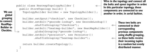
The following listing shows you the code for building the topology.

Listing 3.8. HeatmapTopologyBuilder.java

With the code for building the topology defined, the next listing shows how to implement LocalTopologyRunner.

Listing 3.9. LocalTopologyRunner.java

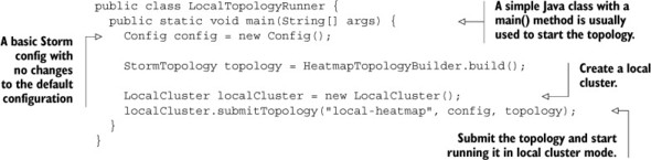
Now we have a working topology. We read check-in data from our spout, and in the end, we persist the coordinates grouped by time intervals into Redis and complete the heat map topology implementation. All we have left to do is read the data from Redis using a JavaScript application and use the heat map overlay feature of the Google Maps API to build the visualization.

This simple implementation will run, but will it scale? Will it be fast enough? Let’s do some digging and find out.

3.5. Scaling the topology

Let’s review where we are so far. We have a working topology for our service that looks similar to the one shown in figure 3.8.

Figure 3.8. Heat map topology

There are problems with it. As it stands right now, this topology operates in a serial fashion, processing one check-in at a time. That isn’t web-scale—that’s Apple IIe scale. If we were to put this live, everything would back up and we would end up with unhappy customers, an unhappy ops team, and probably unhappy investors.

We need to process multiple check-ins at a time, so we’ll introduce parallelism into our topology. One property that makes Storm so alluring is how easy it is to parallelize workflows such as our heat map. Let’s take a look at the parts of the topology again and discuss how they can be parallelized. We’ll begin with check-ins.

3.5.1. Understanding parallelism in Storm

Storm has additional primitives that serve as knobs for tuning how it can scale. If you don’t touch them, the topology can still work, but all components will run in a more or less linear fashion. This may be fine for topologies that only have a small stream of data flowing through them. For something like the heat map topology that’ll receive data from a large fire hose, we would want to address the bottlenecks in it. In this section, we’ll look at two of the primitives that deal with scaling. There are additional primitives for scaling that we’ll consider later in the next chapter.

Parallelism hints

We know we’re going to need to process many check-ins rapidly, so we want to parallelize the spout that handles check-ins. Figure 3.9 gives you an idea of what part of the topology we’re working on here.

Figure 3.9. Focusing our parallelization changes on the Checkins spout

Storm allows you to provide a parallelism hint when you define any spouts or bolts. In code, this would involve transforming

builder.setSpout("checkins", new Checkins());

to

builder.setSpout("checkins", new Checkins(), 4);

The additional parameter we provide to setSpout is the parallelism hint. That’s a bit of a mouthful: parallelism hint. So what is a parallelism hint? For right now, let’s say that the parallelism hint tells Storm how many check-in spouts to create. In our example, this results in four spout instances being created. There’s more to it than that, but we’ll get to that in a bit.

Now when we run our topology, we should be able to process check-ins four times as fast—except simply introducing more spouts and bolts into our topology isn’t enough. Parallelism in a topology is about both input and output. The Checkins spout can now process more check-ins at a time, but the GeocodeLookup bolt is still being handled serially. Simultaneously passing four check-ins to a single GeocodeLookup instance isn’t going to work out well. Figure 3.10 illustrates the problem we’ve created.

Figure 3.10. Four Checkins instances emitting tuples to one GeocodeLookup instance results in the GeocodeLookup instance being a bottleneck.

Right now, what we have is akin to a circus clown car routine where many clowns all try to simultaneously pile into a car through the same door. This bottleneck needs to be resolved; let’s try parallelizing the geocode lookup bolt as well. We could just parallelize the geocode bolt in the same way we did check-ins. Going from this

builder.setBolt("geocode-lookup", new GeocodeLookup());

to this

builder.setBolt("geocode-lookup", new GeocodeLookup(), 4);

will certainly help. Now we have one GeocodeLookup instance for each Checkins instance. But GeocodeLookup is going to take a lot longer than receiving a check-in and handing it off to our bolt. So perhaps we can do something more like this:

builder.setBolt("geocode-lookup", new GeocodeLookup(), 8);

Now if GeocodeLookup takes two times as long as check-in handling, tuples should continue to flow through our system smoothly, resulting in figure 3.11.

Figure 3.11. Four Checkins instances emitting tuples to eight GeocodeLookup instances

We’re making progress here, but there’s something else to think about: what happens as our service becomes more popular? We’re going to need to be able to continue to scale to keep pace with our ever expanding traffic without taking our application offline, or at least not taking it offline very often. Luckily Storm provides a way to do that. We loosely defined the parallelism hint earlier but said there was a little more to it. Well, here we are. That parallelism hint maps into two Storm concepts we haven’t covered yet: executors and tasks.

Executors and tasks

So what are executors and tasks? Truly understanding the answer to this question requires deeper knowledge of a Storm cluster and its various parts. Although we won’t learn any details about a Storm cluster until chapter 5, we can provide you with a sneak peek into certain parts of a Storm cluster that’ll help you understand what executors and tasks are for the purpose of scaling our topology.

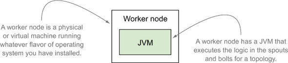
So far, we know that our spouts and bolts are each running as one or more instances. Each of these instances is running somewhere, right? There has to be some machine (physical or virtual) that’s actually executing our components. We’ll call this machine a worker node, and though a worker node isn’t the only type of node running on a Storm cluster, it is the node that executes the logic in our spouts and bolts. And because Storm runs on the JVM, each of these worker nodes is executing our spouts and bolts on a JVM. Figure 3.12 shows what we have so far.

Figure 3.12. A worker node is a physical or virtual machine that’s running a JVM, which executes the logic in the spouts and bolts.

There’s a little more to a worker node, but what’s important for now is that you understand that it runs the JVM that executes our spout and bolt instances. So we pose the question again: what are executors and tasks? Executors are a thread of execution on the JVM, and tasks are the instances of our spouts and bolts running within a thread of execution. Figure 3.13 illustrates this relationship.

Figure 3.13. Executors (threads) and tasks (instances of spouts/bolts) run on a JVM.

It’s really that simple. An executor is a thread of execution within a JVM. A task is an instance of a spout or bolt running within that thread of execution. When discussing scalability in this chapter, we’re referring to changing the number of executors and tasks. Storm provides additional ways to scale by changing the number of worker nodes and JVMs, but we’re saving those for chapters 6 and 7.

Let’s go back to our code and revisit what this means in terms of parallelism hints. Setting the parallelism hint to 8, as we did with GeocodeLookup, is telling Storm to create eight executors (threads) and run eight tasks (instances) of GeocodeLookup. This is seen with the following code:

builder.setBolt("geocode-lookup", new GeocodeLookup(), 8)

By default, the parallelism hint is setting both the number of executors and tasks to the same value. We can override the number of tasks with the setNumTasks() method as follows:

builder.setBolt("geocode-lookup", new GeocodeLookup(), 8).setNumTasks(8)

Why provide the ability to set the number of tasks to something different than the number of executors? Before we answer this question, let’s take a step back and revisit how we got here. We were talking about how we’ll want to scale our heat map in the future without taking it offline. What’s the easiest way to do this? The answer: increase the parallelism. Fortunately, Storm provides a useful feature that allows us to increase the parallelism of a running topology by dynamically increasing the number of executors (threads). You’ll learn more on how this is done in chapter 6.

What does this mean for our GeocodeLookup bolt with eight instances being run across eight threads? Well, each of those instances will spend most of its time waiting on network I/O. We suspect that this means GeocodeLookup is going to be a source of contention in the future and will need to be scaled up. We can allow for this possibility with

builder.setBolt("geocode-lookup", new GeocodeLookup(), 8).setNumTasks(64)

Now we have 64 tasks (instances) of GeocodeLookup running across eight executors (threads). As we need to increase the parallelism of GeocodeLookup, we can keep increasing the number of executors up to a maximum of 64 without stopping our topology. We repeat: without stopping the topology. As we mentioned earlier, we’ll get into the details of how to do this in a later chapter, but the key point to understand here is that the number of executors (threads) can be dynamically changed in a running topology.

Storm breaks parallelism down into two distinct concepts of executors and tasks to deal with situations like we have with our GeocodeLookup bolt. To illustrate why, let’s go back to the definition of a fields grouping:

A fields grouping is a type of stream grouping where tuples with the same value for a particular field name are always emitted to the same instance of a bolt.

Within that definition lurks our answer. Fields groupings work by consistently hashing tuples across a set number of bolts. To keep keys with the same value going to the same bolt, the number of bolts can’t change. If it did, tuples would start going to different bolts. That would defeat the purpose of what we were trying to accomplish with a fields grouping.

It was easy to configure the executors and tasks on the Checkins spout and GeocodeLookup bolt in order to scale them at a later point in time. Sometimes, though, parts of our design won’t work well for scaling. Let’s look at that next.

3.5.2. Adjusting the topology to address bottlenecks inherent within design

HeatMapBuilder is up next. Earlier we hit a bottleneck on GeocodeLookup when we increased the parallelism hint on the Checkins spout. But we were able to address this easily by increasing the parallelism on the GeocodeLookup bolt accordingly. We can’t do that here. It doesn’t make sense to increase the parallelism on HeatMapBuilder as it’s connected to the previous bolt using global grouping. Because global grouping dictates that every tuple goes to one specific instance of HeatMapBuilder, increasing parallelism on it doesn’t have any effect; only one instance will be actively working on the stream. There’s a bottleneck that’s inherent in the design of our topology.

This is the downside of using global grouping. With global grouping, we’re trading our ability to scale and introducing an intentional bottleneck with being able to see the entire stream of tuples in one specific bolt instance.

So what can we do? Is there no way we can parallelize this step in our topology? If we can’t parallelize this bolt, it makes little sense to parallelize the bolts that follow. This is the choke point. It can’t be parallelized with the current design. When we come across a problem like this, the best approach is to take a step back and see what we can change about the topology design to achieve our goal.

The reason why we can’t parallelize HeatMapBuilder is because all tuples need to go in to the same instance. All tuples have to go to the same instance because we need to ensure that every tuple that falls into any given time interval can be grouped together. So if we can ensure that every tuple that falls into given time interval goes into the same instance, we can have multiple instances of HeatMapBuilder.

Right now, we use the HeatMapBuilder bolt to do two things:

• Determine which time interval a given tuple falls into
• Group tuples by time interval

If we can move these two actions into separate bolts, we can get closer to our goal. Let’s look at the part of the HeatMapBuilder bolt that determines which time interval a tuple falls into in the next listing.

Listing 3.10. Determining time interval for a tuple in HeatMapBuilder.java

public void execute(Tuple tuple,
                    BasicOutputCollector outputCollector) {
  if (isTickTuple(tuple)) {
    emitHeatmap(outputCollector);
  } else {
    Long time = tuple.getLongByField("time");
    LatLng geocode = (LatLng) tuple.getValueByField("geocode");

    Long timeInterval = selectTimeInterval(time);
    List<LatLng> checkins = getCheckinsForInterval(timeInterval);
    checkins.add(geocode);
  }
}

private Long selectTimeInterval(Long time) {
  return time / (15 * 1000);
}

HeatMapBuilder receives a check-in time and a geocoordinate from GeocodeLookup. Let’s move this simple task of extracting the time interval out of tuple emitted by GeocodeLookup into another bolt. This bolt—let’s call it TimeIntervalExtractor—can emit a time interval and a coordinate that can be picked up by HeatMapBuilder instead, as shown in the following listing.

Listing 3.11. TimeIntervalExtractor.java

Introducing TimeIntervalExtractor requires a change in HeatMapBuilder. Instead of retrieving the time from the input tuple, we need to update that bolt’s execute() method to accept a time interval, as you can see in the next listing.

Listing 3.12. Updating execute() in HeatMapBuilder.java to use the precalculated time interval

@Override
public void execute(Tuple tuple,
                    BasicOutputCollector outputCollector) {
  if (isTickTuple(tuple)) {
    emitHeatmap(outputCollector);
  } else {
    Long timeInterval = tuple.getLongByField("time-interval");
    LatLng geocode = (LatLng) tuple.getValueByField("geocode");

    List<LatLng> checkins = getCheckinsForInterval(timeInterval);
    checkins.add(geocode);
  }
}

The components in our topology now include the following:

• Checkins spout, which emits the time and address
• GeocodeLookup bolt, which emits the time and geocoordinate
• TimeIntervalExtractor bolt, which emits the time interval and geocoordinate
• HeatMapBuilder bolt, which emits the time interval as well as a list of grouped geocoordinates
• Persistor bolt, which emits nothing because it’s the last bolt in our topology

Figure 3.14 shows an updated topology design that reflects these changes.

Figure 3.14. Updated topology with the TimeIntervalExtractor bolt

Now when we wire HeatMapBuilder to TimeIntervalExtractor we don’t need to use global grouping.

We have the time interval precalculated, so now we need to ensure the same HeatMapBuilder bolt instance receives all values for the given time interval. It doesn’t matter whether different time intervals go to different instances. We can use fields grouping for this. Fields grouping lets us group values by a specified field and send all tuples that arrive with that given value to a specific bolt instance. What we’ve done is segment the tuples into time intervals and send each segment into different HeatMapBuilder instances, thereby allowing us to achieve parallelism by running the segments in parallel. Figure 3.15 shows the updated stream groupings between our spout and bolts.

Figure 3.15. Updated topology stream groupings

Let’s take a look at the code we would need to add to HeatmapTopologyBuilder in order to incorporate our new TimeIntervalExtractor bolt along with changing to the appropriate stream groupings, as listing 3.13 shows.

Listing 3.13. New bolt added to HeatmapTopologyBuilder.java

As the listing shows, we’ve completely removed the global grouping and we’re now using a series of shuffle groupings with a single fields grouping for the time intervals.

builder.setBolt("aggregation-bolt", new AggregationBolt(), 10)
       .shuffleGrouping("previous-bolt");
builder.setBolt("world-view-bolt", new WorldViewBolt())
       .globalGrouping("aggregation-bolt");

Parallelizing TimeIntervalExtractor is simple. To start, we can give it the same level of parallelism as the Checkins spout—there’s no waiting on an external service as with the GeocodeLookup bolt:

builder.setBolt("time-interval-extractor", new TimeIntervalExtractor(), 4)
    .shuffleGrouping("geocode-lookup");

Next up, we can clear our troublesome choke point in the topology:

builder.setBolt("heatmap-builder", new HeatMapBuilder(), 4)
    .fieldsGrouping("time-interval-extractor", new Fields("time-interval"));

Finally we address the Persistor. This is similar to GeocodeLookup in the sense that we expect we’ll need to scale it later on. So we’ll need more tasks than executors for the reasons we covered under our GeocodeLookup discussion earlier:

builder.setBolt("persistor", new Persistor(), 1)
    .setNumTasks(4)
    .shuffleGrouping("heatmap-builder");

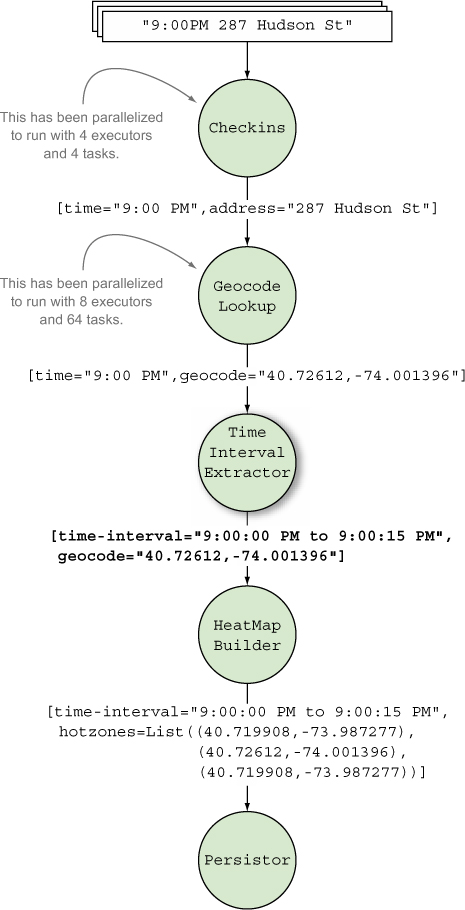
Figure 3.16 illustrates the parallelism changes that were just applied.

Figure 3.16. Parallelizing all the components in our topology

It looks like we’re done with scaling this topology...or are we? We’ve configured every component (that is, every spout and bolt) for parallelism within the topology. Each bolt or spout may be configured for parallelism, but that doesn’t necessarily mean it will run at scale. Let’s see why.

3.5.3. Adjusting the topology to address bottlenecks inherent within a data stream

We’ve parallelized every component within the topology, and this is in line with the technical definition of how every grouping (shuffle grouping, fields grouping, and global grouping) we use affects the flow of tuples within our topology. Unfortunately, it’s still not effectively parallel.

Although we were able to parallelize HeatMapBuilder with the changes from the previous section, what we forgot to consider is how the nature of our data stream affects parallelism. We’re grouping the tuples that flow through the stream into segments of 15 seconds, and that’s the source of our problem. For a given 15-second window, all tuples that fall into that window will go through one instance of the HeatMapBuilder bolt. It’s true that with the design changes we made HeatMapBuilder became technically parallelizable, but it’s effectively not parallel yet. The shape of the data stream that flows through your topology can hide problems with scaling that may be hard to spot. It’s wise to always question the impact of how data flows through your topology.

How can we parallelize this? We were right to group by time interval because that’s the basis for our heat map generation. What we need is an additional level of grouping under the time interval; we can refine our higher-level solution so that we’re delivering heat maps by time interval by city. When we add an additional level of grouping by city, we’ll have multiple data flows for a given time interval and they may flow through different instances of the HeatmapBuilder. In order to add this additional level of grouping, we first need to add city as a field in the output tuple of GeocodeLookup, as shown in the next listing.

Listing 3.14. Adding city as a field in the output tuple of GeocodeLookup.java

GeocodeLookup now includes city as a field in its output tuple. We’ll need to update TimeIntervalExtractor to read and emit this value, as shown in the following listing.

Listing 3.15. Pass city field along in TimeIntervalExtractor.java

public class TimeIntervalExtractor extends BaseBasicBolt {
  @Override
  public void declareOutputFields(OutputFieldsDeclarer declarer) {
    declarer.declare(new Fields("time-interval", "geocode", "city"));
  }

  @Override

  public void execute(Tuple tuple,
                      BasicOutputCollector outputCollector) {
    Long time = tuple.getLongByField("time");
    LatLng geocode = (LatLng) tuple.getValueByField("geocode");
    String city = tuple.getStringByField("city");

    Long timeInterval = time / (15 * 1000);

    outputCollector.emit(new Values(timeInterval, geocode, city));
  }
}

Finally, we need to update our HeatmapTopologyBuilder so the fields grouping between TimeIntervalExtractor and HeatMapBuilder is based on both the time-interval and city fields, as shown in the next listing.

Listing 3.16. Added second-level grouping to HeatmapTopologyBuilder.java

Now we have a topology that isn’t only technically parallelized but is also effectively running in parallel fashion. We’ve made a few changes here, so let’s take an updated look at our topology and the transformation of the tuples in figure 3.17.

Figure 3.17. Adding city to the tuple being emitted by GeocodeLookup and having TimeIntervalExtractor pass the city along in its emitted tuple

We’ve covered the basics of parallelizing a Storm topology. The approach we followed here is based on making educated guesses driven by our understanding of how each topology component works. There’s more work that can be done on parallelizing this topology, including additional parallelism primitives and approaches to achieving optimal tuning based on observed metrics. We’ll visit them at appropriate points throughout the book. In this chapter, we built up the understanding of parallelism needed to properly design a Storm topology. The ability to scale a topology depends heavily on the makeup of a topology’s underlying component breakdown and design.

3.6. Topology design paradigms

Let’s recap how we designed the heat map topology:

1. We examined our data stream, and determined that our input tuples are based on what we start with. Then we determined the resulting tuples we need to end up with in order to achieve our goal (the end tuples).
2. We created a series of operations (as bolts) that transform the input tuples into end tuples.
3. We carefully examined each operation to understand its behavior and scaled it by making educated guesses based on our understanding of its behavior (by adjusting its executors/tasks).
4. At points of contention where we could no longer scale, we rethought our design and refactored the topology into scalable components.

This is a good approach to topology design. It’s quite common for most people to fall into the trap of not having scalability in mind when creating their topologies. If we don’t do this early on and leave scalability concerns for later on, the amount of work you have to do to refactor or redesign your topology will increase by an order of magnitude.

Premature optimization is the root of all evil.

Donald Knuth

As engineers we’re fond of using this quote from Donald Knuth whenever we talk about performance considerations early on. This is indeed true in most cases, but let’s look at the complete quote to give us more context to what Dr. Knuth was trying to say (rather than the sound bite we engineers normally use to make our point):

You should forget about small efficiencies, say about 97% of the time; premature optimization is the root of all evil.

You’re not trying to achieve small efficiencies—you’re working with big data. Every efficiency enhancement you make counts. One minor performance block can be the difference in not achieving the performance SLA you need when working with large data sets. If you’re building a racecar, you need to keep performance in mind starting on day one. You can’t refactor your engine to improve it later if it wasn’t built for performance from the ground up. So steps 3 and 4 are critical pieces in designing a topology.

The only caveat here is a lack of knowledge about the problem domain. If your knowledge about the problem domain is limited, that might work against you if you try to scale it too early. When we say knowledge about the problem domain, what we’re referring to is both the nature of the data that’s flowing through your system as well as the inherent choke points within your operations. It’s always okay to defer scaling concerns until you have a good understanding of it. Similar to building an expert system, when you have a true understanding of the problem domain, you might have to scrap your initial solution and start over.

3.6.1. Design by breakdown into functional components

Let’s observe how we broke down the series of operations within our topology (figure 3.18).

Figure 3.18. The heat map topology design as a series of functional components

We decomposed the topology makeup into separate bolts by giving each bolt a specific responsibility. This is in line with the principle of single responsibility. We encapsulated a specific responsibility within each bolt and everything within each bolt is narrowly aligned with its responsibility and nothing else. In other words, each bolt represents a functional whole.

There’s a lot of value in this approach to design. Giving each bolt a single responsibility makes it easy to work with a given bolt in isolation. It also makes it easy to scale a single bolt without interference from the rest of the topology because parallelism is tuned at the bolt level. Whether it’s scaling or troubleshooting a problem, when you can zoom in and focus your attention on a single component, the productivity gains to be had from that will allow you to reap the benefits of the effort spent on designing your components in this manner.

3.6.2. Design by breakdown into components at points of repartition

There’s a slightly different approach to breaking down a problem into its constituent parts. It provides a marked improvement in terms of performance over the approach of breaking down into functional components discussed earlier. With this pattern, instead of decomposing the problem into its simplest possible functional components, we think in terms of separation points (or join points) between the different components. In other words, we think of the points of connection between the different bolts. In Storm, the different stream groupings are markers between different bolts (as the groupings define how the outgoing tuples from one bolt are distributed to the next).

At these points, the stream of tuples flowing through the topology gets repartitioned. During a stream repartition, the way tuples are distributed changes. That is in fact the functionality of a stream grouping. Figure 3.19 illustrates our design by points of repartition.

Figure 3.19. The HeatMap topology design as points of repartition

With this pattern of topology design, we strive to minimize the number of repartitions within a topology. Every time there’s a repartitioning, tuples will be sent from one bolt to another across the network. This is an expensive operation due to a number of reasons:

• The topology operates within a distributed cluster. When tuples are emitted, they may travel across the cluster and this may incur network overhead.
• With every emit, a tuple will need to be serialized and deserialized at the receiving point.
• The higher the number of partitions, the higher the number of resources needed. Each bolt will require a number of executors and tasks and a queue in front for all the incoming tuples.

Note

We’ll discuss the makeup of a Storm cluster and the internals that support a bolt in later chapters.

For our topology, what can we do to minimize the number of partitions? We’ll have to collapse a few bolts together. To do so, we must figure out what’s different about each functional component that makes it need its own bolt (and the resources that come with a bolt):

• Checkins (spout)—4 executors (reads a file)
• GeocodeLookup—8 executors, 64 tasks (hits an external service)
• TimeIntervalExtractor—4 executors (internal computation; transforms data)
• HeatMapBuilder—4 executors (internal computation; aggregates tuples)
• Persistor—1 executor, 4 tasks (writes to a data store)

And now for the analysis:

• GeocodeLookup and Persistor interact with an external entity and the time spent waiting on interactions with that external entity will dictate the way executors and tasks are allocated to these two bolts. It’s unlikely that we’ll be able to coerce the behavior of these bolts to fit within another. Maybe something else might be able to fit within the resources necessary for one of these two.
• HeatMapBuilder does the aggregation of geocoordinates by time interval and city. It’s somewhat unique compared to others because it buffers data in memory and you can’t proceed to the next step until the time interval has elapsed. It’s peculiar enough that collapsing it with another will require careful consideration.
• Checkins is a spout and normally you wouldn’t modify a spout to contain operations that involve computation. Also, because the spout is responsible for keeping track of the data that has been emitted, rarely would we perform any computation within one. But certain things related to adapting the initial tuples (such as parsing, extracting, and converting) do fit within the responsibilities of a spout.
• That leaves TimeIntervalExtractor. This is simple—all it does is transform a “time” entry into a “time interval.” We extracted it out of HeatMapBuilder because we needed to know the time interval prior to HeatMapBuilder so that we could group by the time interval. This allowed us to scale the HeatMapBuilder bolt. Work done by TimeIntervalExtractor can technically happen at any point before the HeatMapBuilder:
  • If we merge TimeIntervalExtractor with GeocodeLookup, it’ll need to fit within resources allocated to GeocodeLookup. Although they have different resource configurations, the simplicity of TimeIntervalExtractor will allow it to fit within resources allocated to GeocodeLookup. On a purely idealistic sense, they also fit—both operations are data transformations (going from time to time interval and address to geocoordinate). One of them is incredibly simple and the other requires the network overhead of using an external service.
  • Can we merge TimeIntervalExtractor with the Checkins spout? They have the exact same resource configurations. Also, transforming a “time” to a “time interval” is one of the few types of operations from a bolt that can make sense within a spout. The answer is a resounding yes. This begs the question of whether GeocodeLookup can also be merged with the Checkins spout. Although GeocodeLookup is also a data transformer, it’s a much more heavyweight computation because it depends on an external service, meaning it doesn’t fit within the type of actions that should happen in a spout.

Should we merge TimeIntervalExtractor with GeocodeLookup or the Checkins spout? From an efficiency perspective, either will do, and that’s the right answer. We would merge it with the spout because we have a preference for keeping external service interactions untangled with much simpler tasks like TimeIntervalExtractor. We’ll let you make the needed changes in your topology to make this happen.

You might wonder why in this example we chose not to merge HeatMapBuilder with Persistor. HeatMapBuilder emits the aggregated geocoordinates periodically (whenever it receives a tick tuple) and at the point of emitting, it can be modified to write the value to the data store instead (the responsibility of Persistor). Although this makes sense conceptually, it changes the observable behavior of the combined bolt. The combined HeatMapBuilder/Persistor behaves very differently on the two types of tuples it receives. The regular tuple from the stream will perform with low latency whereas the tick tuple for writing to the data store will have comparably higher latency. If we were to monitor and gather data about the performance of this combined bolt, it’d be difficult to isolate the observed metrics and make intelligent decisions on how to tune it further. This unbalanced nature of latency makes it very inelegant.

Designing a topology by considering the points of repartitioning of the stream and trying to minimize them will give you the most efficient use of resources with a topology makeup that has a higher likelihood of performing with low latency.

3.6.3. Simplest functional components vs. lowest number of repartitions

We’ve discussed two approaches to topology design. Which one is better? Having the lowest number of repartitions will provide the best performance as long as careful consideration is given to what kind of operations can be grouped into one bolt.

Usually it isn’t one or the other. As a Storm beginner, you should always start by designing the simplest functional components; doing so allows you to reason about different operations easily. Also, if you start with more complex components tasked with multiple responsibilities, it’s much harder to break down into simpler components if your design is wrong.

You can always start with the simplest functional components and then advance toward combining different operations together to reduce the number of partitions. It’s much harder to go the other way around. As you gain more experience with working with Storm and develop intuition for topology design, you’ll be able start with the lowest number of repartitions from the beginning.

3.7. Summary

In this chapter, you learned

• How to take a problem and break it down into constructs that fit within a Storm topology
• How to take a topology that runs in a serial fashion and introduce parallelism
• How to spot problems in your design and refine and refactor
• The importance of paying attention to the effects of the data stream on the limitations it imposes on the topology
• Two different approaches to topology design and the delicate balance between the two

These design guidelines serve as best practices for building Storm topologies. Later on in the book, you’ll see why these design decisions aid greatly in tuning Storm for optimal performance.