5.2.1 Optical fiber concepts

Optical fibers generally consist of a fused silica (SiO₂) core and cladding. During drawing of the optical fiber, dopants are added to the silica to provide an index of refraction distribution throughout the cross-section of the optical fiber,¹ with the core index normally higher than the cladding. Typical core diameters are 5–10 μm for single-mode optical fibers and greater than 50–200 μm for multi-mode optical fibers. The cladding diameter for almost all single-mode optical fibers is standardized at 125 μm to permit easy interconnection. Small diameter fibers (80 μm) have also been developed for sensing applications.² The small diameter makes the fiber sensor less invasive when the fiber is embedded in a host material system, and increases the sensitivity of the sensor to applied loads. It can also allow smaller bending radii.

The cross-section of a step-index optical fiber is shown in Fig. 5.2. The index of refraction distribution is only a function of the radius with

$\begin{array}{l}\mathit{n}\left(\mathit{r},\mathit{\theta }\right)={\mathit{n}}_1\mathit{r}\le \mathit{a}\\ \mathit{n}\left(\mathit{r},\mathit{\theta }\right)={\mathit{n}}_2\mathit{a}<\mathit{r}\le \mathit{b}\end{array}$ [5.1]

[5.1]

In order for propagation of guided lightwaves to occur, n₁ > n₂. The index of refraction difference between the core and cladding is typically less than 1%.³

Each component of the lightwave propagating along the fiber in the z direction has the form,

$\mathit{\psi }\left(\mathit{r},\mathit{\theta },\mathit{z},\mathit{t}\right)=\overline{\mathit{\psi }}\left(\mathit{r},\mathit{\theta }\right){\mathrm{e}}^{\mathit{t}\left(\mathit{\omega t}-\mathit{\beta z}\right)}$ [5.2]

[5.2]

where $\overline{\mathit{\psi }}\left(\mathit{r},\mathit{\theta }\right)$ is the energy distribution in the plane perpendicular to the propagation direction, ω is the angular frequency (ω = 2πc/λ where c is the speed of light in a vacuum and λ is the free-space wavelength of the light-wave), t is time, and β is the propagation constant of the mode (phase shift per unit length). Each propagating mode has an effective index of refraction, n_eff = βλ/(2π). n_eff corresponds to the index of refraction of an equivalent homogeneous material for which the wave would propagate with the same propagation constant β as through the step-index fiber. For guided modes, n₂ < n_ett < n₁. The effective index of refraction n_eff, or mode propagation constant β, will play a critical role in the response of many optical fiber sensors. Although the step-index fiber is the easiest for which to analyze mode propagation, most commercially available optical fibers have different index distributions as shown in Fig. 5.3.¹ While most optical fiber manufacturers do not provide detailed information on the index distributions, they do provide data such as the core radius, design operating wavelength, and n_eff at common wavelengths (see for example Reference 4). From this information, the user can calculate the response of the optical fiber sensor using the same principles as for the step-index fiber.

The number of guided modes that can propagate through the optical fiber at a particular wavelength depends upon the normalized frequency at that wavelength, V,

$\mathit{V}=\frac{2\mathit{\pi }}{\mathit{\lambda }}\mathit{a}\sqrt{{\mathit{n}}_1^2-{\mathit{n}}_2^2}$ [5.3]

[5.3]

The first mode, also called the fundamental mode, propagates at all values of V. All other modes have a cutoff value of V below which it cannot propagate. The cutoff value for the second mode is at V = 2.4048. Therefore, for V < 2.4048 the fiber is referred to as a single-mode fiber, and for V > 2.4048 the fiber is referred to as a multi-mode fiber. For several sensing technologies it is important to utilize fibers that are single-mode at the wavelength to be interrogated so that the mode of propagation and coupling are welldefined. Additionally, the fundamental mode is the least affected by bending losses, as the energy is concentrated in the center of the fiber. Multi-mode sensors do exist and are generally easier to practically couple to instrumentation as the fiber core is larger and the modes are more spread out throughout the fiber cross-section.^5–10

Finally, additional modes, called cladding modes, are possible due to the interface condition between the outer diameter of the fiber and the surrounding medium, typically polymer coating or air. The form of these modes depends upon the index of refraction of the surrounding medium, n₃, and is present in the case of n₃ < n₂. The cladding modes can be excited locally in long period grating (LPG) sensors and exploited for the measurement of cure monitoring, chemical, or environmental sensing.¹¹

A second important class of optical fibers applied for sensing is highbirefringence fibers, also referred to as polarization maintaining (PM) fibers.¹² PM fibers present an index profile that is not rotationally symmetric and therefore propagate two separate, linearly polarized fundamental modes (LP₀₁) at two separate propagation constants, β₁ and β₂. The modes are polarized about orthogonal axes, referred to as the fast and slow axes. As the polarization axes are orthogonal, the two modes do not interfere with one another as they propagate along the optical fiber. These orthogonal modes can be used to independently measure multiple parameters. In other cases, only one of the two polarizations propagates, while the other is suppressed.

Standard fused silica fibers are linear elastic until failure for the following material properties: the elastic modulus E = 72 GPa, Poisson’s ratio v = 0.20, and thermal expansion coefficient a = 5.5 × 10^− 7/°C.¹³ Typical elongation at failure is 2–5%. A second common material class used for optical fibers is polymers. Polymer optical fibers (POF) have considerably lower stiffness than silica fibers, with E = 2.4–3.0 GPa and v = 0.34.¹⁴ Their stress-strain response is also extremely sensitive to strain rate, temperature, humidity, and hysteresis effects. POF fibers can have elongations at failure of up to 100% or more.

The attenuation spectrum of a silica optical fiber can be seen in Fig. 5.4. Three primary transmission windows are therefore used in telecommunication applications: around (1) 850 nm, (2) 1300 nm, and (3) 1550 nm. The same three transmission windows are typically used for optical fiber sensors due to the relative low-cost, wide selection, and high quality of components including optical fibers, couplers, and laser sources available for telecommunications applications. POFs demonstrate considerably more attenuation at near-infrared wavelengths than fused silica fibers;¹⁴ therefore POF sensors most often operate in the visible wavelength ranges.

5.2.2 Sensing mechanisms

External sensing parameters are generally encoded into changes within lightwaves propagating through an optical fiber in one of four manners, summarized in Fig. 5.5. The intensity of the lightwave propagating through an optical fiber can be modified through microbending of the optical fiber, a change in coupling from the fundamental mode to other non-guided modes, fracture of the optical fiber, or a change in power coupled into the fiber or from one fiber to another. Measuring the intensity of the propagating lightwave is relatively simple; however, light sources themselves often fluctuate in intensity. Feedback control loops can be applied to reduce these fluctuations, or the illuminating lightwave divided to create a reference intensity, as shown in Fig. 5.6a. Under these conditions, intensitybased sensors can provide absolute measurements, meaning that they are insensitive to power interruptions between data collections. One drawback to intensity-based sensors, however, is that they cannot be multiplexed for sensor networks.

The application of strain or temperature to an optical fiber changes the optical path length traversed by the lightwave as it propagates a distance L through the fiber, n_eff L. As the phase of the lightwave cannot be measured directly, the lightwave is generally re-combined with a reference lightwave from the same laser source (so that the two are coherent). When the reference lightwave is not exposed to the parameter to be measured, the relative phase shift between the signais can be related to the applied strain or temperature. The phase modulation is extremely sensitive to strain and therefore can provide very accurate measurements;¹⁵ however, the measurement of phase shift is not absolute due to the signal periodicity and is therefore affected by power interruptions between data collections. Techniques to alleviate these problems, such as low-coherence interferometry, are discussed later in this chapter. The reference signal can be completely sheltered from external parameters, or used for compensation of unwanted measurands such as temperature, if both fibers are exposed to them.

External sensing parameters can also be converted into spectral information of the lightwave, for example using fiber Bragg gratings (FBG) or Fabry–Pérot interferometers. Such sensors typically act as filters, transmitting certain wavelengths and radiating or reflecting others. Changes in external parameters are therefore converted into a wavelength shift of the transmitted or reflected spectrum of the sensor. A typical signal is shown in the example of Fig. 5.5, for which the reflected wavelength is changing with time. The wavelength encoded signal must then be interpreted, which is commonly performed in using one of three methods: (1) by launching a broadband of light into the fiber and applying a spectrum analyzer to select the reflected wavelength; (2) by applying a tunable laser for which the output wavelength can be scanned while the reflected intensity is measured by a photodetector; or (3) by launching a broadband of light and using a wavelength dependent filter to identify the reflected wavelength (see Fig. 5.6b).

A final method to encode sensing information for transmission through an optical fiber is through the polarization state of the propagating lightwave.^15–17 For the example shown in Fig. 5.5, the power of a lightwave propagating through a PM fiber is transferred between the mode polarized about the fast axis and the mode polarized about the slow axis. The power in each mode can be determined by applying a polarizing filter or splitter to the output signal. As mentioned above, the two modes propagating through a PM fiber do not normally transfer power as they propagate, since they are orthogonally polarized. However, external stimuli such as pressure or twisting of the optical fiber will induce transfer between the two modes.

5.2.3 Sensor packaging

Traditional fiber optic cable design aims at the best possible protection of the fiber itself from any external influence. In particular, it is necessary to shield the optical fiber from external humidity, side pressures, crushing, and longitudinal strain applied to the cable. These designs have proven very effective in guaranteeing the longevity of optical fibers used for communication and can be used as sensing elements for monitoring temperatures in the − 20 °C to + 60 °C range e.g. in conjunction with Brillouin or Raman distributed sensing systems.

However, many of the measurement techniques described in Section 5.2.2 require that the sensing part of the optical fiber is exposed to the parameter to be measured. This creates a challenge for the sensor designer, to protect the sensor from damage resulting from manipulation and exposure to the environment while at the same time allowing a faithful transfer of the measurand from the object under monitoring to the optical fiber.^18,19

Special cable designs using non-standard coatings and buffers are required for sensing temperatures below − 20 °C or above + 60 °C, especially for Brillouin scattering systems, where it is important to guarantee that the optical fiber does not experience any strain that could be misinterpreted as a temperature change due to the cross-sensitivity between strain and temperature.

For strain and deformation sensors, the packaging must faithfully transfer the structural strain to the optical fiber, a goal contradicting all experience from telecommunication cable design where the exact opposite is required. This can be achieved by a continuous mechanical coupling between the sensor and the structure e.g., by continuously gluing the fiber to a steel beam, or by a local coupling at the ends of the sensing zone.²⁰

All sensor packaging designs share common reliability goals independently from the sensing technique and application domain used:

5.2.4 Cables, connectors, and splicing

The above considerations on sensor packaging also apply to the interconnection cables, connectors, and splices. In most cases it is however possible to borrow tools and techniques widely used in the telecommunication industry. Cables with different levels of protection are to be used depending on their location: indoor, outdoor, overhead, rodent-resistant, compatible with extreme temperatures, presence of radiation, or chemically aggressive environments.

Standard telecom connectors can be used in junction boxes, but more rugged versions for direct exposure to the elements also exist. Examples include outdoor and waterproof connectors, up to extreme cases such as deep-water remotely operated underwater vehicle (ROV)-matable connectors. Splicing is considered a more reliable way to permanently interconnect optical fibers, but requires tools and expertise that are not always compatible with field conditions. Therefore, an accurate analysis of the project will lead to the appropriate choice of a connector, a splice, or a very long cable.

5.3.1 Coherent interferometers

Butter and Hocker²¹ demonstrated the first in-fiber strain sensor. This ‘fiber optics strain gage’ was based on the measurement of the change in phase shift of a lightwave propagating through an optical fiber. The phase shift was due to applied axial strain through both the elongation of the optical fiber and the material property change of the silica with strain. The phase shift measurement replicated a conventional bulk optic coherent interferometer. Coherent, in-fiber interferometric sensors such as this present an extremely high sensitivity to external parameters. Additionally, as the optical fiber itself is used as the measurement device, such sensors are beneficial for simplicity and cost when compared to other optical fiber-based sensors.

Applying an axial tension to an optical fiber of length L, with a resulting axial strain ε, and a uniform temperature change, ΔT, along the entire optical fiber, we find the change in phase shift, Δφ, of a lightwave propagating through the fiber by:

$\mathrm{\Delta }\mathit{\phi }\mathit{=}\frac{2\mathit{\pi }}{\mathit{\lambda }}{\mathit{n}}_{\mathrm{eff}}\mathit{L}\left\{\mathit{\epsilon }-\frac{1}{2}\mathit{\epsilon }{\mathit{n}}_{\mathrm{eff}}^2\left[{\mathit{p}}_{12}-\mathit{v}\left({\mathit{p}}_{11}+{\mathit{p}}_{12}\right)\right]+\frac{1}{{\mathit{n}}_{\mathrm{eff}}}\frac{\mathit{d}{\mathit{n}}_{\mathrm{eff}}}{\mathit{dT}}\mathrm{\Delta }\mathit{T}+\frac{{\mathit{n}}_{\mathrm{eff}}^2}{2}\left({\mathit{p}}_{11}+2{\mathit{p}}_{12}\right)\mathit{\alpha }\mathrm{\Delta }\mathit{T}\right\}$ [5.4]

[5.4]

where λ is the wavelength of the lightwave.²² The phase shift is therefore linearly proportional to the applied strain and the applied temperature change. Typical material property values for fused silica are p₁₁ = 0.17, p₁₂ = 0.36, a = 0.5 × 10^− 6 °C^− 1, and dn_eff/dT= 1.2 × 10^− 5 °C^− 1.²²

The above equations consider a constant strain field applied along the gage length of the optical fiber. In general, the fiber can be mounted in any orientation on a surface, therefore these strain components can also vary along the length of the gage. We find the total phase shift by integrating the local phase shift along the optical fiber

$\mathit{\phi }={\displaystyle {\int }_0^{\mathit{L}}\left(\frac{\mathit{d\phi }}{\mathit{ds}}\right)}\mathit{ds}=\left(\frac{2\mathit{\pi }}{\mathit{\lambda }}\right){\displaystyle {\int }_0^{\mathit{L}}{\mathit{n}}_{\mathrm{eff}}}\left(1-{\mathit{p}}_{\mathit{e}}\right)\left(1+{\mathit{\epsilon }}_{\mathit{n}}\right)\mathit{ds}$ [5.5]

[5.5]

where ε_n is the strain component tangent to the fiber path at each location and s is the variable along the path length.²³ The transfer of shear stress and transverse stresses are negligible for surface mounted sensors, however, these components could be significant for sensors embedded in materials.^22,24

When using an optical fiber as strain sensor, it is not possible to measure the phase shift directly; therefore, we typically measure the interference between the sensor fiber and a second reference fiber that is not exposed to the environmental changes and therefore has a constant phase. Additionally, this second fiber can be exposed to only some of the loading, for example temperature, so as to provide compensation during the measurements. The interferometric measurement of phase shifts for in-fiber sensors parallels that for classical free-space interferometers. The two most commonly applied interferometric arrangements are the Mach-Zehnder and Michelson interferometers.²⁵ Figures 5.7 and 5.8 show each of these classical interferometers and their equivalent for in-fiber sensors. These are typical examples of long-base sensors.

Assuming that the light source has a high coherence length, and polarization effects are compensated between the two fibers, the average intensity of the interference pattern varies sinusoidally, as shown in Fig. 5.9. The cyclic form of the intensity measurement presents two challenges when the intensity is near one of the quadrature points i.e., where dI/dφ = 0. The first challenge is that the direction of fringe movement cannot be determined at the quadrature point (directional ambiguity), and the second is that the measurement sensitivity goes to zero at the same point (signal fading). A variety of signal processing techniques have been applied to remove these difficulties, generally categorized into passive and active demodulation.^26–28 One example of a passive homodyne demodulation is shown in Fig. 5.9. For this example, the sensor lightwave is divided into two channels, with one phase shifted by 90°, and the other interfered with the reference lightwave. When one signal is near a quadrature point, the other is at the point of maximum sensitivity, removing both the signal fading and directional ambiguity issues.

Furthermore, the measurement of phase shift is not an absolute measurement. Specifically, in order to know the current strain level, the system must be continually operated throughout the lifetime of the structure with a sufficient data acquisition frequency to catch every shift of more than half wavelength. This presents significant challenges for continuous monitoring of structures, since power interruptions lead to a loss of the zero point calibration. One solution to this problem is through low-coherence interferometry, which will be described in the following section. Another challenge is multiplexing interferometric based sensors. Kersey²⁹ reviews multiplexing strategies for interferometric optical fiber sensors, including time-division multiplexing (TDM) and frequency-division multiplexing examples.

5.3.2 Low-coherence interferometers

The light source used in an interferometer sensor is never pure and always contains a spectrum of wavelength distributed around the main wavelength. This causes the sinusoidal interference pattern to fade in intensity with an increasing path difference between the two arms. This fading is faster if the spectral distribution of the source is larger. The path difference for which the interference intensity falls to 1/e is called the coherence length of the source. This negative effect for traditional interferometers can be used advantageously to obtain absolute measurements, while maintaining the high resolution typical of interferometric sensors. If a light source with very low coherence length (i.e. with a large spectral width) is used, the interference pattern will fade very quickly with increasing path imbalance. It is, however, possible to restore the interference if the light is passed through a second interferometer that matches the path imbalance in the sensor. If the path imbalance of the second interferometer can be controlled precisely, it becomes possible to measure the unknown path imbalance in the sensor with the same accuracy, by finding the matching condition that maximizes the fringe intensity. Examples of low-coherence sensors include the surveillance d’ouvrages par senseurs à fibres optiques (SOFO) sensors and Fizeau readout units for Fabry–Pérot Sensors (see next paragraph).

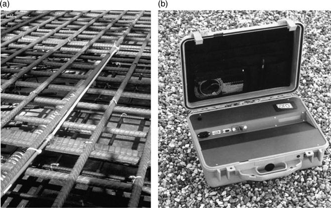
The SOFO interferometric sensors are long-base sensors, integrating the measurement over a long measurement base that can reach 10 m or more. The SOFO system^30,31 is a fiber optic displacement sensor with a resolution in the micrometer range and excellent long-term stability. The measurement set-up uses low-coherence interferometry to measure the length difference between two optical fibers installed on the structure to be monitored (Plate I in the color section between pages 294 and 295), by embedding in concrete or surface mounting (see Fig. 5.10a). The measurement fiber is pre-tensioned and mechanically coupled to the structure at two anchorage points in order to follow its deformations, while the reference fiber is free and acts as temperature reference. Both fibers are installed inside the same plastic pipe, and the gage length can be chosen between 200 mm and 10 m. The SOFO readout unit, shown in Fig. 5.10b, measures the length difference between the measurement fiber and the reference fiber, by compensating it with a matching length difference in its internal interferometer. The precision of the system is of ± 2 μm independently from the measurement basis and its accuracy of 0.2% of the measured deformation even over years of operation.

The SOFO system has been used in particular to monitor civil and geotechnical structures, including bridges,³² tunnels, piles,³³ anchored walls, dams, historical monuments,³⁴ and nuclear power plants, as well as laboratory models. The use of long-base SOFO sensors allows the gapless monitoring of the whole length of the structure, and provides average data that are not affected by local features or defects of the construction materials.

5.3.3 Fabry–Pérot interferometers

Fabry–Pérot interferometric sensors³⁵ are a typical example of point sensors and have a single measurement point at the end of the fiber optic connection cable. An extrinsic Fabry–Pérot interferometer (EFPI) consist of a capillary glass tube containing two partially mirrored optical fibers facing each other, but leaving an air cavity of a few microns between them, as shown in Fig. 5.11a. When light is coupled into one of the fibers, a back-reflected interference signal is obtained. This is due to the reflection of the incoming light on the two mirrors. This interference can be demodulated using coherent or low-coherence techniques to reconstruct changes in the fiber spacing. Since the two fibers are attached to the capillary tube near its two extremities (with a typical spacing of 10 mm), the gap change will correspond to the average strain variation between the two attachment points shown in Fig. 5.11a. Based on the same principle, it is possible to design pressure sensors (Fig. 5.11b) and displacement sensors (Fig. 5.11c).

Many sensors based on this principle are currently available as a one-to-one replacement of traditional sensors used in civil and geotechnical monitoring,³⁶ including piezometers, weldable and embedded strain gages, temperature sensors, pressure sensors, and displacement sensors. Examples are shown in Fig. 5.12.

Because they are immune to electromagnetic interference, such as that found in railway applications, or the static electricity and frequent thunderstorms that are found in dams at high altitudes, fiber optic instruments offer an important advantage over the traditional vibrating wire technology for those applications. They are more rugged in such a harsh environment and allow very long cable lengths without the need for any lightning protection.

5.3.4 Fiber Bragg gratings

Fiber Bragg grating (FBG) sensors have many advantages for strain sensing in structural health monitoring applications, including the ability to measure localized strain and temperature and the potential to multiplex hundreds of sensors with a single ingress/egress fiber. They are the most commonly used type of multiplexed sensor. FBG sensors have been applied for a variety of structural health monitoring applications including spacecraft,^37,38 bonded aircraft repairs,^39–41 cryogenic composite tanks,^42,43 highway and railway bridges,^44–47 offshore platforms,⁴⁸ and nuclear reactors.⁴⁹

The FBG, shown in Fig. 5.13, is a permanent, periodical perturbation in the index of refraction of the optical fiber core. Hill et al.⁵⁰ first fabricated permanent Bragg gratings in an optical fiber as a wavelength selective filter for telecommunication applications. When a broad spectrum of wavelengths is passed through the FBG, a narrow bandwidth of wavelengths is reflected, while all others are transmitted (see Fig. 5.13). The wavelength at maximum reflectivity is referred to as the Bragg wavelength, λ_B and is determined by the condition

${\mathit{\lambda }}_{\mathit{B}}=2{\mathit{n}}_{\mathrm{eff}}\mathrm{\Lambda }$ [5.6]

[5.6]

where Λ is the period of the index of refraction variation.

The reflectivity coefficient is defined as the ratio of the intensity of the input lightwave to that of the reflected lightwave, as a function of wavelength, and is given by:

$\mathit{r}=\frac{{sinh}^2\left(\mathit{L}\sqrt{{\mathit{\kappa }}^2-{\widehat{\mathit{\sigma }}}^2}\right)}{{cosh}^2\left(\mathit{L}\sqrt{{\mathit{\kappa }}^2-{\widehat{\mathit{\sigma }}}^2}\right)-\left({\widehat{\mathit{\sigma }}}^2/{\mathit{\kappa }}^2\right)}$ [5.7]

[5.7]

where κ and $\widehat{\mathit{\sigma }}$ a are the coupling coefficients defined as:

$\begin{array}{l}\mathit{\kappa }=\frac{\mathit{\pi }}{\mathit{\lambda }}\mathit{v}\overline{\mathit{\delta }{\mathit{n}}_{\mathrm{eff}}}\\ \stackrel{⌢}{\mathit{\sigma }}=\frac{2\mathit{\pi }}{\mathit{\lambda }}\left({\mathit{n}}_{\mathrm{eff}}+\overline{\mathit{\delta }{\mathit{n}}_{\mathrm{eff}}}\right)-\frac{\mathit{\pi }}{\mathrm{\Lambda }}\end{array}$ [5.8]

[5.8]

where L is the grating length, $\overline{\mathit{\delta }{\mathit{n}}_{\mathrm{eff}}}$ is the amplitude of the index of refraction modulation, and v is the modulation fringe visibility. For sensing applications, FBGs with a narrow bandwidth and high reflectivity produce the largest signal-to-noise ratio. Procedures such as apodization are often applied to the FBG sensor during fabrication to reduce the secondary peaks and narrow the bandwidth.⁵¹

As axial strain, ε, is applied to the FBG, the Bragg wavelength shifts to lower wavelengths (compression) or higher wavelengths (tension). The applied strain is thus encoded in the FBG Bragg wavelength shift. For the specific case of pure axial loading we find:

$\frac{\mathrm{\Delta }{\mathit{\lambda }}_{\mathit{B}}}{{\mathit{\lambda }}_{\mathit{B}}}=\left(1-{\mathit{p}}_{\mathit{e}}\right)\mathit{\epsilon }$ [5.9]

[5.9]

where p_e is the effective photo-elastic constant for axial strain. A typical value of p_e for silica optical fibers is 0.22–0.25.3⁵² Thus, the shift in Bragg wavelength is linearly related to the applied axial strain.

Similarly, FBG sensors are also sensitive to temperature through

$\frac{\mathrm{\Delta }{\mathit{\lambda }}_{\mathit{B}}}{{\mathit{\lambda }}_{\mathit{B}}}\left(\mathit{\alpha }+\mathit{\zeta }\right)\mathrm{\Delta }\mathit{T}$ [5.10]

[5.10]

where α is the thermal expansion coefficient and ζ is the thermo-optic coefficient of the optical fiber material. A typical value for fused silica is (α + ζ)= 6.67 × 10^− 6 °C^− 1.⁵² It is important to note that the thermal sensitivity of an FBG sensor is considerably higher than that of its electrical strain gage counterpart, increasing the need for thermal compensation for strain measurement applications.

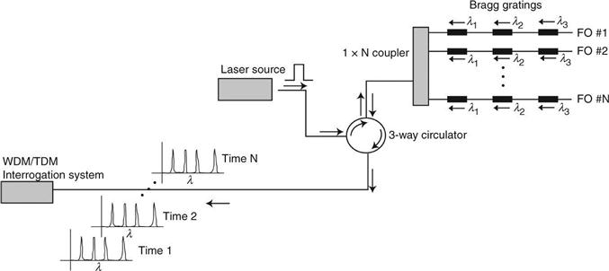
One of the strongest advantages of FBG sensors over other available strain or temperature sensors for structural health monitoring applications is the fact that they can be multiplexed into a large sensor network. For structural health monitoring applications, having only a single or limited ingress/egress points and lead cables is a notable advantage because it can significantly reduce the weight of the lead cables and disruptions to the structure itself.³⁷ Several approaches to multiplexing large FBG sensor networks have been applied in which the sensors are interrogated using wavelength-division and time-division multiplexing (WDM, TDM) and combinations thereof. For WDM applications, reducing the wavelength spacing between each FBG reduces the time required to scan the network, however also increases the cross-talk losses between FBGs. For TDM applications low reflectivity gratings (r_max ≅ 1%) should be used to allow for a large number of multiplexed sensors. By combining WDM with TDM, as shown in Fig. 5.14, one can reduce the power loss per FBG, as well as reducing the total wavelength range that must be scanned to interrogate the entire network.⁵² Several commercial interrogators are now available for networks of FBG sensors.^53–55 Interferometric methods have also been applied for high speed interrogation of FBG sensor networks.^56–58

FBG strain and temperature sensors can also distinguish between multiple strain components and/or temperature changes through the birefringence that occurs in the optical fiber due to applied transverse loads. Figure 5.15 shows an example of three independent loads applied to the optical fiber, along with the resulting three principal strain components at the center of the fiber core. The effect of the axial load (P₁) is to shift the reflected peak to higher or lower wavelengths; however, the effect of the transverse loads (P₂ and P₃) is to create peak-splitting due to the fast and slow axes that develop in the optical fiber. A typical example of peak-splitting behavior is also shown in Fig. 5.15. In general, FBGs written in PM optical fibers exhibit enhanced discrimination between multiple loading components.⁵⁹ The response of the FBG sensor to the multiple load components can either be predicted numerically^59–62 or experimentally calibrated.⁶³

Distortion of the grating spectrum due to strain gradients has also been observed in several applications of embedded FBG sensors.^64–73 An example of experimentally measured spectral distortion due to the highly nonuniform strain field near a notch tip is shown in Fig. 5.16.⁵⁴ This sensitivity of the sensor response to the form of the strain profile is unique to the optical FBG, since other strain gages (e.g., the classical electrical strain gage) average the applied strain over the gage length. This full-spectral information has been used to measure crack bridging distributions and damage states in laminates. Recently, Vella et al.⁷⁴ demonstrated a full-spectral interrogator that operates up to 100 kHz for dynamic measurements.

Finally, while FBGs reflect or transmit lightwaves at certain wavelengths based on coupling between counter-propagating core modes, long period grating (LPG) sensors are based on coupling between the forward propagating core mode and forward propagating cladding modes. The large period of the LPG (100 μm < Λ < 1 mm) results in cladding mode coupling at wavelengths in the near-IR range, appearing as multiple loss peaks in the transmission spectrum (see Fig. 5.17).⁷⁵ LPG sensors have primarily been applied to the measurement of environmental or chemical parameters due to their strong sensitivity to the index of refraction of the surrounding material system.

5.3.5 Brillouin and Raman scattering distributed sensors

Distributed fiber optic sensing offers the ability to measure temperatures and strains at thousands of points along a single fiber. This is particularly interesting for the monitoring of large structures such as dams, dikes, levees, tunnels, pipelines, and landslides, where it allows the detection and localization of movements and seepage zones with sensitivity and localization accuracy unattainable using conventional measurement techniques.

Unlike electrical sensors and localized FOSs, distributed sensors offer the unique characteristic of being able to measure physical parameters, in particular strain and temperature, along their whole length, allowing the measurements of thousands of points from a single readout unit. The most developed technologies of distributed FOSs are based on Raman⁷⁶ and Brillouin scattering.^77,78 Both systems make use of a nonlinear interaction between the light and the glass material of which the fiber is made. If an intense light at a known wavelength is shone into a fiber, a very small amount of it is scattered back from every location along the fiber itself. Besides the original wavelength (called the Rayleigh component), the scattered light contains components at wavelengths that are higher and lower than the original signal (called the Raman and Brillouin components). These shifted components contain information on the local properties of the fiber, in particular its strain and temperature. Figure 5.18 shows the main scattered wavelengths components for a standard optical fiber. If λ₀ is the wavelength of the original laser signal generated by the readout unit, the scattered components appear both at higher and lower wavelengths.

The two Raman peaks are located symmetrically to the original wavelength. Their position is fixed, but the intensity of the peak at lower wavelength is temperature dependent, while the intensity of the one at higher wavelength is unaffected by temperature changes. Measuring the intensity ratio between the two Raman peaks therefore yields the local temperature in the fiber section where the scattering occurred.

The two Brillouin peaks are also located symmetrically at the same distance from the original wavelength. Their position relative to λ₀ is however proportional to the local temperature and strain changes in the fiber section. Brillouin scattering is the result of the interaction between optical and ultrasound waves in optical fibers. The Brillouin wavelength shift is proportional to the acoustic velocity in the fiber that is related to its density. Since the density depends linearly on the strain and the temperature of the optical fiber, we can use the Brillouin shift to measure those parameters.

When light pulses are used to interrogate the fiber it becomes possible, using a technique similar to RADAR, to discriminate different points along the sensing fiber through the different time-of-flight of the scattered light. Combining the radar technique and the spectral analysis of the returned light, one can obtain the complete profile of strain or temperature along the fiber. Typically, it is possible to use a fiber with a length of up to 30 km and obtain strain and temperature readings every meter. In this case we would talk of a distributed sensing system with a range of 30 km and a spatial resolution of 1 m. Figure 5.19 schematically shows an example of distributed strain and temperature sensing.

Systems based on Raman scattering typically exhibit temperature accuracy of the order of ± 0.1 °C and a spatial resolution of 1–3 m over a measurement range up to 30 km. The best Brillouin scattering systems offer a temperature accuracy of ± 0.1 °C, a strain accuracy of ± 20 microstrain, and a measurement range of 50 km, with a spatial resolution of 1–3 m.⁷⁹ The readout units are portable and can be used for field applications.

Since the Brillouin frequency shift depends on both the local strain and temperature of the fiber, the sensor set-up will determine the actual response of the sensor. For measuring temperatures it is necessary to use a cable designed to shield the optical fibers from an elongation of the cable. The fiber will therefore remain in its unstrained state and the frequency shifts can be unambiguously assigned to temperature variations. Measuring distributed strains also requires a specially designed sensor. A mechanical coupling between the sensor and the host structure along the whole length of the fiber has to be guaranteed. To resolve the cross-sensitivity to temperature variations, it is also necessary to install a reference fiber along the strain sensor. Special cables, containing both free and coupled fibers, allow a simultaneous reading of strain and temperature. Figure 5.20 shows examples of temperature, strain, and combined cables.²⁰

Sensing systems based on Brillouin and Raman scattering are used to detect and localize seepage in dams and dikes, allowing the monitoring of hundreds of kilometers along a structure with a single instrument and the localization of the water path with an accuracy of 1 or 2 m. Distributed strain sensors are also used to detect landslide movements and to detect the onset of cracks in concrete dams and steel bridges.⁸⁰

Early applications of this technology have demonstrated that the design and production of sensing cables, incorporating and protecting the optical fibers used for the measurement, as well as their optimal locating and installation in the structure under scrutiny, are critical elements for the success of any distributed sensing instrumentation project.

5.4.1 Multicore fiber sensors

The recent fabrication of multicore optical fibers has led to new sensing capabilities for strain and temperature measurements. An example of a multicore optical fiber is shown in Fig. 5.21. The multiple cores are introduced with spacing sufficient such that there is minimal overlap between modes propagating through each core. These independently propagating modes permit the presence of multiple sensors in the same fiber cross-section. Coupling to the different cores is typically achieved by graded index lenses or fan-outs.⁸¹ The most common application of these multicore fiber sensors has been the measurement of curvature of different axes in the fiber cross-section by interfering the different propagating lightwaves or writing FBGs in the different cores.^82–84 As the cores are located at different locations relative to the neutral bending axes (see Fig. 5.21), the local curvature can be measured at high accuracies with inherent axial strain and temperature compensation. For example, Blanchard et al.⁸³ achieved a bend angle resolution of 100 μrad using a three-core optical fiber. By separating the multiple cores by polarization axes, the axial strain and temperature can also be measured independently.^85,86

Multiplexing FBG sensors along the fiber (in each of the different cores) have also been applied for high resolution shape sensing by integrating the local curvatures (about multiple axes) along the optical fiber length.^82,87,88 Flockhart et al.⁸⁹ and Cranch et al.⁹⁰ wrote sets of FBG pairs in each core to act as a low-finesse Fabry–Pérot interferometer to enhance the static and dynamic resolution of the distributed shape measurements.

5.4.2 Microstructured optical fiber sensors

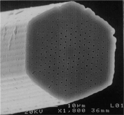
The recent invention of microstructured optical fibers has created great potential for both optical fiber communication systems and optical fiber sensors. Such fibers have a complex cross-sectional geometry including both silica and air holes. Confinement of the propagating lightwaves is generated either by an effective index contrast similar to that of conventional optical fibers in which the air holes significantly reduce the cladding index of refraction (‘holey’ fibers) or through a photonic bandgap effect (photonic crystal fibers).⁹¹ One example of a microstructure fiber is shown in Fig. 5.22. In either case, the complex geometry of these microstructured fibers provides both new sensing possibilities and enhanced response characteristics for sensors applied to these fibers.

For sensing applications the main potential benefits of these fibers are the following: (1) the reduced amount of silica through which the fundamental mode propagates means that the temperature sensitivity of the sensors can be reduced to near zero;⁹² (2) the fibers can act in single-mode over a wide range of wavelengths, permitting multiplexing of sensors at significantly different wavelengths;⁹³ (3) for chemical sensing applications, the gas to be sensed can be inserted into the air holes, permitting a long interaction surface between the propagating mode and the gas;⁹⁴ and (4) PM fibers can be fabricated through the arrangement of the air holes, without the need for induced thermal residual stresses, making the birefringence more stable to temperature variations.⁹⁵

Nasilowski et al.⁹⁵ and Bock et al.⁹⁶ applied microstructured holey fibers for the measurement of temperature and pressure. Several researchers have also written long period FBGs into microstructured fibers through CO₂ laser or electric arc etching.^97–99 These gratings demonstrate an excellent strain sensitivity, with little or no temperature sensitivity.^97,99 Finally, researchers have also succeeded in writing FBGs into photonic crystal optical fibers for use as discrete strain sensors.¹⁰⁰

5.4.3 Polymer optical fiber sensors

While the previous discussion has been limited to silica optical fibers, many of the same sensing techniques have been applied to polymer optical fibers (POFs) as well. POFs have additional advantages for sensing, such as their high elastic strain limit, high fracture toughness, high flexibility in bending, higher sensitivity to strain than silica, and negative thermo-optic coefficient.^101–104 Additionally, many polymeric materials have a high biocompatibility. More details on the properties of POFs can be found in References 14 and 105.

On the other hand, a significant challenge to applying POFs as sensors is the difficulties in fabrication of these fibers. Due to the fabrication difficulties, most POF sensors are based on multi-mode POFs.¹⁴ Multimode POFs are less expensive and easier to couple than silica singlemode optical fibers; however, they are also larger in diameter. POFs also demonstrate viscoelastic behavior and are extremely sensitive to humidity.^{102,104,106,107} Typical stress-strain curves for a POF at different applied strain rates are shown in Fig. 5.23. Additionally, many POF sensors operate at lower wavelengths than comparable silica fiber sensors, due to the high attenuation of polymers in the near-infrared range. Multi-mode POF sensors have been demonstrated based on many of the same measurement principles as silica optical fiber sensors, including intensity losses, back scattering, and time-of-flight.¹⁰⁸

Recently, both single-mode solid POFs and single-mode microstructured POFs have been developed that present new capabilities for POF sensors.^109,110 The emergence of these optical fibers has created the potential for high precision, large deformation optical fiber sensors for a variety of applications. Kiesel et al.¹¹¹ recently demonstrated coherent interferometry in a single-mode POF in-fiber Mach-Zehnder interferometer up to 15.8% elongation of the POF (see Plate II in the color section between pages 294 and 295). After calibration of both the mechanical and optomechanical parameters of the single-mode POF,^102,103 the authors applied the sensor for strain measurements on tensile coupons.¹¹² Additionally strategies to couple the single-mode POF sensor to single-mode silica optical fibers to remove the attenuation limits were developed.¹¹³ Peng et al.¹¹⁴ first demonstrated the writing of FBGs into single-mode POFs for localized strain sensing over large strain ranges. The POF FBG sensors demonstrate a 22% increase in strain sensitivity as compared to silica Bragg gratings¹¹⁵ and have been tuned over a 18 nm wavelength shift by applying a temperature change of 50 °C.¹¹⁶ Finally, van Eijkelenborg et al.¹¹⁷ fabricated microstructured POFs to overcome the high intrinsic attenuation properties of common POFs. These microstructured POFs have since been applied as sensors through inscribed LPGs and FBGs.^118–120

5.4.4 Rayleigh scattering distributed sensors

A more recent development in distributed fiber optic sensing is the use of Rayleigh backscattering for the interrogation of strain and temperature along an optical fiber. As for the previous distributed sensors, a standard optical fiber can be applied as the sensor, providing distributed measurements over large distances, without expensive individual sensors. Gifford et al.^121,122 applied swept-wavelength interferometry (SWI) to measure the backscattered signal in silica and POFs. This interrogation method is fundamentally different from optical time-domain reflectometry measurements, since SWI measures phase shifts rather than amplitudes in the backscattered signal. While the spectrum of the backscattered signal is random, it is deterministic. Local changes in temperature or strain create a wavelength shift in the response, similar to the effect measured by FBG sensors. Interrogating the backscatter spectrum with SWI can provide a high spatial resolution (up to 10 s of microns) with strain resolution up to 1 με and temperature resolution up to 0.1 °C.¹²¹ A similar set-up can also be used to produce a distributed acoustic sensor that can be used for intrusion detection and localization.