
Electromagnetic sensors for assessing and monitoring civil infrastructures
M.L. Wang, Northeastern University, USA
G. Wang, Chicago Bridge and Iron, USA
Abstract:
Electromagnetic sensors are non-destructive evaluation technologies and they are widely used in health monitoring and damage detection for infrastructures. In this chapter several existing technologies with various functional theories are briefly reviewed. The application of elastomagnetic (EM) (or magnetoelastic) stress sensor technology in stress monitoring for steel cables is described. The roles of microstructure and temperature in magnetization and magnetoelasticity are discussed. The design and configuration of an EM sensor are illustrated. In addition, the design of an appropriate energizing circuit to counteract eddy currents is introduced. Field application examples with EM sensors used in existing and new constructions are provided. A removable stress measurement design is also presented as a promising monitoring tool for steel structural components.
Key words
steel tendon stress monitoring; elasto-magnetic stress sensor; cable force monitoring; cable-stayed bridge; prestressed force monitoring; structural health monitoring; electromagnetic theory; non-destructive evaluation (NDE)
9.1 Introduction to magnetics and magnetic materials
Magnetic materials were initially utilized in compasses, as recorded in Chinese literature in the first century bc. In human civilization history, magnetic materials have contributed tremendously to navigation and geographic exploration. However, modern magnetic theory was established several centuries ago by the scintillating work of Gilbert, Ampere, Oersted, and others.
In this chapter, the magnetic properties of ferromagnetic materials are the main concern. In order to understand ferromagnetism, we first review the materials’ classification in accordance with their magnetic properties. The distinction between the materials in terms of magnetism lies in the interaction of the micromagnetic moment of the electron orbital motion and electron spinning, and the rearrangement of the moments caused by the applied magnetic field.
One can categorize inorganic materials into five groups: diamagnetic materials, paramagnetic materials, antiferromagnetic materials, ferromagnetic materials, and ferrimagnetic materials.1 In diamagnetic materials, such as copper, silver, gold, and beryllium, the magnetic moments introduced from electron spins and orbital motions counteract each other, which leads to a negligible magnetization even when exposed to an external field. While for paramagnetic materials such as aluminum, platinum, and manganese, the overall magnetization effect is an increase in the magnetization but weak within the materials. In super-paramagnetic materials, fine ferromagnetic particles are distributed in the non-ferromagnetic matrix; as a result, no magnetic memory remains due to thermal fluctuation.
In antiferromagnetic materials such as chromium, below the Neel temperature of 37 °C, under the applied magnetic field the neighboring atomic moments are antiparallel to each other, which leads to a zero net magnetization; therefore, such kind of materials are insensitive to a magnetic field. If the antiparallel moments sum up to a non-zero net magnetic moment, the material is called ferrimagnetic material, like Fe3O4, and can be considered as imperfectly antiferromagnetic.
Ferromagnetism occurs spontaneously in elements such as iron, nickel, and cobalt. In these elements, the magnetic moments are aligned in the same direction and are parallel to each other to produce strong magnets. The ferromagnetic materials can be either crystalline or amorphous, in which the atomic moments are aligned so as to achieve an intense magnetization higher than the applied field. At room temperature, the only ferromagnetic metals are iron, nickel, cobalt, and some alloys.
Experimental and theoretical analysis indicates that the basic functional unit in the ferromagnetic material is magnetic domain, which is a collection of atomic moments aligned in a parallel manner to minimize the exchange energy. The net magnetic moment within a domain is the summation of the atomic moments. The neighboring domains are separated by domain walls with a thickness of 10− 8 ~ 10− 6 m. The competition of the wall energy, crystal anisotropic energy, exchange energy, and magnetostatic energy determines the domain sizes, which however vary over a wide range.
Ferrimagnetic materials resemble ferromagnetic materials in such aspects as the structure of the magnetic domains and the phenomenon of hysteresis. In the ferrimagnetic materials, the magnetic moments within the neighboring sub-lattices compete with each other, and the net magnetization may demonstrate an unusual dependence on temperature, while the magnetization in ferromagnetic materials arises from the parallel alignment of the identical magnetic moments in one lattice. Otherwise, the net magnetization within all domains in ferromagnetic or ferrimagnetic specimen is zero, as indicated in Fig. 9.1.

If a ferromagnetic specimen is exposed to a magnetic field strong enough to magnetically saturate it, the magnetic domains will rotate until all are aligned unanimously, as shown in Fig. 9.2.

In ferromagnetic materials, the magnetizing process typically demonstrates the phenomenon of hysteresis, as shown in Fig. 9.3. There are three types of magnetic hysteresis curves. The first one is the major hysteresis curve, which depicts the variation in magnetic induction in the sample magnetized by the applied alternating field with a magnitude no lower than the technical magnetic saturation. Technical magnetic saturation means that the higher level of magnetization does not change the shape of the hysteresis. Magnetic parameters, such as remanence, coercivity, and saturated magnetization can be measured from major hysteresis curve. Owing to its high repeatability and straightforward measurability, major hysteresis is widely applied in physics and engineering.

The second type is the anhysteresis curve, which is plotted by applying a constant field superimposed with an oscillating field with descending magnitude escalating from positive saturation to zero. Each point on such curve is history-independent, and thus mainly dependent on material properties. Because of that, anhysteresis is valuable in material characterization. However, it takes a long time to complete the anhysteresis measurement, and the heat produced from the oscillating field can easily lead to a temperature rise.
The third type is the minor hysteresis curve, which is different from major hysteresis in that the magnitude of the alternating field is below technical saturation. The magnetic parameters can be defined in a similar way to major hysteresis, such as pseudo coercivity, pseudo remanence, pseudo hysteresis loss, and pseudo susceptibility, etc. Some parameters were reported to be more sensitive to a field than those derived from the major hysteresis loops.2 Confined in the major loop, the positions of the congruent minor loops depend on magnetization history; therefore, the minor loops are usually measured when the specimens are completely demagnetized.
The magnetic properties of the materials depend heavily on temperature. The ferromagnetic and ferrimagnetic materials will turn to be paramagnetic or antiferromagnetic (for some rare earth elements) when the temperature is raised above a threshold value such as Curie’s point. Antiferromagnetic materials will be paramagnetic above Neel’s point.
As materials technology evolves, specific magnetic phenomena and innovative magnetic materials are continually being brought forward. Various magnetic effects have already been industrialized, such as giant magnetore-sistance (GMR) – the magnetization dependence of the electrical conductivity, magnetocaloric effect – the magnetization dependence of the entropy, magnetorheological effect – the rheological properties of the magnetic powders suspended in viscous fluids, and magnetoelasticity. The magnetorheological effect has been used in magnetic dampers in infrastructures.3 Due to the proliferation in nano-technology, nano-magnetic materials have been intensively researched for their diverse applications in ferrofluids, drug delivery, radioactive tracer, and power conversion and conditioning.4 Magnetic shape memory, or ferromagnetic shape memory alloy, has also been studied.5
9.2 Introduction to magnetoelasticity
For most ferromagnetic materials, the magnetic performances are correlated with mechanical stress,6−12 which can be described in terms such as magnetoelasticity and magnetostriction. With a theoretical basis in magnetoelasticity, elastomagnetic (EM) stress sensors have been used successfully in health monitoring for infrastructures.13−16 Magnetoelasticity in ferromagnetic material is rooted in magnetic stress anisotropy. Several intrinsic and extrinsic factors lead to magnetic anisotropy, including crystal anisotropy, shape anisotropy, and anisotropy introduced by specific heat and mechanical treatment. Crystal anisotropy means that easy axis and plane magnetization requires relatively less amount of work; therefore, it is also called magnetocrystalline anisotropy. In non-cubic crystals, the magnetostatic interaction of atomic pairs and certain geometric arrangement of atoms generate crystal anisotropy.6 The shape anisotropy is indeed an extrinsic property induced by the direction-dependent demagnetization. Besides, magnetic annealing, stress annealing, plastic deformation, and magnetic irradiation can also induce magnetic anisotropy, owing to the preferential diffusion or sliding of the interstitial and substitutional atoms in favor of energetic equilibrium.7
As to magnetic stress anisotropy, applied or residual mechanical stress affects magnetization in respect to three mechanisms – first, magnetoelastic energy rotates magnetic moments and rearranges domain structures; second, stress introduces pressure on domain walls; third, stress changes the opposite terms that are balanced for domain wall equilibrium.9
The summation of magnetoelastic, magnetostatic, and magnetic anisotropic energy can be expressed as:10
[9.1]
H is the applied magnetic field, λs is magnetostrictive coefficient, B is flux density, and σ is tension. Ms is saturated magnetization, where θσ is the angle between stress axis and local magnetization, θH is the angle between applied field and local magnetization, and θD is the angle between shape anisotropy and local magnetization.
Thermodynamically, under equilibrium of magnetostatic and magnetoelastic energy, magnetoelasticity can be expressed as:11
[9.2]
where l is the length of the sample, H is the applied magnetic field, B is flux density, and σ is tension.
Equation [9.2] can be rewritten as
[9.3]
where μr is relative permeability.
In order to present the effect of stress on magnetization, the following equation can be drawn:11
[9.4]
where K is magnetic anisotropy constant, and N is a constant with a value of three for steel.11 It can be seen that if λS dσ > 0, the magnetization increases with tension.
Alternatively, the magnetization M under applied tension σa and magnetic field H is expressed in Reference 8
[9.5]
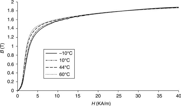
Equations [9.1] through [9.4] are derived with the assumption that no magnetic anisotropy is present except stress anisotropy. However, in a real situation, crystal anisotropy is usually more dominant than stress anisotropy in steels.7 In steels magnetoelastic behaviors can be demonstrated in the measurement of magnetizing curves under different stress levels, as indicated in Fig. 9.4.

The magnetization behavior of the steel is largely determined by its metallographic characteristics, which have been exploited extensively by researchers. Byeon and Kwan have studied the magnetic properties of specific metallurgical phases in plain steels, and revealed that the coercivity and remanence decrease in the order of martensite, pearlite, and ferrite phase.12 The aforementioned parameters are also susceptible to microscopic variation in the same type of microstructure. For example, the coercivity and remanence drop as the interlamellar spacing in pearlite increases, due to the reduction in both residual stress and pinning energy against domain wall movements.12−18 Besides, magnetization is sensitive to the formation of magnetic phases from nonmagnetic matrix.7 Therefore, coercivity, remanence, and hysteresis loss can be employed to monitor the material degradation and microstructure evolvement,19 such as fatigue and creep. Chemicals also play an important role in magnetic behavior of steels. The alloy elements affect magnetization significantly, since they raise the inner stress level owing to crystal distortion and interphase particles, which nail down the domain walls.
Magnetization and magnetoelasticity have been used in non-destructive evaluation (NDE) for steel or metallic components or structures. In magnetoelastic stress sensor, relative permeability is used to monitor the tensile stress.13−15 In the ensuing sections, key factors regarding the application of this technology will be addressed.
9.3 Magnetic sensory technologies
In pre-stressed concrete structures and cable-stayed bridges, knowing the static stress in critical steel structures is extremely important for safety and reliability of structures. Catering to this requirement, magnetoelastic stress sensory technology has been developed. Prior to proceeding in this topic, some representative developments and practices in NDE using magnetic technologies are reviewed.
As of today, a series of monitoring technologies have been conceptualized and developed in order to inspect or characterize steel or metallic structures or components, and their health and degrading conditions. Below are some typical magnetic NDE approaches for metallic materials and structures:
1. Microstructural characterizing using magnetic method: Several magnetic parameters including magnetic coercivity and permeability are exterior characteristics of ferromagnetic materials. The microstructure characteristics, such as the content of non-ferromagnetic phases, the relative amounts of different phases, and the characteristics of precipitations, affect one or several readings of the magnetic parameters. For example, creep-induced microstructure degradation was tentatively characterized via magnetic measurement.19,20 The magnetic phase constitution gage is a promising tool in monitoring phase transformation. A type of supercon-ducting quantum interference device (SQUID) unit was developed in order to evaluate the transformation of d-ferrite to nonmagnetic phases during fatigue in welded steels.21 The precondition in favor of the feasibility of this technology is that the adverse influence of microstructure or geometric anisotropy must be calibrated.
2. Geometric/structural discontinuity (for example, cracks) inspection using magnetic method: Conventionally, heat treatment and welding cracks are to be detected by the method of magnetic powder inspection. In this method, the discontinuity of magnetic loops can identify structural anomalies. In a magnetic loop composed of magnetic flux emitter and steel component to be monitored, the magnetic flux constitutes a closed loop. If a structural discontinuity exists on the component to be monitored, the magnetic flux will be detected, from which the structural deformation, cracks, and other types of anomalies can be mapped. For example, the portable U-shape sensory system16 shown in Fig. 9.5 can be used for crack inspection in steel ropes.
3. Anomaly inspection through dynamic magnetic signal (eddy current and Barkhansen noise, and so on): Geometric discontinuity and materials/microstructure variation can be monitored through eddy current and the induced magnetic field, and the jump of magnetic domains. This approach has been used in detecting metallurgical failure in components such as fractures caused by stress corrosion and hydrogen embitterment; the proactive prognostic inspection of the latter can prevent catastrophic component failures.
4. Corrosion monitoring using magnetic method: Based on the theory of magneto-hydrodynamics, a magnetic field affects the mass transport rates and electro-transferring process in galvanic reactions;22 on the other hand, the latter also generates certain kinds of magnetic field. It was found that with catholic protection current, a corrosion-related magnetic (CMR) field is introduced,23 as shown in Fig. 9.6. Most metals and alloys tend to be corroded in the environment into which they were exposed, for instance the corrosion of pre-stressed tendons with exposure to liquid solution or condensates. Galvanic reaction can be used to describe the progress of this kind of corrosion.
Through anodic reaction metallic atom, M, gives up one or more electrons to become a cation:
[9.6]
The cathodic reaction can be either
[9.7]
or
[9.8]
In galvanic corrosion, transportation of anions and electrons is involved, therefore an electric current exist in reaction.
According to Maxwell Equations:23
[9.9]
where ![]() is vector potential and
is vector potential and ![]() is vector of current density.
is vector of current density.
The magnetic field thus introduced can be expressed as:
[9.10]
Through the inspection of this field, the galvanic corrosion can be estimated.
A magnetic sensor for corrosion monitoring based on loss and degradation of magnetic characteristics of corroded article is also a promising approach to evaluate the conditions of corrosion. For example, Yashiro et al. developed a method to detect the environmental deterioration of the structure by measuring the decrease in residual magnetization on probes embedded in mortar.24 Analogous to crack inspection using magnetic methods, metallic loss or other irregularities caused by corrosion can be inspected via magnetic leakage methods.25 More work needs to be carried out to industrialize corrosion monitoring technology through measuring and mapping of magnetic fields.
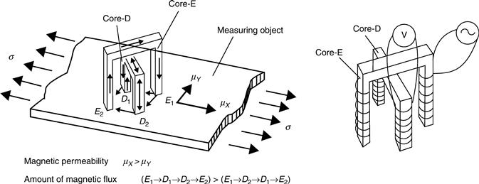
5. Mapping and characterizing residual stress in steel structures using magnetic method: For some steel structures like railway rails, knowing the amplitude, direction, and sign of residual stress is useful for proper maintenance and failure prevention.26 Due to stress magnetic anisotropy, the existence of local residual stress in steel changes its magnetic properties of the related steel section. The magnetic measurement equipment is able to deliver the required measurement resolution and can specify and map the distribution of the residual stress. The magnetic anisotropy and permeability system (MAPS) indicated in Reference 26 is a promising tool for this purpose. Depending on the interaction of residual stress and magnetization in multiple mini-scaled regions, the residual stress on a rail can be mapped, as seen in Fig. 9.7.
A magnetic anisotropy sensory approach for similar purposes was reported in Reference 27, with the configuration shown in Fig. 9.8.
6. Magnetostrictive sensors: In magnetostrictive materials, the magnetic properties vary as a function of applied stress; this phenomenon is called the inverse magnetostrictive effect, or the magnetomechanical effect and the same operating principle was used for the accelerometer.28 Made primarily of amorphous ferromagnetic ribbons or wires, magnetostrictive elastic sen-sors have been used in measuring a wide range of environmental parameters, including pressure, humidity, temperature, liquid viscosity and density, thin-film elasticity, chemicals such as carbon dioxide and ammonia, and pH value. One example is the application of the resonant frequency in a magnetostrictive material. Excited by a wave induced by AC magnetic field, the resonant frequency of the magnetostrictive wire or strip depends on density, Young’s modulus, and Poisson ratio of the sensor. The characteristic resonant frequency is also dependent upon the magnitude of the DC biasing field, the ambient medium, and the sensor surface condition including surface roughness and wetting, and also the surface stress. Therefore, physical or environmental variation in the magnetostrictive agent will change the resonant frequency.29,30 Innovative materials with large magnetostrictive coefficients are key to yielding high sensitivity in these kinds of magnetostrictive sensors; gallium alloy is a good example.5
7. Application of magnetoelasticity in tensile stress monitoring: This topic is the main subject and is covered in the following sections in detail. The method is used to monitor new steel cables during construction, as well as existing cables in service. Emphasis is on continuing monitoring for a period of time to effectively assess the overall structural health as well as to determine tension forces in cables, an important parameter for maintenance of cabling systems.


9.4 Role of microstructure in magnetization and magnetoelasticity
In magnetoelastic stress sensors, magnetic relative permeability is used to reflect stress level in steel structures. Zero-stress saturated permeability (permeability at technical magnetic saturation with no stress applied on the steel rod) defines the stress-free status of the steel to be monitored.12−16
Magnetic permeability implies the realigning tendency of magnetic domains in response to an exterior magnetic field. Metallurgical characteristics strongly influence magnetic permeability. The hardness represents the mechanical stiffness of the material and depends on multiple metallurgical characteristics, including composition, phase constitutes and morphology, residual stress, and grain size, etc. Those factors also play roles in pinning effects against magnetic domain reorientation. The correlation of hardness with permeability is demonstrated in Fig. 9.9 and Table 9.1. It can be seen that the harder the ferromagnetic steel, the lower the initiative permeability. There are several causes for this observation – (I) the amount of the ferrite phase decreases as carbon content increases, and ferrite is magnetically the softest microstructure in steel; (II) the carbides or other precipitates function as pinning particles against domain reorientation; (III) cold work, lattice defect, and even heat treatment and welding can introduce intrinsic (residual) stress, which decreases the initiative permeability due to the pinning effect; (IV) besides, specific intrinsic stresses lead to a certain level of magnetic anisotropy – one example is that in cold extruded steel rod, the longitudinal residual compressive stress introduces a magnetic anisotropy and a fictitious field;21 as another example, in material with non-zero magnetostriction, magnetization can be introduced on the cutting edge of the sample,31 owing to the influence of residual stress on magnetic moments and domains. This phenomenon can be used in NDE for geometric non-continuity in steels. Similar effects can be observed in welding.32

Table 9.1
Hardness of various carbon/alloy steels tested in Fig. 9.4
| Steel | Microhardness (HV at 500 g) |
| 1018 cold drawn | 217 |
| 8620 annealed | 230 |
| 4140 annealed | 240 |
| 1045 cold drawn | 331 |
| Piano steel wire | 467 |
As indicated in Figs 9.10 and 9.11, the magnetic hysteresis and saturated permeability in steels depend on their relative heat treatments. The saturated permeability increases as hardness drops, with the exception of the as-received cold-drawn steel rod because of magnetic anisotropy caused by residual stress generated by cold drawing process.


For the EM stress sensor, relative incremental permeability under technical magnetic saturation is the parameter used for stress monitoring, as shown in Figs 9.12 and 9.13.


With load well below elastic limit, magnetic permeability varies monotonically with tensile stress. When the tension increases beyond yielding point, the permeability first reaches its summit and then drops, as indicated in Fig. 9.14, due to the collaborative effects of magnetoelasticity and metallurgical dislocation multiplication. Although the tensile stress tends to raise the relative permeability, the latter declines once the influence of multiplying dislocations takes the control.

9.5 Magnetoelastic stress sensors for tension monitoring of steel cables
As shown in Fig. 9.12, magnetic permeability demonstrates strong sensitivity to load at all magnetization levels, especially at low magnetization level; however, due to the drawback of minor hysteresis with magnetic offset superseded, permeability under low magnetization level is not recom-mended for stress monitoring. In EM tensile stress sensors presently being actively commercialized, the relative permeability is calculated from the integration of the output of the secondary coil. The sensor configuration is indicated in Fig. 9.15.

The magnetic field provided by the primary coil depends on its current amplitude i, which is the solution of the following equation:
[9.11]
where L is inductance of the primary coil, Ris resistance of the circuit, C is capacitance, and t is the discharging time of the capacitor; inductance L is n2 μA/(l2 + d2)1/2, where n is the number of turns of the coil, μ is the permeability, A and d are cross-area and diameter of the coil, respectively, and l is the coil length.
The boundary conditions are given below
[9.12]
and
[9.13]
where V is the maximum charging voltage of the capacitor.
[9.14]
To determine the value of D, we need to solve Equation [9.14] and get
[9.15]
However, when R2C ≥ 4 L, we have other solutions.
[9.16]
3. When R2C = 4 L, which rarely occurs,
[9.17]
where
[9.18]
Through delicate design of L-C circuit, the steel cable can be uniformly magnetized.
Once the data acquisition unit collects the primary current and secondary current, the magnetic permeability can then be calculated via embedded program in the CPU.
Measurement of magnetic permeability is free of influence from humidity, dust, lubricants, and non-metallic sheath. Temperature is the primary influencing factor. Researches reveal that the zero-stress saturated permeability varies linearly with ambient temperature and the permeability-stress curves are parallel over a certain temperature range;14 we use differential permeability as a parameter to monitor stress:
[9.19]
If the saturated permeability is measured under temperature T0, μ(0, T) can be calculated from the temperature coefficient AT, which is the slope in Fig. 9.16.

Temperature coefficient AT is dependent on the type of the material. It shifts the value of the permeability as follows (test results to be shown in Section 9.6):
[9.20]
Therefore,
[9.21]
Magnetoelastic stress sensors were used to monitor the tension (below yielding point) of the steel hanger cables on a bridge via the measurement of the relative permeability. As an example, the calibration curves are shown in Fig. 9.16 and on-site monitoring of a post-tensioning procedure is shown in Fig. 9.17a and 9.17b. The accuracy is within 5% as compared to load cell during the post-tensioning process.

9.6 Temperature effects
Temperature exerts an obvious influence on magnetization in steels. Research has revealed that in low magnetic field the increase in temperature raises the magnetization level, and vice versa in elevated magnetic field, as indicated in Fig. 9.18. With low exterior magnetic field, the thermal agitation at elevated temperature can relax the pinning effect (against domain reorientation), thus increasing the magnetization level. At higher magnetic field, the thermal fluctuation of the magnetic moments takes control, and therefore rise in temperature reduces the magnetization level. The relative permeability is defined as the tangential slope of the magnetizing curve; therefore, as temperature rises, the relative permeability drops, as shown in Fig. 9.19.

Previous research has revealed that temperature shifts the stress monitoring calibration curve in roughly a parallel manner.14 According to the experiments illustrated in Fig. 9.15, the influence of temperature on saturated relative permeability bears insignificant dependence on the diameter of the steel cables, provided they have the same composition and microstructure. On-site measurements on the hanger cables and multistrand post-tensioned cables (both made of piano steel) yielded similar results.14 It is to be noted that the thermo-flux in the steel cable, plastic sheath, and the ambient air easily leads to some non-uniformity in temperature.34
9.7 Eddy current
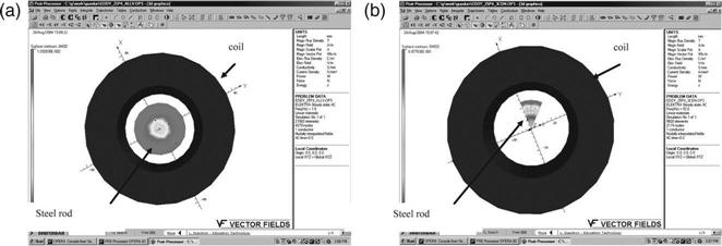
In the EM stress sensor application, if the gradient of the electric current through the primary coil over time is high, the steel cable cannot be uniformly magnetized due to the eddy current, as shown in Fig. 9.20. Through proper design of L-C energizing circuit, the skinning effect can be minimized due to reduced gradient of varying field over time. This effect is simulated by the authors, as indicated in Figs 9.20 and 9.21 in which magnetic flux density in steel cable drops inward axially because of eddy current. More theoretical review and explanation is provided in Reference 35.

9.8 Removable (portable) elastomagnetic stress sensor
Several limitations exist for solenoid-type EM stress sensors. First of all, the solenoid-type sensor is usually designed to be used for ready-to-be-built structures and needs to be installed before the cable is anchored. Although the solenoid sensor can be wound on some existing structures, the calibration procedure is time-consuming. Secondly, the solenoid-type EM sensor is a permanent sensing device, and is not usable once it has been taken down for any reason. Therefore, it is highly desirable to develop a portable and reusable sensor for direct load measurement in steel cable. U-shaped EM sensing technology has been developed and tested in the field. This represents an impressive breakthrough in EM sensing technology.
The U-shaped EM sensor is a magnetic circuit composed of a ferrite yoke and steel rod. It can be used in short and long-term force monitoring. Simulation of magnetic flux is given in Fig. 9.22. More test results are discussed in the References 35 and 36.

The U-shaped yoke, made of grain-oriented silicon steel laminate, can magnetically saturate the cable for stress monitoring of existing cables. The dimensions of the yoke were analyzed for a better magnetization effect. Either the permeability of the steel cable or the flux variation along the circuit reflects the steel stress level. The latter is preferable, due to its total detachability. The load calibration results are shown in Fig. 9.23.

9.9 Conclusion and future trends
Magnetism and magnetoelasticity have been applied in infrastructure health monitoring and inspection. A series of state-of-the-art magnetic and magnetoelastic NDE methods have been reviewed. Recently, EM technology has been used extensively to determine tensile forces of steel cables. The configuration and application of this technology has been described in detail. For future convenient use of EM technology, an innovative removable tensile stress monitoring unit was also developed. This technology will allow widespread use of EM technology in health monitoring of existing structures with various cable systems. Several on-going accomplishments in engineering application of magnetism were described. New and revolutionary magnetic techniques will certainly emerge continually. For example, real-time inspection of transient load in structures through the magnetic method is possible in the very near future. Likewise, in situ corrosion monitoring of steel cables is under extensive study. The final adaptation and field application lie on the development of a product with an integrated and user-friendly package that uses smart algorithm to exclude adverse effects of unrelated noises and interfering factors.