
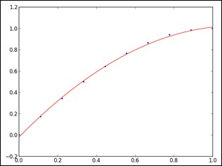
This represents the final result of the method:
For regression from the point of view of curve fitting, there is a generic curve_fit routine in the scipy.optimize module.
This routine minimizes the sum of squares of a set of equations using the Levenberg-Marquardt algorithm and offers a best fit from any kind of functions (not only polynomials or splines). The syntax is simple:
curve_fit(f, xdata, ydata, p0=None, sigma=None, **kw)
The f parameter is a callable function that represents the function we seek, and xdata and ydata are arrays of the same length that contain the x and y coordinates of the points to be fit. The p0 tuple holds an initial guess for the values to be found and sigma is a vector of weights that could be used instead of the standard deviation of the data, if necessary.
We will show its usage with a good example. We will start by generating some points on a section of a sine wave with amplitude A=18, angular frequency w=3π, and phase h=0.5. We corrupt the data in the y array; with some small random noise:
import numpy
import scipy
A=18; w=3*numpy.pi; h=0.5
x=numpy.linspace(0,1,100); y=A*numpy.sin(w*x+h)
y += 4*((0.5-scipy.rand(100))*numpy.exp(2*scipy.rand(100)**2))
We want to estimate the values of A, w, and h from the corrupted data, hence technically finding a curve fit from the set of sine waves. We start by gathering the three parameters in a list and initializing them to some values, for example, A = 20, w = 2π, and h = 1. We also construct a callable expression of the target function (target_function):
import scipy.optimize
p0 = [20, 2*numpy.pi, 1]
target_function = lambda x,AA,ww,hh: AA*numpy.sin(ww*x+hh)
We feed these, together with the fitting data, to curve_fit in order to find the required values:
pF,pVar = scipy.optimize.curve_fit(target_function, x, y, p0)
A sample of pF run on any of our experiments should give an accurate result for the three requested values:
print (pF)
The output for the preceding command is as follows:
[ 18.13799397 9.32232504 0.54808516]
This means that A was estimated to about 18.14, w was estimated very close to 3π, and h was between 0.46 and 0.55. The output of the initial data, together with a computation of the sine wave is as follows, in which original data (in blue on the left-hand side graph), corrupted (in red in both graphs), and computed sine wave (in black in the right-hand side) are shown in the following screenshot:
