
Chapter 54. Introduction to SSAS 2008 data mining
With SQL Server 2008, you get a complete business intelligence (BI) suite. You can use the SQL Server Database Engine to maintain a data warehouse (DW), SQL Server Reporting Services (RS) to create managed and ad hoc reports, SQL Server Integration Services (SSIS) to build and use extract, transform, and load (ETL) applications, and SQL Server Analysis Services (SSAS) to create Unified Dimensional Model (UDM) cubes.
Probably the easiest step into business intelligence is using reports created with RS. But this simplicity has a price. End users have limited dynamic capabilities when they view a report. You can extend the capabilities of RS with report models, but using report models to build reports is an advanced skill for end users. You also have to consider that the performance is limited; for example, aggregating two years of sales data from a production database could take hours. Therefore, RS reports aren’t useful for analyses of large quantities of data over time directly from production systems.
In order to enable end users to do dynamic analysis—online analytical processing (OLAP)—you can implement a data warehouse and SSAS UDM cubes. In addition to dynamic change of view, end users also get lightning-speed analyses. End users can change the view of information in real time, drilling down to see more details or up to see summary information. But they’re still limited with OLAP analyses. Typically, there are too many possible combinations of drilldown paths, and users don’t have time to examine all possible graphs and pivot tables using all possible attributes and hierarchies. In addition, analysts are limited to searching only for patterns they anticipate. OLAP analysis is also usually limited to basic mathematical operations, such as comparing sums over different groups, operations that end users can solve graphically through client tool GUI.
Data mining (DM) addresses most of these limitations. In short, data mining is data-driven analysis. When you create a DM model, you don’t anticipate results in advance. You examine data with advanced mathematical methods, using data mining algorithms, and then you examine patterns and rules that your algorithms find. The SSAS data mining engine runs the algorithms automatically after you set up all of the parameters you need; therefore, you can check millions of different pivoting options in a limited time. In this chapter, you’re going to learn how to perform data mining analyses with SSAS 2008.
Data mining basics
The first question you may ask yourself is what the term data mining means. In short, data mining enables you to deduce hidden knowledge by examining, or training, your data with data mining algorithms. Algorithms express knowledge found in patterns and rules. Data mining algorithms are based mainly on statistics, although some are based on artificial intelligence and other branches of mathematics and information technology as well.
Nevertheless, the terminology comes mainly from statistics. What you’re examining is called a case, which can be interpreted as one appearance of an entity, or a row in a table. The attributes of a case are called variables. After you find patterns and rules, you can use them to perform predictions. In SSAS 2008, the DM model is stored in the SSAS database as a kind of a table. It’s not a table in a relational sense, as it can include nested tables in columns. In the model, the information about the variables, algorithms used, and the parameters of the algorithms are stored. Of course, after the training, the extracted knowledge is stored in the model as well. The data used for training isn’t part of the model, but you can enable drillthrough on a model, and use drillthrough queries to browse the source data.
Most of the literature divides DM techniques into two main classes: directed algorithms and undirected algorithms. With a directed approach, you have a target variable that supervises the training in order to explain its values with selected input variables. Then the directed algorithms apply gleaned information to unknown examples to predict the value of the target variable. With the undirected approach, you’re trying to discover new patterns inside the dataset as a whole, without any specific target variable. For example, you use a directed approach to find reasons why users purchased an article and an undirected approach to find out which articles are commonly purchased together.
You can answer many business questions with data mining. Some examples include the following:
- A bank might ask what the credit risk of a customer is.
- A customer relationship management (CRM) application can ask whether there are any interesting groups of customers based on similarity of values of their attributes.
- A retail store might be interested in which products appear in the same market basket.
- A business might be interested in forecasting sales.
- If you maintain a website, you might be interested in usage patterns.
- Credit card issuers would like to find fraudulent transactions.
- Advanced email spam filters use data mining.
And much, much more, depending on your imagination!
Data mining projects
The Cross-Industry Standard Process for Data Mining (CRISP-DM) defines four main distinct steps of a data mining project. The steps, also shown in figure 1, are as follows:
- Identifying the business problem
- Using DM techniques to transform the data into actionable information
- Acting on the information
- Measuring the result
Figure 1. The CRISP-DM standard process for data mining projects

In the first step, you need to contact business subject matter experts in order to identify business problems. The second step is where you use SQL Server BI suite to prepare the data and train the models on the data. This chapter is focused on the transform step. Acting means using patterns and rules learned in production.
You can use data mining models as UDM dimensions; you can use them for advanced SSIS transformations; you can use them in your applications to implement constraints and warnings; you can create RS reports based on mining models and predictions; and more. After deployment in production, you have to measure improvements of your business. You can use UDM cubes with mining model dimensions as a useful measurement tool. As you can see from figure 1, the project doesn’t have to finish here: you can continue it or open a new project with identifying new business problems.
The second step, the transform step, has its own internal cycle. You need to understand your data; you need to make an overview. Then you have to prepare the data for data mining. Then you train your models. If your models don’t give you desired results, you have to return to the data overview phase and learn more about your data, or to the data preparation phase and prepare the data differently.
Data overview and preparation
Overviewing and preparing the data is probably the most exhaustive part of a data mining project. To get a comprehensive overview of your data, you can use many different techniques and tools. You can start with SQL queries and reports, or you can use UDM cubes. In addition, you can use descriptive statistics such as frequency distribution for discrete variables, and the mean value and the spread of the distribution for continuous variables. You can use Data Source View for a quick overview of your variables in table, pivot table, graph, or pivot graph format. Microsoft Office Excel statistical functions, pivot tables, and pivot graphs are useful tools for data overview as well.
After you understand your data, you have to prepare it for data mining. You have to decide what exactly your case is. Sometimes this is a simple task; sometimes it can get quite complex. For example, a bank might decide that a case for analysis is a family, whereas the transaction system tracks data about individual persons only. After you define your case, you prepare a table or a view that encapsulates everything you know about your case. You can also prepare child tables or views and use them as nested tables in a mining model. For example, you can use an “orders header” production table as the case table, and an “order details” table as a nested table if you want to analyze which products are purchased together in a single order. Usually, you also prepare some derived variables. In medicine, for example, the obesity index is much more important for analyses than a person’s bare height and weight. You have to decide what to do with missing values, if there are too many. For example, you can decide to replace them with mean values. You should also check the outliers—rare and far out-of-bounds values—in a column. You can group or discretize a continuous variable in a limited number of bins and thus hide outliers in the first and the last bin.
SSAS 2008 data mining algorithms
SSAS 2008 supports all of the most popular data mining algorithms. In addition, SSIS includes two text mining transformations. Table 1 summarizes the SSAS algorithms and their usage.
Table 1. SSAS 2008 data mining algorithms and usage
|
Algorithm |
Usage |
|---|---|
|
Association Rules |
The Association Rules algorithm is used for market basket analysis. It defines an itemset as a combination of items in a single transaction; then it scans the data and counts the number of times the itemsets appear together in transactions. Market basket analysis is useful to detect cross-selling opportunities. |
|
Clustering |
The Clustering algorithm groups cases from a dataset into clusters containing similar characteristics. You can use the Clustering method to group your customers for your CRM application to find distinguishable groups of customers. In addition, you can use it for finding anomalies in your data. If a case doesn’t fit well in any cluster, it’s an exception. For example, this might be a fraudulent transaction. |
|
Decision Trees |
Decision Trees is the most popular DM algorithm, used to predict discrete and continuous variables. The algorithm uses the discrete input variables to split the tree into nodes in such a way that each node is more pure in terms of target variable—each split leads to nodes where a single state of a target variable is represented better than other states. For continuous predictable variables, you get a piecewise multiple linear regression formula with a separate formula in each node of a tree. A tree that predicts continuous variables is a Regression Tree. |
|
Linear Regression |
Linear Regression predicts continuous variables, using a single multiple linear regression formula. The input variables must be continuous as well. Linear Regression is a simple case of a Regression Tree, a tree with no splits. |
|
Logistic Regression |
As Linear Regression is a simple Regression Tree, a Logistic Regression is a Neural Network without any hidden layers. |
|
Naïve Bayes |
The Naïve Bayes algorithm calculates probabilities for each possible state of the input attribute for every single state of predictable variable. These probabilities are used to predict the target attribute based on the known input attributes of new cases. The Naïve Bayes algorithm is quite simple; it builds the models quickly. Therefore, it’s suitable as a starting point in your prediction project. The Naïve Bayes algorithm doesn’t support continuous attributes. |
|
Neural Network |
The Neural Network algorithm is often associated with artificial intelligence. You can use this algorithm for predictions as well. Neural networks search for nonlinear functional dependencies by performing nonlinear transformations on the data in layers, from the input layer through hidden layers to the output layer. Because of the multiple nonlinear transformations, neural networks are harder to interpret compared to Decision Trees. |
|
Sequence Clustering |
Sequence Clustering searches for clusters based on a model, and not on similarity of cases as Clustering does. The models are defined on sequences of events by using Markov chains. Typical usage of Sequence Clustering would be an analysis of your company’s website usage, although you can use this algorithm on any sequential data. |
|
Time Series |
You can use the Time Series algorithm to forecast continuous variables. Internally, the Time Series uses two different algorithms. For short-term forecasting, the Auto-Regression Trees (ART) algorithm is used. For long-term prediction, the Auto-Regressive Integrated Moving Average (ARIMA) algorithm is used. You can mix the blend of algorithms used by using the mining model parameters. |
Creating mining models
After a lengthy introduction, it’s time to start with probably the most exciting part of this chapter—creating mining models. By following the instructions, you can create predictive models. You’re going to use Decision Trees, Naïve Bayes, and Neural Network algorithms on the same mining structure. The scenario for these models is based on the AdventureWorksDW2008 demo database. The fictitious Adventure Works company wants to boost bike sales by using a mailing campaign. The new potential customers are in the ProspectiveBuyer table. But the company wants to limit sending leaflets only to those potential customers who are likely to buy bikes. The company wants to use existing data to find out which customers tend to buy bikes. This data is already joined together in the vTargetMail view. Therefore, the data preparation task is already finished, and you can start creating mining models following these steps:
1.
In Business Intelligence Development Studio (BIDS), create a new Analysis Services project and solution. Name the solution and the project TargetMail.
2.
In Solution Explorer, right-click on the Data Sources folder and create a new data source. Use the Native OLE DBSQL Server Native Client 10.0 provider. Connect to your SQL Server using Windows authentication and select the AdventureWorksDW2008 database. Use the Inherit option for the impersonation information and keep the default name, Adventure Works DW2008, for the data source.
3.
Right-click on the Data Source Views folder, and create a new data source view. In the Data Source View Wizard, on the Select a Data Source page, select the data source you just created. In the Select Tables and View pane, select only the vTargetMail view and ProspectiveBuyer table. Keep the default name, Adventure Works DW2008, for the data source view.
4.
Right-click the Mining Structures folder and select New Mining Structure. Walk through the wizard using the following options:
- On the Welcome page of the Data Mining Wizard, click Next.
- In the Select the Definition Method page, use the existing relational database or data warehouse (leave the first option checked).
- In the Create the Data Mining Structure window, in the Which Data Mining Technique Do You Want to Use? drop-down list under the Create Mining Structure with a Mining Model option, select the Decision Trees algorithm from the drop-down list (the default).
- Use Adventure Works DW2008 DSV in the Select Data Source View page.
- In the Specify Table Types page, select vTargetMail as a case table by clicking the Case check box for this table.
5.
By clicking on appropriate check boxes in the Specify the Training Data page, define CustomerKey as a key column (selected by default), BikeBuyer as predictable column, and CommuteDistance, EnglishEducation, EnglishOccupation, Gender, HouseOwnerFlag, MaritalStatus, NumberCarsOwned, NumberChildrenAtHome, Region, and TotalChildren as input columns.
6.
In the Specify Columns’ Content and Data Type page, click the Detect button. The wizard should detect that all columns, except CustomerKey, have discrete content. Note that if you want to use Age and YearlyIncome attributes in the model, you’d have to discretize them if you don’t want a Regression Tree.
7.
In the Create Test Set page, you can specify the percentage of the data or number of cases for the testing set—the holdout data. Use the default splitting, using 30 percent of data as the test set. You’ll use the test set to evaluate how well different models perform predictions.
8.
Type TM as the name of the mining structure and TM_DT as the name of the model in the Completing the Wizard page.
9.
Click Finish to leave the wizard and open the Data Mining Designer. Save the project.
You’re going to add two models based on the same structure. In Data Mining Designer, select the Mining Models tab. To add a Naïve Bayes model, right-click on TM_DT, and then select the New Mining Model option. Type TM_NB as the name of the model and select the Microsoft Naive Bayes algorithm. Click OK.
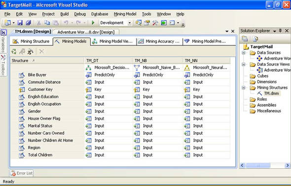
To add a Neural Network model, right-click the TM_DT model and again select the New Mining Model option. Type TM_NN as the name of the model and select the Microsoft Neural Network algorithm. Click OK. Save, deploy, and process the complete project. Don’t exit BIDS. Your complete project should look like the one in figure 2.
Figure 2. Predictive models project
Harvesting the results
You created three models, yet you still don’t know what additional information you got, or how you can use it. In this section, we’ll start with examining mining models in BIDS, in the Data Mining Designer, with the help of built-in Data Mining Viewers. The viewers show you patterns and rules in an intuitive way. After the overview of the models, you have to decide which one you’re going to deploy in production. We’ll use the Lift Chart built-in tool to evaluate the models. Finally, we’re going to simulate the deployment by creating a prediction query. We’ll use the Data Mining Extensions (DMX) language with a special DMX prediction join to join the mining model with the ProspectiveBuyer table and predict which of the prospective customers is more likely to buy a bike.
Viewing the models
To make an overview of the mining models, follow these steps:
1.
In BIDS, in the Data Mining Designer window, click the Mining Model Viewer tab. If the TM_DT model isn’t selected by default in the Mining Model drop-down list on the top left of the window, select it.
2.
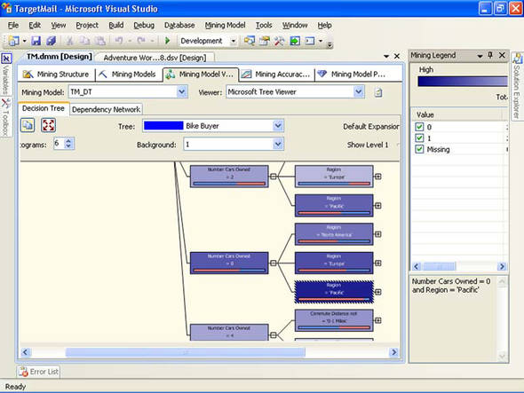
Verify that you have the Decision Tree tab open. In the Background drop-down list, select value 1 of the Bike Buyer to check the potential buyers only. We’re not interested in groups of customers that aren’t going to buy a bike. Note the color of the nodes: the darker the color is, the more bike buyers appear in the node. For example, the node that groups people for whom the Number Cars Owned attribute is equal to 0 and Region is Pacific is quite dark in color. Therefore, the potential bike buyers are in that node. From the Mining Legend window, you can see more detailed information: more than 91 percent of people in this node have bought a bike in the past. You can see this information shown in figure 3.
Figure 3. Decision tree
3.
In the Dependency Network viewer, use the slider on the left side of the screen to show the strongest links only. Try to identify the two variables with the highest influence on the Bike Buyer attribute.
4.
Navigate to the Mining Model Viewer tab and select the TM_NB model to view the model that uses the Naïve Bayes algorithm.
5.
The first viewer is the Dependency Network viewer. Does the Naïve Bayes algorithm identify the same two variables as having the highest influence on the Bike Buyer attribute? Different algorithms make slightly different predictions.
6.
Check other Naïve Bayes viewers as well. The Attribute Discrimination viewer is useful: it lets you see the values of input attributes that favor value 1 of the Bike Buyer attribute and the values that favor value 0.
7.
Check the Neural Network model. The only viewer you’ll see is the Attribute Discrimination viewer, in which you can again find the values of input attributes that favor value 1 of the Bike Buyer attribute and those values that favor value 0. In addition, you can filter the viewer to show the discrimination for specific states of input attributes only.
Evaluating the models
As you probably noticed, different models find slightly different reasons for customers’ decisions whether to buy a bike. The question is how you can evaluate which model performs the best. The answer is quite simple in SQL Server 2008. Remember that when you created the models, you split the data into training and test sets. The model was trained on the training set only; you can make the predictions on the test set. Because you already know the outcome of the predictive variable in the test set, you can measure how accurate the predictions are. A standard way to show the accuracy is the Lift Chart. You can see a Lift Chart created using the data and models from this section in figure 4.
Figure 4. Lift Chart for models created in this section

In figure 4, you’ll notice five curves and lines on the chart; yet, you created only three models. The three curves show the performance of the predictive models you created, and the two lines represent the Ideal Model and the Random Guess Model. The x axis shows the percentage of population (all cases), and the y axis shows the percentage of the target population (bike buyers in this example). The Ideal Model line (the topmost line) shows that approximately 50 percent of the customers of Adventure Works buy bikes. If you want to know exactly who’s going to buy a bike and who isn’t, you’d need only 50 percent of the population to get all bike buyers. The lowest line is the Random Guess line. If you picked cases out of the population randomly, you’d need 100 percent of the cases for 100 percent of bike buyers. Likewise, you’d need 80 percent of the population for 80 percent of bike buyers, 60 percent of the population for 60 percent of bike buyers, and so on. The mining models you created give better results than the Random Guess Model, and of course worse results than the Ideal Model. In the Lift Chart, you can see the lift of the mining models from the Random Guess line; this is where the name Lift Chart comes from. Any model predicts the outcome with less than 100 percent of probability in all ranges of the population; therefore, to get 100 percent of bike buyers, you still need 100 percent of the population. But you get interesting results somewhere between 0 and 100 percent of the population. For example, with the best-performing model in this demo case, the line right below the Ideal Model line, you can see that if you select 70 percent of the population based on this model, you’d get nearly 90 percent of bike buyers. You can see in the Mining Legend window that this is the Decision Trees model. Therefore, in this case, you should decide to deploy the Decision Trees model into production.
In order to create a Lift Chart, follow these steps:
1.
In BIDS, in the Data Mining Designer, click the Mining Accuracy Chart tab.
In the Input Selection window, make sure that all three mining models are selected in the Select Predictable Mining Model Columns to Show in the Lift Chart table and that the Synchronize Prediction Columns and Values check box is checked. Also make sure that in the Select Data Set to Be Used for Accuracy Chart option group, the Use Mining Model Test Cases option is selected. Leave the Filter expression box empty.
2.
In the Predict Value column of the Select Predictable Mining Model Columns to Show in the Lift Chart table, select 1 in the drop-down list of any row. We’re interested in showing the performance of the models when predicting positive outcome—when predicting buyers only.
3.
Click the Lift Chart tab. Examine the Lift Chart. Don’t exit BIDS.
Creating prediction queries
Finally, it’s time to select probable buyers from the ProspectiveBuyer table. You can do this task with a DMX prediction join query. Detailed description of the DMX language is out of scope for this book. Fortunately, you can get a jump start with the Prediction Query builder in BIDS. A similar builder is included in the RS Report Designer when you’re authoring a report based on a data mining model, and in SSIS Package Designer in the Data Mining Query task and Data Mining Query transformation. In order to create a DMX prediction query in BIDS, follow these steps:
1.
In the Data Mining Designer, select the Mining Model Prediction tab.
2.
In the Select Model window, select the best-performing model. In this case, this is the Decision Trees model, which should be selected by default, as it was the first model created.
3.
In the Select Input Table(s) window, click on the Select Case table button. Select the ProspectiveBuyer table. Click OK.
4.
Check the join between model and table; it’s done automatically based on column names. You can change the join manually, though following a consistent naming convention is a good practice.
5.
In the bottom pane, define the column list of your DMX Select statement.
6.
In the Source and Field columns, select the following attributes: Prospective-BuyerKey, FirstName, and LastName, from the ProspectiveBuyer table, and Bike Buyer from the TM_DT mining model. Your selections in the Prediction Query builder should look like the selections in figure 5.
Figure 5. Prediction Query builder

7.
In the Switch to Query Result drop-down list, accessed through the leftmost icon on the toolbar, select the Query option. Check the DMX query created.
8.
In the Switch to Query Result drop-down list, select the Result option. In the result table, you can easily notice who’s going to buy a bike and who isn’t, according to the Decision Trees prediction.
9.
Save the project and exit BIDS.
Sources for more information
You can learn more about data mining using SQL Server 2008 Books Online, SQL Server Analysis Services—Data Mining section (http://msdn.microsoft.com/en-us/library/bb510517.aspx).
For a complete overview of the SQL Server 2008 BI suite, refer to the MCTS Self-Paced Training Kit (Exam 70-448): Microsoft SQL Server 2008—Business Intelligence Development by Erik Veerman, Teo Lachev, and Dejan Sarka (MS Press, 2009).
An excellent guide to SSAS data mining is Data Mining with Microsoft SQL Server 2008 by Jamie MacLennan, ZhaoHui Tang, and Bogdan Crivat (Wiley, 2008).
You can find a lot of additional information, tips, and tricks about SSAS data mining at the SQL Server Data Mining community site at http://www.sqlserverdatamining.com/ssdm/default.aspx.
If you’re interested in Cross-Industry Standard Process for Data Mining (CRISP-DM), check the CRISP-DM site at http://www.crisp-dm.org/index.htm.
Summary
Data mining is the most advanced tool in the BI suite. Data mining projects have a well-defined lifecycle. Probably the most exhaustive part of the project is the data preparation and overview. With SSAS 2008, you can quickly create multiple models and compare their performance with standard tools such as Lift Chart. In addition, you can create DMX prediction queries through a graphical query builder. SQL Server 2008 includes all of the most popular data mining algorithms.
All elements of the SQL Server 2008 BI suite are interleaved; it’s easy to use one element when creating another. For example, you can create mining models on SQL Server databases and Analysis Services UDM cubes; you can deploy a mining model as a new dimension in a SSAS UDM cube; and you can use mining models in RS reports and SSIS packages.
About the author

Dejan Sarka focuses on developing database and business intelligence applications. Besides projects, he spends about half of his time on training and mentoring. He’s a frequent speaker at some of the most important international conferences. He’s the founder of the Slovenian SQL Server and .NET Users Group. As lead author or coauthor, Dejan has written seven books about SQL Server. Dejan Sarka has also developed two courses for Solid Quality Mentors: Data Modeling Essentials and Data Mining with SQL Server.