
CHAPTER 13
Parameter Analysis of the VPIN (Volume-Synchronized Probability of Informed Trading) Metric
Jung Heon Song
Kesheng Wu
Horst D. Simon
Lawrence Berkeley National Lab
INTRODUCTION
The Flash Crash of 2010
The May 6, 2010, Flash Crash saw the biggest one-day point decline of 998.5 points (roughly 9 percent) and the second largest point swing of 1,010.14 points in the Dow Jones Industrial Average. Damages were also done to futures trading, with the price of the S&P 500 decreasing by 5 percent in the span of 15 minutes, with an unusually large volume of trade conducted. All of these culminated in market value of $1 trillion disappearing, only to recover the losses within minutes—20 minutes later, the market had regained most of the 600 points drop (Lauricella 2011). Several explanations were given about the market crash. Some notable ones are:
- Phillips (2010) listed a number of reports, which pointed out that the Flash Crash was a result of a fat-finger trade in Procter & Gamble, leading to a massive stop-loss orders (this theory, however, was quickly dismissed, as the Procter & Gamble incident came about after much damage had already been done to the E-mini S&P 500).
- Some regulators attributed it to high-frequency traders for exacerbating pricing. Researchers at Nanex argued that quote stuffing—placing and then immediately canceling a large number of rapid-fire orders to buy or sell stocks—forced competitors to slow down their operations (Bowley 2010).
- The Wall Street Journal reported a large purchase of put options by the hedge fund Universa Investments, and suggested that this might have triggered the Flash Crash (Lauricella and Patterson 2010).
- Flood (2010) attributed technical difficulties at the NY Stock Exchange (NYSE) and ARCA to the evaporation of liquidity.
- A sale of 75,000 E-mini S&P 500 contracts by Waddell & Reed might have caused the futures market to collapse (Gordon and Wagner 2010).
- Krasting (2010) blamed currency movements, especially a movement in the U.S. dollars to Japanese yen exchange rate.
After more than four months of investigation, the U.S. Securities and Exchange Commission (SEC) and Commodity Futures Trading Commission (CFTC) issued a full report on the Flash Crash, stating that a large mutual fund firm's selling of an unusually large number of E-Mini S&P 500 contracts and high-frequency traders’ aggressive selling contributed to the drastic price decline of that day (Goldfarb 2010).
VPIN: A Leading Indicator of Liquidity-Induced Volatility
A general concern in most of these studies is that the computerized high frequency trading (HFT) has contributed to the Flash Crash. It is critical for the regulators and the market practitioners to better understand the impact of high frequency trading, particularly the volatility. Most of the existing market volatility models were developed before HFT had widely been used. We believe that disparities between traditional volatility modeling and high-frequency trading framework have led to the difficulty in CFTC's ability to understand and regulate the financial market. These differences include new information arriving at irregular frequency, all models that seek to forecast volatility treating its source as exogenous, and volatility models being univariate as a result of exogeneity (López de Prado 2011).
A recent paper by Easley, Lopez de Prado, and O'Hara (2012) applies a market microstructure model to study behavior of prices a few hours before the Flash Crash. The authors argue that new dynamics in the current market structure culminated to the breakout of the event and introduced a new form of probability of informed trading—volume synchronized probability of informed trading (VPIN)—to quantify the role of order toxicity in determining liquidity provisions (Easley, López de Prado, O'Hara 2011).
The paper presents an analysis of liquidity on the hours and days before the market collapse, and highlights that even though volume was high and unbalanced, liquidity remained low. Order flow, however, became extremely toxic, eventually contributing to market makers leaving the market, causing illiquidity.
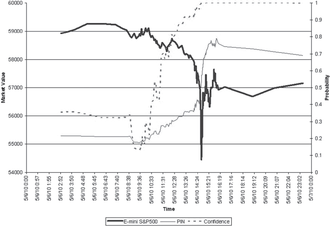
Figure 13.1 shows the VPIN values of E-mini futures during the day of the Flash Crash. Near 11:55 A.M. on May 6, the value of VPIN exceeded 90 percent threshold value, and around 1:08 P.M., it passed 95 percent. The VPIN value attained its maximum by 2:30 P.M., and the market crash starts to occur at 2:32 P.M., which agrees with the CFTC/SEC report. This and other tests on different trading instruments provide anecdotal evidences that VPIN is effective.
Systemic Validation of VPIN
To explore whether VPIN is effective in a generic case, one needs to define an automated testing mechanism and execute it over a large variety of trading instruments. To this end, Wu, Bethel, Gu, Leinweber, and Rüebel (2013) adopted a simple definition for VPIN events. A VPIN event starts when the VPIN values cross over a user-defined threshold from below and last for a user-defined fixed duration. We also call each event a VPIN prediction, during which we expect the volatility to be higher than usual. If the volatility is indeed above the average of randomly selected time intervals of the same duration, we say that the event is a true positive; otherwise, it is labeled as a false positive. Alternatively, we may also say that the prediction is a true prediction or a false prediction. Given these definitions, we can use the false positive rate (FPR) to measure the effectiveness of VPIN predictions. Following the earlier work by López de Prado (2012), Wu, Bethel, Gu, Leinweber, and Rüebel (2013) chose to use an instantaneous volatility measure called Maximum Intermediate Return (MIR) to measure the volatility in their automated testing of effectiveness of VPIN.
In order to apply VPIN predictions on a large variety of trading instruments, Wu, Bethel, Gu, Leinweber, and Rüebel (2013) implemented a C++ version of the algorithm. In their test involving 97 most liquid futures contracts over a 67-month period, the C++ implementation required approximately 1.5 seconds for each futures contract, which is many orders of magnitude faster than an alternative. This efficient implementation of VPIN allows them to examine the effectiveness of VPIN on the largest collection of actual trading data reported in literature.
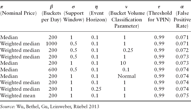
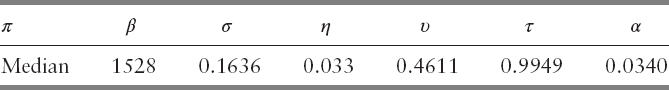
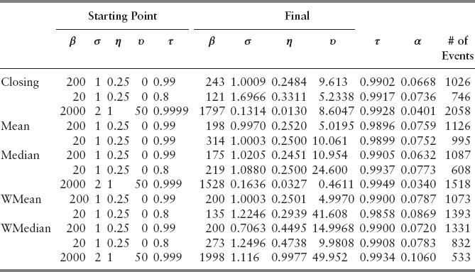
The VPIN predictions require the user to set a handful of different parameters, such as the aforementioned threshold on VPIN values and duration of VPIN events. The choices of these free parameters can affect FPR, the measured effectiveness of VPIN predictions. The authors computed the number of VPIN events and number of false positive events, and used FPR as the effectiveness score for VPIN predictions. The computation of VPIN involves a number of free parameters that must be provided by the users. For each of these parameter choices, the average FPR value over all 97 futures contracts was computed. After examining 16,000 parameter combinations, the authors found a collection of the parameter combinations that can reduce the average false positive rates from 20 percent to 7 percent. The best of these parameter combinations are shown in Table 13.1. We will provide definitions of the parameters as we describe the details of VPIN computation in the next section.
From Table 13.1, we see that these parameter combinations differ from each other in many ways, making it difficult to provide a concise recommendation on how to set these free parameters of VPIN. This chapter attempts a more systematic search of the parameter space. We plan to accomplish this goal in two steps: parameter optimization and sensitivity analysis. First, we search for the optimal parameters with a popular optimization library NOMAD (Nonlinear Mesh Adaptive Direct Search) by Audet, Le Digabel, and Tribes (2009), and Le Digabel (2011). Once the parameters with the minimal FPR values are found, we carry out sensitivity analysis using an uncertainty quantification software package named UQTK (Uncertainty Quantification Toolkit) by Sargsyan, Safta, Debusschere, and Najm (2012).
DEFINITION OF VPIN
Based on an idealized trading model shown in Figure 13.2, Easley, Kiefer, O'Hara, and Paperman (1996) defined a way to measure the information imbalance from the observed ratio of buys and sells in the market. The authors termed the measure probability of informed trading and used PIN as the shorthand. To compute PIN, one classifies each trade as either buy or sell, following some classification rule (Ellis, Michaely, O'Hara 2000), bins the trades buckets, and then calculates the relative difference between the buys and sells in each bucket. The probability of informed trading is the average buy–sell imbalance over a user-selected time window, which we will call the support window. This support window is typically expressed as the number of buckets.

In their analysis of the Flash Crash of 2010, Easley, López de Prado, and O'Hara (2011) proposed grouping the trades into equal volume bins and called the new variation the volume synchronized probability of informed trading (VPIN). The new analysis tool essentially stretches out the busy periods of the market and compresses the light trading periods. The authors termed this new virtual timing measure the volume time. Another important parameter in computing VPIN is the number of buckets per trading day.
An important feature in computing the probability of informed trading is that it does not actually work with individual trades, but, rather, with groups of bars, treating each as if it is a single trade. The trade classification is performed on the bars instead of actual trades. Both bars and buckets are forms of binning; the difference is that a bar is smaller than a bucket. A typical bucket might include tens or hundreds of bars. Based on earlier reports, we set the number of bars per bucket to 30 for the remainder of this work, as it has minor influence on the final value of the VPIN as shown from the published literature (Easley, López de Prado, O'Hara 2012; Abad, Yague 2012).
The price assigned to a bar is called the nominal price of the bar. This is a second free parameter for VPIN. When the VPIN (or PIN) value is high, we expect the volatility of the market to be high for a certain time period. To make this concrete, we need to choose a threshold for the VPIN values and a size for the time window.
Following the notation used by Wu, Bethel, Gu, Leinweber, and Rüebel (2013), we denote the free parameters needed for the computation of the VPIN as follows:
- Nominal price of a bar π
- Parameter for the bulk volume classification (BVC) ν
- Buckets per day (BPD) β
- Threshold for VPIN τ
- Support window σ
- Event horizon η
Next, we provide additional details about these parameters.
Pricing Strategies
VPIN calculations are typically performed in time bars or volume bars. The most common choice of nominal price of a bar used in practice is the closing price—that is, the price of the last trade in the bar. In this work, we consider the following five pricing options for our analysis: closing prices, unweighted mean, unweighted median, volume-weighted mean, and volume-weighted median.
Bulk Volume Classification
A common method used to classify a trade as either buyer-initiated or seller-initiated is via the tick rule, or more formally, the Lee-Ready trade classification algorithm. The method assigns a trade as buy if its price is higher than the preceding, and as sell if otherwise. This convention depends on the sequential order of trades, which is not the ideal approach in high-frequency trading. Instead, the bulk volume classification (BVC) assigns a fraction of the volume to buys and the rest to sells based on the normalized sequential price change (Easley, López de Prado, and O'Hara 2012). Let ![]() denote the buy volume for bar j, and the volume of bar to be Vj. We follow the definitions by Easley, López de Prado, and O'Hara (2012) for the computation of
denote the buy volume for bar j, and the volume of bar to be Vj. We follow the definitions by Easley, López de Prado, and O'Hara (2012) for the computation of ![]() :
:
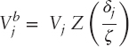
where Z denotes the cumulative distribution function of either the normal or the student t-distribution, ζ the standard deviation of {δj}, where δj = Pj − Pj−1, {Pj} are the prices of a sequence of volume bars. We also denote the degrees of freedom of Z by υ, and in the case of the standard normal distribution, we let υ = 0. The rest of the volume bar is then considered as sells
![]()
Even though this formula uses a cumulative distribution function, it does not imply that the authors have assumed this distribution has anything to do with the actual distribution of the data. The actual empirical distribution of the data has been used, but according to Easley, López de Prado, and O'Hara (2012) no improvement was seen in empirical testing. We decided to use the BVC for its computational simplicity and, as noted by Easley, López de Prado, and O'Hara (2012), its accuracy, which parallels those of other commonly used classification methods.
The argument of the function Z can be interpreted as a normalizer of the price changes. In a traditional trading model, the average price change is subtracted first before dividing by the standard deviation. In HFT, however, the mean price is much smaller than the standard deviation ζ (Wu, Bethel, Gu, Leinweber, Ruebel 2013). We make use of the results from earlier works by Easley, López de Prado, and O'Hara (2012) by always using zero as the center of the normal distribution and the student-t distribution.
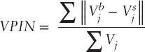
By definition, only the most recent few buckets are needed for the computation of the VPIN value (Easley, Kiefer, O'Hara, Paperman, 1996). We call this the support window, represent it as a fraction of the number of buckets in a day, and denote it by σ. The formula used to compute the VPIN is (Easley, López de Prado, O'Hara 2012)
Following the works of earlier authors, we normalize the VPIN values by working with the following transformation:

where erf is the error function measured by a normal distribution, μ the mean of the VPIN values, σ the standard deviation.
VPIN Event
If the value x is a normal distribution with mean μ and standard deviation σ, then the value Φ(x) denotes the fraction of values that are less than the specific value. This is a useful transformation, as it transforms the value of x from an open range to a close range between 0 and 1. The transformation allows using a single threshold τ for a variety of different trading instruments convenient. For example, in earlier tests, Easley, López de Prado, and O'Hara (2011; 2012) typically used the value 0.9 as the threshold for Φ(x). Had the VPIN values followed the normal distribution, this threshold would have meant that a VPIN event is declared when a VPIN rises above 90 percent of the values. One might expect that 10 percent of the buckets will produce VPIN values above this trigger. If one divides a day's trading into 100 buckets, one might expect 10 of the buckets to have VPIN values greater than the threshold, which would produce too many VPIN events to be useful. However, Wu, Bethel, Gu, Leinweber, and Rüebel (2013) reported seeing a relatively small number of VPIN events—about one event every two months. The reason for this observation is the following. First off, the VPIN values do not follow the normal distribution. The above transformation is a convenient shorthand for selecting a threshold, not an assumption or validation that VPIN values follow the normal distribution. Furthermore, we only declare a VPIN event if Φ(x) reaches the threshold from below. If Φ(x) stays above the threshold, we will not declare a new VPIN event. Typically, once Φ(x) reaches the threshold, it will stay above the threshold for a number of buckets; thus, many large Φ(x) values will be included in a single VPIN event. This is another way that the VPIN values do not follow the normal distribution.
Our expectation is that immediately after a VPIN event is triggered, the volatility of the market would be higher than normal. To simplify the discussion, we declare the duration of a VPIN event to be η days. We call this time duration the event horizon for the remainder of the discussion.
False Positive Rate
After we have detected a VPIN event, we next determine if the given event is a true positive or a false positive. As indicated before, we use MIR to measure the volatility. Since the MIR can be both positive and negative, two separate average MIR values are computed: one for the positive MIR and one for the negative MIR. These two values then establish a normal range. If the MIR of a VPIN event is within this normal range, then it is a false event; otherwise, it is a true event. We denote the false positive rate by α, where α is
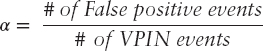
The flowchart in Figure 13.3 summarizes how a VPIN event is classified. When the number of VPIN events triggered is 0, the above formula is ill defined. To avoid this difficulty, when no event is detected, we let the number of false positive events to be 0.5 and the number of events 0.5 as well, hence FPR = 1.
To quantify the effectiveness of VPIN, we compute the average false positive rate over the 97 most active futures contracts from 2007 to 2012. For each futures contract, we compute the VPIN values to determine the number of VPIN events and number of false positive events. The average FPR reported later is the ratio between the total number of false positive events and the total number of events. Note that we are not taking average of FPRs of different futures contracts to compute the overall FPR. Assuming that each time a VPIN that crosses the threshold from below signals an opportunity for investments—a true event leads to a profitable investment and a false positive event leads to a losing investment—the FPR we use is the fraction of “losing” investments. Thus, the overall FPR we use is a meaningful measure of the effectiveness of VPIN.
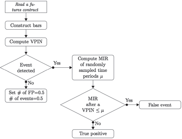
FIGURE 13.3 Flowchart of how a VPIN event is classified.
Source: Wu, Bethel, Gu, Leinweber, Rüebel 2013
COMPUTATIONAL COST
From our tests, we observe that reading the futures contracts and constructing bars are one of the most time-consuming steps within the algorithm. For example, an analysis on the computation of VPIN on nine metal futures contracts over the 67-month period shows that reading the raw data took 11.93 percent of the total time, and constructing the bars took 10.35 percent, while the remaining computation required 10.59 percent second. In addition, we ranked the computational cost of each parameter in VPIN. Results show that the construction of the bars is the most time consuming, followed by bucket volume classification, evaluation of VPIN, transformation of VPIN using the error function, and calculation of MIR value—that is, β > ν > σ > τ > η.
To reduce the computational cost, the data are read into memory, and the computations are arranged so that the constructed bars are stored in memory. This allows all different computations to be preformed on the bars, with reading the original data again. Furthermore, we arrange our computations so that the intermediate results are reused as much as possible. For example, the same VPIN values can be reused when we change the threshold for event triggers and the event horizon. This knowledge is particularly useful for efficiently testing the sensitivity of the parameters (we need to calculate VPIN values of a large number of points to construct the surrogate model to be later used in sensitivity analysis).
Figure 13.4 shows a breakdown of time needed to construct volume bars with different pricing options. We see that for the weighted median, it requires as much as seven times more time than those of closing, mean, and weighted mean, and for median, as much as five times more.
To better take advantage of the multiple cores in a typical CPU, we implemented multithreaded program to compute false positive rate for each contract independently. Our tests are performed on an IBM DataPlex machine at the NERSC, which imposes a maximum run time of single computational job of 72 hours. For almost all tests, our program terminated in less than 72 hours. For those that did not terminate within the time limitation, we restart the test program using the latest values of the free parameters as their new starting points. Although this approach does succeed in finding the optimal solution, it loses track of the computational history, and therefore the overall optimization process is not as efficient as if we had run through the whole test without interruption. This restart requires more computation time, but should not have affected the final answers we have found.
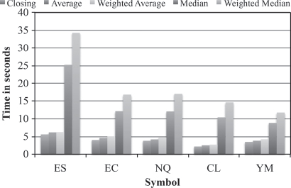
FIGURE 13.4 Time (seconds) needed to construct volume bars with different nominal prices.
Source: Wu, Bethel, Gu, Leinweber, Rüebel 2013
OPTIMIZATION OF FPR
The main goal of an optimization software is solving problems of the form
![]()
where Ω is a subset of n-dimensional space with constraints denoted by cj. The dual of this problem, finding the maximum, can be easily computed by multiplying the objective function by −1. There are many ways to numerically solve an optimization. For simple linear programming, the simplex method is available. For nonlinear problems, one approach is via iterative methods. Depending on the nature of the objective function, specifically differentiability, one can select from a number of existing algorithms.
Popular iterative methods that make use of derivative (or by approximation through finite differences) include quasi-Newton, conjugate gradient, and steepest-descent methods. A major advantage of using the derivatives is improved rate of convergence. There are also well-known software packages such as L-BFGS that implement quasi-Newton methods to solve large-scale optimization problems (Nocedal, Liu 1989).
In the computation of VPIN, the relationship between the free parameters and the final FPR values is defined through a lengthy computation procedure. There is no obvious ways to evaluate whether a small change in any of the parameters will produce small changes in FPR. For such a nonsmooth objective function, approximation of its derivative may not lead to desirable answers. The computational cost of optimization algorithms designed to work without a derivative can also vary greatly from one problem to another. In this case, a successful search strategy is via generalized pattern search (GPS) (Audet, Béchardand, Le Digabel 2008). We say a problem is a blackbox problem if either the objective function(s) or constraints do not behave smoothly. The MADS algorithm (Audet, Dennis 2006) is an extension of the GPS algorithm (Torczon, 1997; Audet, Dennis 2003), which is itself an extension of the coordinate search (Davidon 1991). NOMAD is a C++ implementation of MADS algorithm designed for constrained optimization of a blackbox problem. In this chapter, we deliberately chose NOMAD, as it not only extends the MADS algorithm to incorporate various search strategies, such as VNS (variable neighborhood search), to identify the global minimum of the objective function(s) (Audet, Béchardand, Le Digabel 2008), but also targets blackbox optimization under general nonlinear constraints.
MADS (Mesh Adaptive Direct Search) Algorithm
The main algorithm utilized in NOMAD is the MADS (Audet, Le Digabel, Tribes 2009; Le Digabel 2011), which consists of two main steps: search and poll. During the poll step, it evaluates the objective function f and constraints cj at mesh points near the current value of xk. It generates trial mesh points in the vicinity of xk. It is more rigidly defined than the search step, and is the basis of the convergence analysis of the algorithm (Audet, Le Digabel, and Tribes 2009). Constraints can be blackboxes, nonlinear inequalities, or Boolean. As for x, it can also be integer, binary, or categorical (Le Digabel 2011). Readers interested in detailed explanation on how different constraints and x are treated can refer to Le Digabel (2011).
The MADS algorithm is an extension of the GPS algorithm for optimization problems, which allows polling in a dense set of directions in the space of variables (Audet, Dennis 2008). Both algorithms iteratively search for a solution, where the blackbox functions are repeatedly evaluated at some trial points. If improvements are made, they are accepted, and rejected if not. MADS and GPS generate a mesh at each iteration, and it is expressed in the following way (Audet, Béchardand, and Le Digabel 2008):
![]()
where Vk denotes the collection of points evaluated at the start of kth iteration, Δk ∈ ![]() + the mesh size parameter, and D a constant matrix with rank n. D is, in general, simply chosen to be an orthogonal grid of In augmented by −In, that is, [In − In]. The poll directions are not a subset of this matrix D, and can still have much flexibility. This is why no more complicated D is used. For readers interested in a detailed discussion of the algorithm, see the paper by Audet, Béchardand, and Le Digabel (2008).
+ the mesh size parameter, and D a constant matrix with rank n. D is, in general, simply chosen to be an orthogonal grid of In augmented by −In, that is, [In − In]. The poll directions are not a subset of this matrix D, and can still have much flexibility. This is why no more complicated D is used. For readers interested in a detailed discussion of the algorithm, see the paper by Audet, Béchardand, and Le Digabel (2008).
The search step is crucial in practice for its flexibility, and has the potential to return any point on the underlying mesh, as long as the search does not run into an out-of-memory error. Its main function is narrowing down and searching for a point that can improve the current solution.
Figure 13.5 shows the pseudocode of the MADS algorithm.
NOMAD Optimization Results
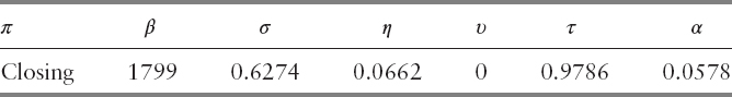
Although NOMAD can solve minimization problem involving categorical variables, doing so will significantly reduce the efficiency of the algorithm for this particular case. A breakdown of time needed to construct volume bars with different pricing options shows that weighted median is the most computationally heavy pricing option, with closing price located at the opposite end of the spectrum. Each pricing strategy was considered separately to reduce the amount of time needed for each run of the program submitted to the computer. This arrangement also reduces the complexity of understanding of the parameter space and allows for obtaining a better solution set. Solutions obtained from different starting points are shown in Table 13.4. The optimal parameter combination from Table 13.4 is


However, varying initial choices of the parameters under the same pricing strategy is shown to be inconsistent, which suggests that the global optimal solution might still be out of reach. We attempted to reach this global optimal solution by enabling the variable neighborhood search (VNS) strategy.
Variable Neighborhood Search (VNS) Strategy
The VNS is a metaheuristic strategy proposed by Mladenović and Hansen (1997) for not only solving global optimization problems, but also combinatorial problems. It incorporates a descent method and a neighborhood structure to systematically search for the global minimum. For an initial solution x, the descent method searches through a direction of descent from x with respect to the neighborhood structure N(x), and proceeds to find the minimum of f(x) within N(x). This process is repeated until no improvement is possible.
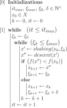
The neighborhood structure could play a critical role in finding the global optimum. VNS makes use of a random perturbation method when the algorithm detects it has found a local optimum. This perturbed value generally differs to a large extent so as to find an improved local optimum and escape from the previous localized subset of Ω. The perturbation method, which is parameterized by a non-negative scalar ξk, depends heavily on the neighborhood structure. The order of the perturbation, ξk, denotes the VNS amplitude at kth iteration. Figure 13.6 succinctly summarizes the algorithm into two steps: the current best solution is perturbed by ξk, and VNS performs the descent method from the perturbed point. If an improved solution is discovered, it replaces the current best solution, and ξk is reset to the initial value. If not, a non-negative number δ (the VNS increment) is added to ξk, and resumes the descent method. This process is repeated until ξk reaches/exceeds a maximum amplitude ξmax (Audet, Le Digabel, and Tribes 2009; Audet Béchardand, Le Digabel 2008; Mladenović, and Hansen 1997).
VNS in NOMAD
The VNS algorithm is incorporated in NOMAD as a search step (called the VNS search). If no improvement is achieved during MADS's iteration, new trial points are created closer to the poll center. The VNS, however, focuses its search on a distant neighborhood with larger perturbation amplitude. Since the poll step remains the same, as long as the following two conditions are met, no further works are needed for convergence analysis (Audet, Béchardand, and Le Digabel 2008).
- For each ith iteration, all the VNS trial points must be inside the mesh M(i,Δi).
- Their numbers must be finite.
To use VNS strategy in NOMAD, the user must define a parameter that sets the upper bound for the number of VNS blackbox evaluations. This number, called VNS_SEARCH, is expressed as the ratio of VNS blackbox evaluations to the total number of blackbox evaluations. The default value is 0.75 (Audet, Le Digabel, and Tribes 2009).
VNS Optimization Results
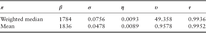
Table 13.5 shows a collection of optimization results with VNS strategy enabled. The two lowest FPRs obtained are 2.44 percent and 2.58 percent, using the following parameter set, respectively.
Even though the improvement is a mere 1 percent, these data sets are much more valuable for practical uses (especially the second set). The number of events detected for
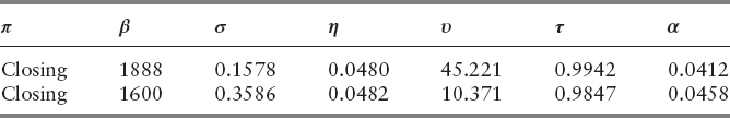
is 1518, whereas those for the two sets in Table 13.2 are 2062 and 2298. These two sets convey improved accuracy and precision. Furthermore, the second set of Table 13.2 detected more VPIN events than the first and is computationally more efficient. Given the difference in FPR is minimal, is more suited to be used in practice. Even so, VNS strategy failed to address the divergence of FPR when different starting parameters are chosen. We attempted to resolve this issue by increasing both the maximum blackbox evaluations and VNS_SEARCH (Table 13.3).

These two sets were both found with maximum blackbox evaluations of 5,000 and VNS_SEARCH = 0.75. However, no direct correlation of the values of these parameters with consistent FPR was observed. Maximum blackbox evaluations was set to 6,000 and VNS_SEARCH = 0.85. Yet, NOMAD returned FPR that is inferior to the two above.
From Table 13.5, we observe that the majority of FPR falls consistently within the range of 3 percent to 5 percent. Even though the optimization procedure consistently produces parameter combinations that give us FPR between 3 percent and 5 percent, the parameter values are actually different. Our next task is to understand the sensitivity of these parameter choices, that is, how the different parameter choices affect our effectiveness measure, FPR (Table 13.4).
UNCERTAINTY QUANTIFICATION (UQ)
In many cases of mathematical modeling, we do not have complete knowledge of the system or its intrinsic variability. These uncertainties arise from different places such as parameter uncertainty, model inadequacy, numerical uncertainty, parametric variability, experimental uncertainty, and interpolation uncertainty (Kennedy and O'Hagan 2001). Therefore, even if the model is deterministic, we cannot rely on a single deterministic simulation (Le Maître and Knio 2010). We must, therefore, quantify the uncertainties through different methods. Validation of the surrogate model and analysis of variance are frequently used to carry out UQ and sensitivity analysis.

Validation involves checking whether the surrogate model constructed from the original model correctly represents our model. Analysis of variance provides users with important information relevant to design and optimization. The user can identify the controllability of the system, as measured through sensitivity analysis, and characterize the robustness of the prediction (Najm 2009). There are two ways to approach UQ: forward UQ and inverse UQ. UQTK makes use of the former to perform its tasks.
UQTK
A UQ problem involves quantitatively understanding the relationships between uncertain parameters and their mathematical model. Two methodologies for UQ are forward UQ and inverse UQ. The spectral polynomial chaos expansion (PCE) is the main technique used for forward UQ. First introduced by Wiener (1938), polynomial chaos (PC) determines evolution of uncertainty using a nonsampling based method, when there is probabilistic uncertainty in the system parameters. Debusschere, Najm, Pébay, Knio, Ghanem, and Le Maître (2004) note advantages to using a PCE:
- Efficient uncertainty propagation
- Computationally efficient global sensitivity analysis
- Construction of an inexpensive surrogate model, a cheaper model that can replace the original for time-consuming analysis, such as calibration, optimization, or inverse UQ
We make use of the orthogonality and structure of PC bases to carry out variance-based sensitivity analysis.
From a practical perspective, understanding how the system is influenced by uncertainties in properties is essential. One way of doing so is through analysis of the variance (ANOVA), a collection of statistical models that analyzes group mean and variance. The stochastic expansion of the solution provides an immediate way to characterize variabilities induced by different sources of uncertainties. This is achieved by making use of the orthogonality of the PC bases, making the dependency of the uncertain data and model solution obvious.
The Sobol (or the Hoeffding) decomposition of any second-order deterministic functional f allows for expressing the variance of f in the following way (Le Maître and Knio 2010)

where ![]() . Since
. Since ![]() contributes to the total variance among the set of random parameters {xi, i ∈ s}, this decomposition is frequently used to analyze the uncertainty of the model. Then for all s ∈ {1,…, N}, we can calculate sensitivity indices as the ratio of the variance due to xi, Vi(f), to V(f), such that summing up the indices yields 1 (Le Maître and Knio 2010).
contributes to the total variance among the set of random parameters {xi, i ∈ s}, this decomposition is frequently used to analyze the uncertainty of the model. Then for all s ∈ {1,…, N}, we can calculate sensitivity indices as the ratio of the variance due to xi, Vi(f), to V(f), such that summing up the indices yields 1 (Le Maître and Knio 2010).

The set {Ss} is Sobol sensitivity indices that are based on variance fraction—that is, they denote fraction of output variance that is attributed to the given input.
UQTK first builds quadrature using a user-specified number of sampled points from each parameter. For each controllable input, we evaluate it with each point of the quadrature to construct PCE for the model. Next, we create the surrogate model and conduct global sensitivity analysis using the approach just described.
UQ Results
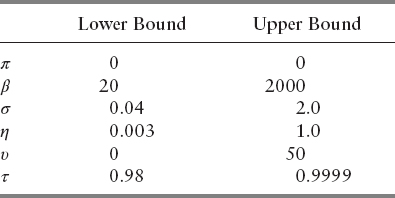
Based on the formulation of VPIN, it can be readily understood that the objective function behaves smoothly with respect to the CDF threshold, τ. The higher the cutoff, the smaller the number of events detected. The objective function must behave smoothly with respect to its controllable input, so we conducted sensitivity analysis with τ as the controllable input, consisting of 19 equidistant nodes in the corresponding interval of Table 13.6. The quadrature is generated by taking samples of five points from each of β, σ, η, and υ. The pricing strategy used here is closing, and this is for practical reasons: Wu, Bethel, Gu, Leinweber, and Rüebel reported in 2013 relative computational costs for five largest futures contracts with different nominal prices, ranking weighted median, median, weighted average, average, and closing in descending order (see Figure 13.4). Because these five futures contracts (S&P 500 E-mini, Euro FX, Nasdaq 100, Light Crude NYMEX, and Dow Jones E-mini) constitute approximately 38.8 percent of the total volume, closing price will still be the most efficient strategy for our data set. In addition, many high-frequency traders opt to use closing price in their daily trading.
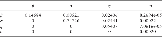
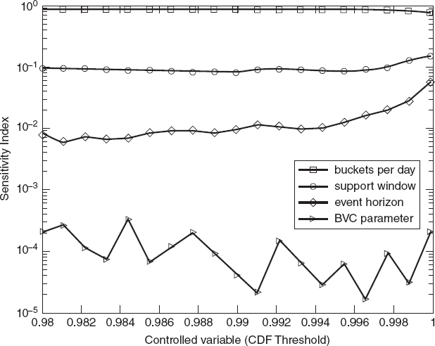
From Table 13.7, β and σ are the two most influential parameters. Sobol index of υ is reasonable as well, given no uniform behavior of υ was observed from outputs of NOMAD and Wu's paper. We interpret these numbers in the following way: Assuming the inputs are uniformly distributed random variables over their respective bounds, then the output will be a random uncertain quantity whose variance fraction contributions are given in Table 13.7 by Sobol indices. We then plot the semilog of the indices for each value of CDF threshold (Figure 13.7).
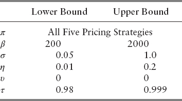
We see from Figure 13.7 consistent Sobol indices of BPD and its dominance over those of other parameters. The indices of support window and event horizon do behave similarly until τ ≈ 1, at which point we observe sudden fluctuation of the numbers. This is largely due to abnormal behavior of the objective function when the CDF threshold is close to 1. If we set the threshold too high, only a small fraction of events will be detected, in which case the objective function would return high FPR (refer to Figure 13.4). Hence, the anomaly is not too unreasonable. The plot also shows a nonuniform behavior of BVC parameter's Sobol indices. In addition, its contribution to overall sensitivity is minimal. When the degree of freedom (υ) for the Student's t-distribution is large enough, the t-distribution behaves very much like the standard normal distribution. Figure 13.7 shows minimal sensitivity from BVC parameter. As such, we let υ = 0 for the remainder of our studies for computational simplicity. In order to see the sensitivity due to τ and how the model behaves with different π, we set π to be the controllable input and changed the bounds to reflect more practical choices of the parameters.
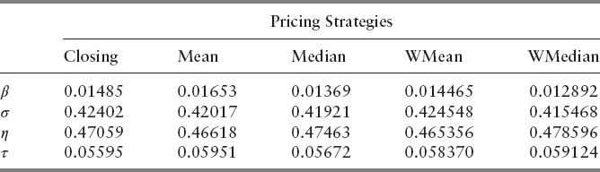
Even though π is a categorical variable, it is used here as the index at which the sensitivities are computed. The controllable input is a way to index multiple sensitivity analysis being performed at once—that is, the controllable input can be the x location where we compute the sensitivities of the observable of interest, or it could be the index of the categorical value at which we want to get the sensitivities, or it could even be the index of multiple observables in the same model for which we want sensitivities. As such, using π as the controllable input does not bar us from carrying out sensitivity analysis (Tables 13.8, 13.9).
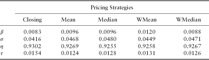
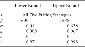
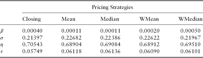
We then made the mesh even finer by setting the lower and upper bounds to include the majority of output parameters found in Table 13.5. The ranges are shown in Table 13.10. We sought to find out which parameter is the most influential one in these bounds. From Table 13.11, we see that no other parameters except η behave in a volatile way. As these bounds did not provide much insight to other variables, we changed the bounds so that they correspond to the parameters of the lowest FPRs. Ranges are specified in Table 13.12. The Sobol indices in Table 13.13 tell us that β and τ become insignificant when they are chosen in these intervals. σ and η, however, are extremely volatile, and most responsible for the variance of the objective function. We see from Table 13.11 and 13.13 that pricing options play minimal role in contributing to the overall sensitivity. Within the bounds prescribed in Table 13.10 and 13.12, it is suggested that the user select closing, unweighted mean, or weighted mean for computational efficiency.
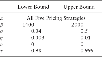
The sensitivity analysis tells us that the range of each parameter we specify affects each one's relative importance. Initially, the support window and buckets per day were the dominant variables. As we made the mesh finer and changed it to correspond to the best results from NOMAD, we see that the event horizon and the support window become the determining parameters that control the variance of the objective function. This indicates that when the number of buckets per day is between 1600 and 1888, and the VPIN threshold is between 0.97 and 0.998, their exact values have little influence on the resulting FPR.
CONCLUSION
We have analytically explored the parameter space of VPIN by rigorously searching for the global minimum FPR and conducting sensitivity analysis on a number of parameter bounds. Although we were not successful in finding the global minimizer of FPR, our test results from VNS optimization displayed some degree of consistency.
To better understand the parameter choices, we used uncertainty quantification to analyze the objective function's sensitivity with respect to each parameter. Results indicate oscillatory behavior of BVC parameter and minimal fluctuations observed in buckets per day, support window, and event horizon for τ not too close to 1. Studying changes in variance under different pricing strategies informed us that within the bounds obtained from NOMAD output, they play minimal role in determining the FPR.
From our analysis, we suggest using the following ranges of parameters for practical applications of VPIN:
- Using the mean price within a bar as the nominal price for the bar. Computing mean is quite efficient. Although there was little to no variation when using other pricing options, mean did yield one of the lowest FPRs.
- Sensitivity analysis shows the contribution from buckets per day is negligible when its values are between 1600 and 1800. We suggest using a number that lies in an interval of about 1836.
- Support window is an important parameter. Even a small perturbation can cause a drastic difference in FPR. We suggest the user to use a number very close to 0.0478.
- Event horizon is another important variable to consider. Like support window, it is highly volatile. We suggest the user to use 0.0089.
- CDF threshold is important. However, the analysis shows that as long as we are working with τ > 0.98, its influence becomes minimal (but it should never be too close to 1).
Easley, López de Prado, and O'Hara (2010) stated some potential applications of the VPIN metric:
- Benchmark for execution brokers filling their customers’ orders. The clients can also monitor their brokers’ actions and measure how effectively they avoided adverse selection.
- A warning sign for market regulators who can regulate market activity under different flow toxicity level.
- An instrument for volatility arbitrage.
We believe that results from our optimization and sensitivity analysis can aid in improving the efficiency of the VPIN metric.
Acknowledgments: We would like to thank the Department of Energy's Workforce Development of Teachers and Scientists as well as Workforce Development and Education at Berkeley Lab for initially supporting this research. We would also like to thank Dr. Bert Debusschere for his help with UQTK.
REFERENCES
Abad, D., and J. Yague. 2012. From PIN to VPIN: An introduction to order flow toxicity. The Spanish Review of Financial Economics 10 (2):74–83.
Audet, C., V. Béchardand, and S. Le Digabel. 2008. Nonsmooth optimization through mesh adaptive direct search and variable neighborhood search. Journal of Global Optimization 41 (2): 299–318.
Audet, C., S. Le Digabel, and C. Tribes. 2009. NOMAD user guide. Technical Report G-2009–37.
Audet, C., and J. E. Dennis Jr., 2006. Mesh adaptive direct search algorithms for constrained optimization. SIAM Journal on Optimization 17 (1): 188–217.
_________. 2003. Analysis of generalized pattern searches. SIAM Journal on Optimization, 13 (3): 889–903.
Bowley, G. 2010. Lone $4.1 billion sale led to “Flash Crash” in May. The New York Times.
_________. 2010. Stock swing still baffles, ominously. The New York Times.
Debusschere, B. J., H. N. Najm, P. P. Pébay, O. M. Knnio, R. G. Ghanem, and O. P. Le Maître. 2004. Numerical challenges in the use of polynomial chaos representations for stochastic processes. SIAM J. Sci. Comp. 26 (2): 698–719.
Easley, D., N. M. Kiefer, M. O'Hara, and J. B. Paperman. 1996. Liquidity, information, and infrequently traded stocks. The Journal of Finance 51 (4): 1405–1436.
Easley, D., M. López de Prado, and M. O'Hara. 2011. The microstructure of the “Flash Crash”: Flow toxicity, liquidity crashes and the probability of informed trading. Journal of Portfolio Management 37 (2): 118–128.
_________. 2012. Flow toxicity and liquidity in a high frequency world. Review of Financial Studies 25 (5): 1457,1493.
_________. 2012. The Volume Clock: Insights into the High Frequency Paradigm. http://ssrn.com/abstract=2034858.
Ellis, K., R. Michaely, and M. O'Hara. 2000. The accuracy of trade classification rules: Evidence from NASDAQ. Journal of Financial and Quantitative Analysis.
Flood, J. 2010. NYSE confirms price reporting delays that contributed to the Flash Crash. AI5000.
Goldfarb, Z. 2010. Report examines May's Flash Crash, expresses concern over high-speed trading. The Washington Post.
Gordon, M., and D. Wagner. 2010. “Flash Crash” report: Waddell & Reed's $4.1 billion trade blamed for market plunge. Huffington Post.
Kennedy, M., and A. O'Hagan. 2001. Bayesian calibration of computer models. Journal of the Royal Statistical Society. Series B Volume 63, Issue 3.
Krasting, B. 2010. The yen did it. Seeking Alpha.
Lauricella, T. 2010. Market plunge baffles Wall Street—Trading glitch suspected in “mayhem” as Dow falls nearly 1,000, then bounces. The Wall Street Journal, p. 1.
Lauricella, T., and S. Patterson. 2010. Did a big bet help trigger “black swan” stock swoon? The Wall Street Journal.
Lauricella, T., K. Scannell, and J. Strasburg. 2010. How a trading algorithm went awry. The Wall Street Journal.
Le Digabel, S. 2011. Algorithm 909: NOMAD: Nonlinear optimization with the MADS algorithm. ACM Transactions on Mathematical Software 37 (4): 44:1–44:15.
Le Maître, O., P. Knio, and M. Omar. 2010. Spectral Methods for Uncertainty Quantification: With Applications to Computational Fluid Dynamics (Scientific Computation), 1st ed. New York: Springer.
López de Prado, M. 2011. Advances in High Frequency Strategies. Madrid, Complutense University.
Mladenović, N., and P. Hansen. 1997. Variable neighborhood search. Computers and Optimization Research 24 (11): 1097–1100.
Najm, H. N. 2009. Uncertainty quantification and polynomial chaos techniques in computational fluid dynamics. Annual Review of Fluid Mechanics 41: 35–52.
Nocedal, J., and D. C. Liu. 1989. On the Limited Memory for Large Scale Optimization. Mathematical Programming B 45 (3): 503–528.
Phillips, M. 2010. SEC's Schapiro: Here's my timeline of the Flash Crash. The Wall Street Journal.
Sargsyan, K., C. Safta, B. Debusschere, and H. Najm. 2012. Uncertainty quantification given discontinuous model response and a limited number of model runs. SIAM Journal on Scientific Computing 34 (1): B44–B64.
Wiener N. 1938. The homogeneous chaos. American Journal of Mathematics 60 (4): 897–936.
Wu, Ke., W. Bethel, M. Gu, D. Leinweber, and O. Ruebel. 2013. A big data approach to analyzing market volatility. Algorithmic Finance 2 (3-4): 241–267.