
CHAPTER 14
Covariance Specification Tests for Multivariate GARCH Models1
Charles F. Dolan School of Business, Fairfield University
INTRODUCTION
Proper modeling of the variances and covariances of financial assets is extremely important for many reasons. For example, risk premia are typically a function of risk that is mostly measured by the variance or the covariance of the asset of interest with some market index. Similarly, risk management requires the use of the variance–covariance matrix of portfolios of risky assets.
Recently, research interest has focused on the time variability of variances and covariances with the use of ARCH-type models. The autoregressive conditionally heteroskedastic model (ARCH) was proposed by Engle (1982) as a way of modeling volatility clustering. Even though the model was originally applied to UK unemployment data, it has been particularly successful in the modeling of variances of financial time series. There is a plethora of applications of univariate ARCH-type models in the area of finance (see Bollerslev, Chou, and Kroner 1992, for an excellent survey). Bollerslev, Engle, and Wooldridge (1988) introduced and estimated the first multivariate GARCH class of models. Koutmos and Booth (1995) introduced a multivariate exponential GARCH model to study volatility spillovers across major national stock markets.
The class of ARCH-type models has been extremely useful in terms of accommodating various hypotheses as well as stylized facts observed in financial time series. Consequently, there have been several versions of these models at both the univariate and the multivariate level (see for example Andersen et al. 2006). Such variety, however, created the need to discriminate among different versions in terms of how well they fit the data. To facilitate the model selection process Engle and Ang (1993) introduced a series of diagnostics based on the news impact curve implied by the particular ARCH model used. The premise is that if the volatility process is correctly specified, then the squared standardized residuals should not be predictable on the basis of observed variables. Using these tests, we can determine how well the particular model captures asymmetries in the variance, and how well it accommodates large negative and positive innovations.
These tests have been proven very useful and easy to implement. However, there has been no similar set of tests to evaluate the performance of multivariate versions of ARCH-type models. In this chapter, I propose a set of covariance diagnostics along the lines of Engle and Ng (1993). These diagnostics can guide the researcher in terms of the appropriateness of the particular specification for the covariance function. Such diagnostics are essential for multivariate ARCH models, especially since in many instances the various covariance specifications cannot be nested making it impossible to use nested hypotheses testing to decide among models.
The rest of this chapter is organized as follows: First is the description of the covariance specification tests and the estimation procedures, followed by a comparison of three covariance specifications using standard traditional tests as well as the proposed covariance specification tests.
COVARIANCE SPECIFICATION TESTS
The volatility specification tests proposed by Engle and Ng (1993) can be described by the following set of equations:
where εt and σt are the estimated residuals and the standard deviations from the particular ARCH type model used, zt = εt/σt are the standardized residuals, S−t−1 is a dummy variable that takes the value of unity if εt−1 is negative and zero otherwise, and et is an error term. The premise is that if the volatility process is correctly specified, then the squared standardized residuals should not be predictable on the basis of observed variables.
The first test examines the impact of positive and negative innovations on volatility not predicted by the model. The squared residuals are regressed against a constant and the dummy S−t−1. The test is based on the t-statistic for S−t−1. The negative size bias test examines how well the model captures the impact of large and small negative innovations. It is based on the regression of the standardized residuals against a constant and S−t−1εt−1. The calculated t-statistic for S−t−1εt−1 is used in this test. The positive sign bias test examines possible biases associated with large and small positive innovations. Here, the standardized filtered residuals are regressed against a constant and (1 − S−t−1)εt−1. Again, the t-statistic for (1 − S−t−1)εt−1 is used to test for possible biases. Finally, the joint test is an F-test based on a regression that includes all three variables; that is, S−t−1, S−t−1εt−1, and (1 − S−t−1)εt−1.
As mentioned earlier, even though these diagnostics are applied routinely to determine the fit of volatility models, they provide no evidence regarding the fit of covariance models in the case of multivariate ARCH models. As such, I propose extending the Engle and Ng (1993) tests to the specification of the covariance function. The idea is that if the covariance of the returns of two assets i and j is correctly specified, then information regarding the past sign and size of the innovations of the two assets should not be able to predict the product of cross-standardized residuals.
Let ξi,j,t = (εi,t/σi,t)(εj,t/σj,t) be the product of standardized residuals, S−i,t a dummy that takes the value of 1 if εi,t < 0 and zero otherwise and S−j,t a dummy that takes the value of 1 if εj,t < 0 and zero otherwise. The proposed tests can then be based on the following regressions:


If the covariance model is correctly specified, then we should expect the coefficients in regressions above to be jointly zero. Thus, individual t-tests and/or F-tests could be used to test the null hypothesis of correct specification. Given that these are multivariate regressions, the F-statistics is more appropriate.
APPLICATION OF COVARIANCE SPECIFICATION TESTS
In this section, I estimate a bivariate GARCH model with three different covariance specifications. The bivariate model used can be described by the following set of equations:
where, ri,t and rj,t are the continuously compounded returns on assets i and j; μi,t and μj,t are the conditional means; ![]() ,
, ![]() are the conditional variances; and εi,t and εj,t are innovations or error terms. Equations (14.11) and (14.12) specify the conditional volatility along the lines of a standard GARCH(1,1) process amended by the terms δiSi,t−1ε2i,t−1 and δjSj,t−1ε2j,t−1 where, Sk,t−1 = 1 if εk,t−1 < 0 and zero otherwise for k = i, j. These terms are designed to capture any potential asymmetry in the conditional variance (see Glosten, Jagannathan, and Runkle 1989). Such asymmetries have been attributed to changes in the financial leverage so much so that asymmetric volatility has been termed the leverage effect, even though such an explanation is not very convincing (see, e.g., Bekaert and Wu 2000; Koutmos 1998; and Koutmos and Saidi 1995).
are the conditional variances; and εi,t and εj,t are innovations or error terms. Equations (14.11) and (14.12) specify the conditional volatility along the lines of a standard GARCH(1,1) process amended by the terms δiSi,t−1ε2i,t−1 and δjSj,t−1ε2j,t−1 where, Sk,t−1 = 1 if εk,t−1 < 0 and zero otherwise for k = i, j. These terms are designed to capture any potential asymmetry in the conditional variance (see Glosten, Jagannathan, and Runkle 1989). Such asymmetries have been attributed to changes in the financial leverage so much so that asymmetric volatility has been termed the leverage effect, even though such an explanation is not very convincing (see, e.g., Bekaert and Wu 2000; Koutmos 1998; and Koutmos and Saidi 1995).
Completion of the system requires that the functional form of the covariance be specified. I use three alternative specifications for the purpose of applying the cross-moment tests discussed earlier. It should be pointed out that in the context of the bivariate model the cross-moment is simply the covariance. The three alternative covariance specifications are as follows:
The first model (14.13a) is the constant correlation model introduced by Bollerslev (1990). This model assumes that the conditional correlation ρi,j is constant. It has been used extensively in the literature, especially for large-scale systems because of its simplicity. Model (14.13b) is the vector GARCH model introduced by Bollerslev, Engle, and Wooldridge (1988). It models the covariance as function of the product of past innovations and past covariances. It has more flexibility because it allows for a time varying conditional correlation. Model (14.13c) is the asymmetric vector GARCH model. It is basically an extended version of (14.13b), where the extension consists of allowing the covariance to respond asymmetrically to past innovations from assets i and j in which Si,t−1 and Sj,t−1 are dummy variables taking the value of 1 if the corresponding past innovations are negative and zero otherwise.
The bivariate GARCH model is estimated allowing alternatively the covariance to follow (14.13a), (14.13b), and (14.13c). Subsequently the residuals from the three models are subjected to the covariance specification diagnostics.
EMPIRICAL FINDINGS AND DISCUSSION
The data set used to estimate the three versions of the model are the returns of the stock market portfolio (U.S. market index) and the returns of the portfolio of the banking sector. The data are obtained from the data library of professor Kenneth French (http://mba.tuck.dartmouth.edu/pages/faculty/ken.french/data_library.html).
The market index is value weighted and includes all firms listed in the NYSE, AMEX, and Nasdaq. The sample period extends from January 2, 1990, until December 31, 2013, for a total of 6,048 daily observations. Table 14.1 presents some basic diagnostics on the standardized residuals obtained by the three models. The variance ratio tests are based on the notion that the forecast of a variable should have a lower variance than the variable itself; see Shiller (1981). For example, σ2i,t is the conditional forecast of ε2i,t. Therefore, the variance of σ2i,t should be smaller than the variance of ε2i,t. Similarly, σi,j,t is the conditional forecast of εi,tεm,t. Therefore, Var(σi,j,t) < Var(εi,tεj,t). On these tests, there is no evidence of misspecification in the variance or the covariance functions across all three models. Likewise, the Ljung–Box statistics shows no evidence of autocorrelation in the cross product of standardized residuals for the vector GARCH and the asymmetric vector GARCH models. It does show significant autocorrelation in the case of the constant correlation model, suggesting that this particular specification fails to capture persistence in the covariance.

Though the above tests are very useful, they are not designed to capture asymmetries and nonlinearities in the covariance. For this we turn to the estimated covariance specification tests discussed earlier.
Table 14.2 reports the covariance specification tests. The results are rather interesting. Looking at the constant correlation model, it can be seen that this particular covariance specification fails to capture the sign of positive and negative residuals (sign bias test). Simply put, the covariance exhibits a type of asymmetry that the model fails to capture. Also, the model fails to capture the size of negative residuals as can be seen by the negative size bias test. The joint test also rejects the hypothesis that the product of standardized residuals cannot be predicted using past information.
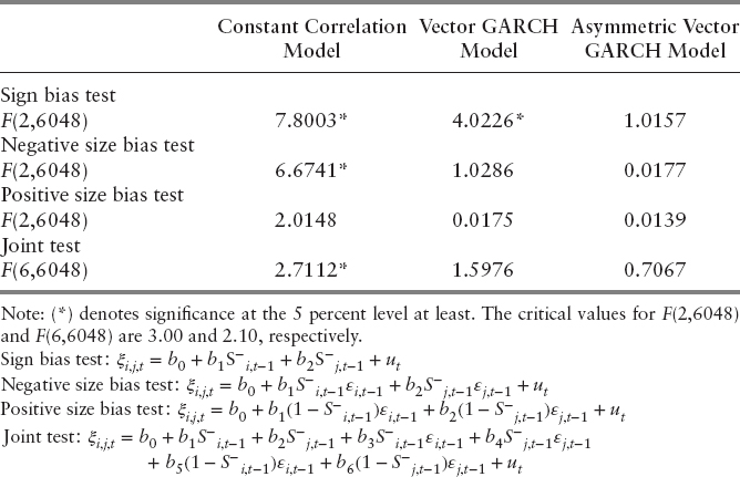
Moving on to the vector GARCH model, the evidence suggests that the covariance specification fails that sign bias test, but it passes the rest of the tests. These findings point in the direction of using a covariance specification that is capable of capturing asymmetry. This conclusion is supported by the evidence regarding the asymmetric vector GARCH model. The covariance specification tests fail to reject the hypothesis that the sign and the size of past residuals cannot be used to better predict the conditional covariance.
It should be pointed out that in this particular application, the covariance models used were nested so that other tests can also be used, in addition to the covariance tests. The advantage of the proposed covariance tests, however, is that they can be applied equally well in cases were competing models are not nested.
CONCLUSION
This paper proposes a set of covariance specification tests analogous to the tests suggested by Engle and Ang (1993) for the conditional variance. The tests are applied to a bivariate model, with three possible covariance specifications. The tests allow the researcher to discriminate among competing hypotheses regarding the covariance, whether the models are nested or not. Since efficient covariance estimates are important for pricing and risk-managing portfolios, these tests could provide additional information and guidance in the process of selecting the appropriate covariance models in different applications.
REFERENCES
Andersen, T. G., T. Bollerslev, P. F. Christoffersen, and F. X. Diebold. 2006. Volatility and correlation forecasting. In Handbook of Economic Forecasting, edited by G. Elliot, C. W. J. Granger, and A. Timmermann, 778–878. Amsterdam: North-Holland.
Bekaert, G., and G. Wu. 2000. Asymmetric volatility and risk in equity markets. The Review of Financial Studies 13: 1–42.
Bollerslev, T. 1990. Modeling the coherence in short-run nominal exchange rates: A multivariate generalized ARCH model. Review of Economics and Statistics 72: 498–505.
Bollerslev, T., R. Y. Chou, and K. F. Kroner. 1992. ARCH modeling in finance: A review of the theory and empirical evidence. Journal of Econometrics 52: 5–59.
Bollerslev, T., R. Engle, and J. M. Wooldridge. 1988. A capital asset pricing model with time varying covariance. Journal of Political Economy 96: 116–131.
Engle, R. F. 1982. Autoregressive conditional heteroskedasticity with estimates of the variance of U.K. inflation. Econometrica 50: 286–301.
Engle, R. F., and V. K. Ang. 1993. Measuring and testing the impact of news on volatility. Journal of Finance 48: 1749–1778.
Glosten, L., R. Jagannathan, and D. Runkle. 1989. Relationship Between the Expected Value and the Volatility of the Nominal Excess Return on Stocks, Working paper, Department of Finance, Columbia University.
Koutmos, G., and G. G. Booth. 1995. Asymmetric volatility transmission in international stock markets. Journal of International Money and Finance 14: 55–69.
Koutmos, G., and R. Saidi. 1995. The leverage effect in individual stocks and the debt to equity ratio. Journal of Business Finance and Accounting 22: 1063–1075.
Koutmos, G. 1998. Asymmetries in the conditional mean and the conditional variance: Evidence from nine stock markets. Journal of Economics and Business 50: 277–290.
_________. 1999. Cross-Moment Specification Tests. Working paper, Charles F. Dolan School of Business, Fairfield University.
Shiller, R. 1981. Do prices move too much to be justified by subsequent changes in dividends? American Economic Review 71: 421–435.