
CHAPTER 4
A Practical Guide to Regime Switching in Financial Economics
Leeds University, UK
Mark Freeman
Loughborough University, UK
David Hillier
University of Strathclyde, UK
Malcolm Kemp
Nematrian Limited, UK
Qi Zhang
Leeds University, UK
A standard assumption in empirical finance is that logarithmic returns to a number of financial asset classes are independently and identically normally distributed (i.i.n.d.). This is convenient to work with analytically and underlies a number of the key theorems in asset pricing, including the Black–Scholes–Merton options pricing model. A further assumption is also commonly invoked that restricts the correlations between different financial assets to be constant over time. This, again, aids in determining closed-form solutions to optimal asset allocation problems.
Despite the mathematical appeal of this framework, it is well known that it does not accurately capture the real-world dynamics of asset returns. There are extensive literatures that document time-varying expected returns, time-varying volatility (heteroskedasticity), autocorrelation, fat-tailed distributions where outliers occur considerably more frequently than might be estimated under the assumption of normality (leptokurtosis), and time-variation in cross-sectional correlation when describing the actual price behavior of financial assets.
Markov regime switching models are one of a range of statistical techniques that capture these observed characteristics of asset returns in a manageable and easily interpretable way. In the next section we provide a brief overview of Markov regime switching models in an academic setting; we then go on to describe the basic mathematical properties of these models in the case when there is only a single asset as well as extending this to multiple assets before considering more complex calibrations. Finally, we look at the use of Markov models and the challenges that can occur in using these models in practice.
A BRIEF LOOK AT MARKOV REGIME SWITCHING IN ACADEMIC ECONOMICS AND FINANCE
This first section of this chapter is intended to provide a brief overview of the applicability of and contexts in which academic research in economics and finance has applied Markov regime switching models. Since Hamilton (1988) and Schwert (1989), the literature has grown exponentially with ever more sophisticated techniques being applied across a multitude of economic and financial settings. The following gives an indication of just how wide the range of settings in which regime switching has been effectively utilized in economic analysis: stock returns (e.g., Ang and Baekert, 2002a); exchange rate dynamics (e.g., Dahlquist and Gray, 2000); interest rates (e.g., Sims and Zha, 2006); option pricing (Boyle and Draviam, 2007); bond pricing (Elliot and Siu, 2009); and pension fund solvency (Abouraschi et al., 2014).
Interestingly, in his comprehensive review of the use of Markov regime switching in empirical finance, Guidolin (2012) finds that in choosing to employ a regime-switching framework for economic analysis, around 50 percent of papers use regime switching because of statistical considerations—that is, the use of a regime-switching framework is dictated by the data. The other 50 percent, however, pick a regime-switching framework on the basis of economic considerations (e.g., analyzing the business cycle). As Guidolin (2012) notes, these two differing approaches, therefore, lead to two very different types of paper. The first is a traditional horse race where regime-switching models are pitched against other types of modeling—for example, regime switching versus a linear benchmark model. The second are papers that are firmly rooted in economic theory.
Markov switching models are well suited to the analysis of economic and financial time series. Since Hamilton's (1989) paper analyzing the business cycle in the United States, the idea that such models can analyze different states, such as expansion and recession, around a long-run trend clearly corresponds to the actual experience of most economies. Crucially, regime-switching models, therefore, have an intuitive interpretation. Moreover, as Ang and Timmerman (2011) note, in the context of financial time series, identified regimes correspond to distinct states such as differing regulatory periods or changes to policy. Further, such models introduce the ability to capture extreme market movements, which is a common feature in financial time-series. Regime switch models are, therefore, suitable for analyzing a wide range of data in the presence of fat tails, skewness, and time-varying correlations.
Further, one of the standard assumptions of finance and asset pricing, as demonstrated by the Capital Asset Pricing Model, is that risk-return payoffs are positive and linear in a monotonic fashion. However, this once again does not correspond to real-life experience. Markets can remain flat for prolonged periods; markets can crash and remain low; or they can grow for sustained periods. Experience has shown repeatedly that the economy can be in a “good” state or a “bad” state (e.g., a boom or a bust). This links to the idea that the economy, or a market for that matter, can be in a period that has more certain, and by definition, more stable return growth, or it can be in a period of high uncertainty where returns are increasingly uncertain. Such differential risk-return trade-offs occur as a consequence of time-varying consumption growth (Whitelaw, 2000). From the point of view of investors, this introduces an additional risk that they may wish to manage when optimizing their portfolio, as the existence of “good” and “bad” regimes, which result in non-monotonic asset returns, increases uncertainty, even if portfolios are largely in the more stable “normal” regime (Ang and Timmerman, 2011).
As noted earlier there are a wide range of applications and settings in which regime switching can be utilized. We, therefore, focus, albeit briefly, on three key areas of academic interest within the regime-switching literature, namely, interest rates, exchange rates, and stock returns and asset allocation.
REGIME SWITCHING AND INTEREST RATE PROCESSES
We first focus on interest rate processes, as this is where the application of regime switching was first utilized by Hamilton (1988) in the analysis of the term structure of interest rates. A key finding of this research is that interest rate regimes are closely related to differing monetary policy regimes (Hamilton, 1988; Sola and Driffill, 1994; Bekaert et al., 2001; and Ang and Bekaert (2002b and 2002c). Such findings clearly show the applicability of regime-switching modeling to such a setting as one would fully expect interest rates to be linked to different monetary policy regimes. Moreover, prior research has shown that interest rate dynamics are related to inflation expectations (Evans and Wachtel, 1993); real interest rates (Garcia and Perron, 1996); and inflation risk premiums (Ang et al. 2008).
Within this area, the work of Ang et al. (2008) is of particular note. Prior research into interest rate regimes had only considered one factor, such as inflation expectations. As such, the analysis would examine states of high inflation, low inflation, deflation, and the probability of being in a given inflationary state. However, in their 2008 model, Ang et al. incorporate two inflationary regimes and two real rate determinants. Moreover, unlike prior research into the inflation risk premium—for example, Campbell and Viceira (2001) that considered a single regime with a constant inflation risk premium—Ang et al. (2008) incorporate a time-varying inflation risk premium into a four-state regime model. Their results show that, in general, real short-term interest rates for the United States are low (circa 1.3 percent) and inflation is high; however, neither interest rates nor inflation exhibit large amounts of volatility.
Consistent with the idea that regime-switching models capture shifts in policy, the results of Ang et al. (2008), found an increasing frequency of regimes with decreasing inflation in the United States. As they note, these regimes are characterized by a downward-sloping real yield curve and swift decreases in inflation, and are consistent with activist monetary policy, which increases real interest rates at the short end of the yield curve. Moreover, these results are in line with Clardia et al. (2000), Boivin (2006), and Cho and Moreno (2006), who demonstrated a structural break in U.S. monetary policy during in the post-Volker period.
REGIME SWITCHING AND EXCHANGE RATES
As with other financial time series, exchange rates follow long-run trends that have periods of very high short-term volatility (Ang and Timmermann, 2011). Consistent with prior literature in interest rate dynamics, such changes have been attributed to underlying government policy with regards to foreign exchange. For example, Froot and Obstfeld (1991) implement dynamic regime switching models for three scenarios where the government will restrict a currency float within a specific range; peg a currency at a specified future level; or unify a system of dual exchange rates. In considering these three policies, they show that regime-switching models are well specified for capturing such dynamics. Similarly, regime switching has been used by Dahlquist and Gray (2000) to examine the European Monetary System (EMS), and they identified periods where currencies were weak and defended against speculation via interest rates, and periods where currencies were stronger and were characterized by a free-float.
The applicability of regime-switching models to exchange rates has been well documented. Many studies find that the U.S. dollar exhibits very stable long-run trends of appreciating for three to four years and then depreciating for a similar period (e.g., Engle and Hamilton, 1990; Bekaert and Hodrick, 1993). One of the interesting findings of the application of regime switching to exchange rates, and possible explanation for long-run trends, is the persistence of policy regimes. In foreign exchange, the duration of policy regimes can differ substantially. As Bollen et al. (2000) note, policy regimes in the United States, such as the Fed experiment, are long lived. However, in the case of the EMS, policy interventions in defending weak currencies are likely to spike due to the nature of the intervention by central banks to ward off speculative attacks. In this case, then, switches between regimes would be much more volatile, as it is not possible to predict when a speculative attack would occur.
As well as looking at the policy drivers of exchange rate regimes, other research has considered the linkage between changes in foreign exchange rates and stock returns (e.g., Jorion, 1990; Roll, 1992; Dumas and Solnik, 1992). The idea underpinning the link between currencies and stock returns is again intuitive. For international investors, their exposure is not only to the stock returns in foreign equity markets, but also to the domestic currency in which these returns are expressed. As a result, when significant market events occur, such as the onset of the global financial crisis in 2008, asset values tumble and foreign exchange volatility increases. Despite the clear logic of this setting, and the suitability of its characteristics for regime switching, the literature is inconclusive on this relationship. Jorion (1990) does not find any evidence of predictive power between changes in foreign exchange rates and stock return volatility. Conversely, Roll (1992) and Dumas and Solnik (1995) find strong evidence that foreign exchange volatility predicts stock returns. Recent work, applying more sophisticated modeling in a Markov framework, has found evidence that there is a dynamic linkage between exchange rates and stock returns in emerging markets (see, e.g., Chkili et al., 2011 and Chkili and Nguyen, 2014).
REGIME SWITCHING, STOCK RETURNS, AND ASSET ALLOCATION
Another major focus of regime switching models in academic finance is the predictability of stock returns. Early models, such as those of Hamilton and Susmel (1994), build on the ARCH and GARCH models of Engle (1982) and Bollerslev (1986). The original models of Engle (1982) and Bollerslev (1986), failed to capture the sudden spikes that occur in equity returns. Hamilton (1994), therefore, allowed for the combination of the properties of ARCH models and regime switching, which better captured the severity of the spikes that occur in asset prices as shifts to different regimes occur. For example, utilizing a multivariate Gaussian regime switching model is well suited to modeling asset returns in extreme markets (Abouraschi, et al., 2014). As Ang and Bekaert (2002) show, these models capture the leptokurtosis present in asset returns, as well as the increased correlations that occur in bear markets.
Many early asset-pricing studies have found that asset returns are predictable and focused on a wide range of instruments, including default spreads, dividend yields, and term spreads (Ang and Timmerrmann, 2011). However, later studies have found that this predictability has declined through time (Welch and Goyal, 2008). In concluding, Welch and Goyal (2008) argue that almost none of the standard proxies that are used in asset pricing for predicting returns would have systematically allowed an investor to beat the market, and that the predictability observed in previous studies may never have been there. However, Henkel, et al. (2011) apply a regime-switching model to understand the changes in predictability that have been observed. Their results show that the greatest amount of predictability occurs in bear markets, which is consistent with the findings of Welch and Goyal (2008), who show that some of the past performance of models was due to the inclusion of severe downturns, such as the oil shock during the 1970s.
One further application that has been conducted in the literature is to examine regime switching for portfolios of stocks. Guidolin and Timmermann (2008) analyze individual portfolios in the presence of regime switches and the relation of these regimes across portfolios. The intuition, and the evidence presented, are compelling. As the authors note,
A single-state model appears to be misspecified as means, correlations and volatilities of returns on these portfolios vary significantly across states. This finding is perhaps not so surprising given the very different episodes and market conditions—such as the Great Depression, World War II and the oil shocks of the 1970s—that occurred during the sample (1927–2005). It is difficult to imagine that the same single-state model is able to capture episodes of such (Guidolin and Timmermann, 2008, p. 18).
Their regime switching analysis shows that size and value premiums vary across regimes in similar directions. However, the gains to investors are regime dependent. For investors who start in a negative state, this adversely affects the hedging demands of investors, while starting in a positive state has a positive impact on hedging demands.
As the conclusion of Guidolin and Timmermann (2008) shows, there are clearly costs to investors from being “in the wrong place”—that is, in a portfolio that is not well suited to a particular regime. Ang and Bekaert (2002) examine portfolio choices for international investors, and analyze whether the benefits of international diversification are offset by the increased volatility and correlations that are observed in bear markets. Their results show international diversification to be beneficial even in bear market regimes, and that ignoring regime changes is costly.
Ang and Bekaert (2004) apply a regime switching approach to the International Capital Asset Pricing Model. In the analysis, they show that there are two distinct regimes: a volatile regime with low Sharpe ratios; and a low volatility regime with a high Sharpe ratio. From this result, if investors do not take account of regimes in their asset allocation, then they hold suboptimal portfolios on a mean-variance decision criterion. As a result, investors could improve their mean-variance position by selecting a better portfolio in the low volatility regime, while it would be better to hold a lower exposure to equity in the high volatility regime. While such a conclusion is intuitive, these regimes clearly exist, and so investors would be better off if they were aware of regime switches and undertook a more dynamic asset allocation.
Guidolin and Timmermann's (2008) analysis of international investments incorporated skewness and kurtosis into investor preferences. Their results demonstrate that the incorporation of regime switches into the asset allocation decision showed the presence of home bias in the asset allocation of a U.S. investor, which has been an anomaly in finance without any definitive explanation (e.g., Stulz, 1981; Black, 1990; Chaieb and Errunza, 2007). Moreover, once skewness and kurtosis were included into the model, the results for home bias strengthened considerably.
SINGLE-ASSET MARKOV MODELS
The standard Markovian assumption is that the world exists in a finite number of states, S. If S = 2, then, as will be discussed next, these can often be interpreted as bull and bear markets as understood by practitioners, but the framework can be extended to higher values of S. We denote the individual states by i, j ∈ [1, S] and use the indicator variable δjt = 1 to identify that the market is in state j at time t; the market must be in one and only one state at each given moment.
Within a Markov model, the probability that δjt = 1 for any j depends only on the state that is prevailing at time t − 1. We state that Prob(δjt = 1 | δit−1 = 1) = πij, which will be assumed to be constant. Markov models have no memory of previous states and no dependence of where the world has been before time t − 1. We let T, with elements πij, be the S × S transition probability matrix. Because we must end up in one, but only one state at time t, ![]() , each row of T must sum to one.1
, each row of T must sum to one.1
Denote by Π the 1 × S-vector with elements Πj that is the left eigenvector of T. This is the unique vector (the elements of which sum to unity) that remains unchanged by left-multiplication with T; ST = S. Each of the Πjs represents the proportion of time that the economy will spend in state j over an infinitely long time-horizon (for economically plausible Markov chains). Similarly, the expected length of time that we expect to spend in state j before switching out to any other state is given by ![]() .
.
In this section, we assume that we are only considering the time-series properties of a single asset, whose returns are given by rt. If δjt = 1, then rt is drawn from the fixed distribution fj(r), which can be any well-defined probability density function. In the simplest Markov models, which we consider here, it is assumed that these are i.i.n.d: fj(r) ~ N(μj, σj), where both the mean and the variance of the normal distribution vary between states but remain constant for each individual regime. If the state of the world never changes (πjj = 1, πij = 0 for i ≠ j), then this framework becomes identical to the standard model. However, the potential for regime switching introduces a number of important features into the dynamics of modeled asset returns.
The conditional distribution of the return to the asset at time t contingent on being in state i at time t − 1 is defined by a mixture of S normal distributions with weights πij:

As a consequence, if we denote by ![]() the kth noncentral moment of the return at time t contingent on the state being i at time t − 1, then, by the law of iterated expectations:
the kth noncentral moment of the return at time t contingent on the state being i at time t − 1, then, by the law of iterated expectations:

where ![]() represents the kth noncentral moment of the normal distribution that describes the return in state j.
represents the kth noncentral moment of the normal distribution that describes the return in state j.
Except in the situation where the probability of being in any given state next period is independent of the current state (when πij is independent of i for all j), it is clear that the mean, variance, and all higher moments of the distribution of returns next period depend on the current state. This allows for both time variation in the expected return and heteroskedasticity, which adds substantial empirical flexibility when compared against the standard model.
The unconditional noncentral moments of the distribution for returns one period ahead are given by ![]() , allowing for a closed-form solution for the unconditional mean (μ), standard deviation (σ), skewness (ς), and excess kurtosis (κ) of returns; μ = M1, σ2 = M2 − μ2, ς = (M3 − 3μσ2 − μ3)/σ3, and κ = (M4 − 4ςσ3μ − 6μ2σ2 − μ4)/σ4 − 3. In general this will lead to nonzero skewness and excess kurtosis for the unconditional distribution, again adding richness by potentially allowing for the fat-tailed nature of asset returns.2 Markov models then become an alternate to extreme value theory as a way of capturing leptokurtosis.
, allowing for a closed-form solution for the unconditional mean (μ), standard deviation (σ), skewness (ς), and excess kurtosis (κ) of returns; μ = M1, σ2 = M2 − μ2, ς = (M3 − 3μσ2 − μ3)/σ3, and κ = (M4 − 4ςσ3μ − 6μ2σ2 − μ4)/σ4 − 3. In general this will lead to nonzero skewness and excess kurtosis for the unconditional distribution, again adding richness by potentially allowing for the fat-tailed nature of asset returns.2 Markov models then become an alternate to extreme value theory as a way of capturing leptokurtosis.
We demonstrate the descriptive power of the Markov framework by considering nominal monthly logarithmic returns to the U.S. stock market index over the interval February 1871 to February 2014, which are presented in Figure 4.1.3 The descriptive statistics for these data are mean = 0.72 percent, standard deviation = 4.07 percent, skewness = −0.39 and excess kurtosis = 11.51. There are fat tails and clear evidence of time-varying volatility in the data as can be seen from Figure 4.1. Moreover, time-variation in expected returns for this market has been documented by Fama and French (2002), Lettau, Ludvigson, and Wachter (2008), and Freeman (2011), among others. The standard i.i.n.d. model clearly does not capture many of the characteristics of the observed data.4

To consider how Markov regime switching models might be used to capture more accurately the unconditional summary statistics of the underlying, we present estimates based on both two- and three-state versions of the framework. A review of the empirical techniques that can be used to estimate these models, and the steps and processes required, are clearly set out in Hamilton (1989), and this is the starting point for any reader who would want to utilize the techniques discussed. Econometric packages that will directly undertake the Markov estimation are available from http://bellone.ensae.net/download.html, the MSVARlib packages in Gauss by Benoit Bellone, on which the results that we report are based.
TWO-STATE ESTIMATION
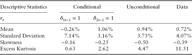
When S = 2, the Markov estimates are μ1 = −0.716 percent, σ1 = 8.018 percent, μ2 = 1.111 percent, and σ2 = 2.906 percent. The transition probability matrix, T, has diagonal elements π11 = 75.04 percent, π22 = 97.44 percent. These six values are all that is required to determine a wide range of model-based summary statistics for asset returns. In Table 4.1, we report both the conditional and unconditional values of the mean, standard deviation, skewness, and excess kurtosis of the return to the market one period ahead and compare these to the equivalent descriptive statistics for the raw data.
From this it is clear that both time-varying expected returns and heteroskedasticity are introduced by allowing for asset returns to be described by a mixed normal distribution through a Markov regime switching process. The unconditional data also contain clear excess kurtosis. State 1 is a bear state with negative expected returns and high volatility, while State 2 has slightly above average returns and lower volatility. The proportion of time that the economy spends in State 1 (State 2) is 9.3 percent (90.7 percent), which is taken directly from S, the left eigenvector of T. The expected length of stay in each state on each visit is given by (1 − πjj)−1, and this is equal to four months in State 1 and over three years in State 2.
At first sight, though, this calibration appears to be inconsistent with market equilibrium. If State 1 can be fully identified at the time it occurs, then all rational risk-averse investors would wish to immediately remove their money from the volatile stock market because of the negative expected returns in this state. This issue is at least in part overcome by the fact that the state variable δjt is not directly observable. Instead, the Markov estimation process produces values pjt, which gives the probability that δjt = 1. The expected return contingent on information available at time t − 1 is given by ![]() , with similar expressions following for higher moments. For example, the Markov estimate for February 2014 is that p1t = 1.4 percent, giving an expected return for March 2014 of 1.05 percent.
, with similar expressions following for higher moments. For example, the Markov estimate for February 2014 is that p1t = 1.4 percent, giving an expected return for March 2014 of 1.05 percent.
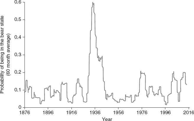
Figure 4.2 presents the average estimate of p1t during the previous 60 months for the total horizon of the available data, 1876–2014.
As we might expect, p1t takes its greatest values at times consistent with market participants’ beliefs about the occurrence of bear markets: the 1930s, 1970s, and 2000s.5 The appeal of Markov switching models becomes clear from this example. The basic framework is very similar to the standard model, with no requirement to move to more complex distributions than the normal. Markov models are therefore simple to explain intuitively to people familiar with the usual assumption of i.i.n.d. logarithmic asset returns. The considerably improved descriptive power comes purely from switching between states, and these have properties that are likely to be well recognized by those familiar with financial markets. The estimated timings of transition also correspond well with our historical understanding of the way in which the economy has moved between bull and bear markets. This combination of a simple extension from the standard model, intuitively appealing states, and high descriptive accuracy lie behind the widespread use of Markov regime switching models in empirical finance.
THREE-STATE ESTIMATION
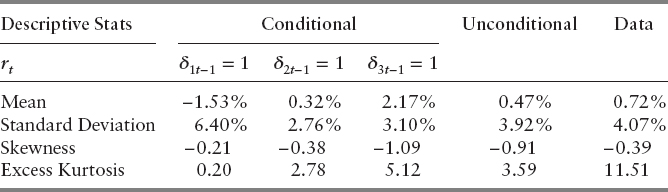
We can further enrich this model by incorporating a further state. Now the conditional and unconditional returns to the market next period are given by Table 4.2.
In principle, we can add more and more states to increase both the complexity of our underlying model and its ability to capture the unconditional moments of the underlying data. However, beyond a certain level, the benefits of parsimony begin to outweigh those of a richer regime setting. Standard model selection metrics, such as the Akaike Information Criterion (AIC), which are standard outputs from Markov estimation software, can be used to determine when there is overfitting from modeling too many states. For the two-, three-, and four-state models, the AIC are 2.754, 2.587, and 2.576, respectively. We should therefore, choose the lowest AIC, so the three-state calibration is preferred to the two-state calibration, and a four-state calibration is mildly preferred to the three-state calibration.
MARKOV MODELS FOR MULTIPLE ASSETS
The extension of this framework to account for the joint time-series properties of multiple assets is straightforward. Denote individual assets by the subscripts a,b, let the expected return and standard deviation of returns to asset a at time t be given by μat, σat respectively, and let the correlation between the returns of asset a and b be given by ρabt. We further use Σt to denote the variance-covariance matrix at this time, with elements ![]() on the diagonal and Σabt = ρabtσatσbt off the diagonal.
on the diagonal and Σabt = ρabtσatσbt off the diagonal.
The usual Markov assumptions now hold, with μat = μaj and Σt = Σj for fixed values of μaj, Σj contingent on the state being j at time t; δjt = 1. This setting not only captures time-varying expected returns and volatility, but also now potentially captures time-variation in cross-sectional correlations.
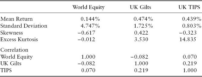
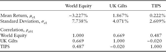
Take as an example the following three asset classes: 10-year UK Treasury bonds (gilts), an index of UK Treasury Inflation-Protected Securities (TIPS), and an index of world equity returns, all denominated in sterling, based on monthly returns for the interval December 1998 to December 2010. The descriptive statistics for these data are shown in Table 4.3.
Surprisingly, over this time period, there is no excess kurtosis in world equity returns as measured in sterling, although the TIPS returns distribution has a very fat tail. The correlation between equities and the other asset classes is also low, but there is some positive correlation between the two classes of fixed income securities.
If we set S = 2, then a Markov model captures this as follows, see Table 4.4.
State 1 is again a very clear bear state with extremely negative expected returns to world equities and with volatilities well above their unconditional values. A particularly notable feature is the high positive correlation in this state between world equities and UK gilts—a characteristic that is completely obscured in the unconditional summary statistics.

State 2 is similar to state 2 in the single-asset example, as it corresponds to a mild bull market for world equities. Now the correlation between world equities and UK gilts is mildly negative. The transition probability matrix has diagonal elements π11 = 86.82 percent, π22 = 99.28 percent. This means that the economy spends approximately 5.2 percent of the time in state 1 and 94.8 percent in state 2 over the long run. The bull market state has an expected duration of almost 12 years, while for the bear market state, it is just over 7 months.6
This can again be further extended to multiple assets, N, and states, S, but the number of parameters that need estimation quickly gets large. There are N(N + 1)/2 values of Σi and N values of μa for each state, plus S(S − 1) value for T, giving a total number of parameters of S(N(N + 3)/2 + S − 1). So, with ten asset classes and four states, there are 272 parameters that require estimation. In nearly all potential applications this will be challenging to estimate robustly, and so, as the number of assets increases, the regime structure must become simpler to allow for effective estimation.
PRACTICAL APPLICATION OF REGIME SWITCHING MODELS FOR INVESTMENT PURPOSES
In these final sections, we explore the practical application of regime switching models for investment purposes—specifically, Markov switching models. A standard Markov switching model assumes two things:
- The modeled world exists in only a finite number, S, of states each one of which is characterized by a suitable multivariate probability distribution (and if relevant other relationships) characterizing the (random) values that variables of interest may take within the model if the world is then in that state. Often, but not always, these distributions will be multivariate normal.
- The probability of shifting from one state to another at the end of each time step is encapsulated in a S × S matrix, the transition matrix with elements πij. Typically, the πij are assumed to be time stationary unless there is strong evidence to the contrary.
INTUITIVE APPEAL OF SUCH MODELS
Markov switching models have several intuitive attractions for financial modeling purposes. These include:
- They can be viewed as natural extensions of ones in which the modeled world is assumed to exist in just one state (the latter being a special case of a Markov switching model with S = 1 and π11 = 1).
- When S > 1 and even if each individual state in the Markov switching model is characterised merely by a multivariate normal distribution, unconditional outcomes typically exhibit heteroskedasticity, excess kurtosis, and other stylized features observed in real-life financial data.
- Most other practical modeling approaches (perhaps all, if the Markovian approach is sufficiently general) can be approximated by Markov switching models, albeit potentially very complicated ones. For example:
- Suppose the world is not actually time varying. We can model this either as a single-state Markovian model with the distributional form applicable to that state being the one we want the world to exhibit or as a multistate Markovian model, each state of which involves, say, a multivariate normal distribution. This is because any multivariate distribution can be reproduced arbitrarily accurately (in a suitable sense) using merely a distributional mixture of suitably chosen multivariate normal distributions; see for example, Kemp (2011). If we adopt the latter approach then we can achieve the desired time stationarity by selecting the Markov transition matrix so that the probability of ending up in a given final state is the same whatever the initial state, by selecting πij so that for any given j it is the same for all i.
- Suppose the world is time varying but in a way that involves an infinite number of possible states. For example, it exhibits generalized autoregressive conditional heteroskedastic (GARCH) AR(1) behavior in which the volatility of some underlying process, σ, is allowed to take a continuum of values and is updated at time t by reference to its value at time t − 1 together with some random innovation occurring between t − 1 and t. We typically discretize time to approximate the reality of continuous time. We can likewise discretize σ, identifying different regimes for different discretized values that σ is now assumed to be capable of taking. In this instance we would probably also impose constraints on how the different states behave relative to each other, e.g., for a typical GARCH model we might constrain the states so that all features other than the underlying volatility are the same in each state. Of course, if we have m > 1 variables autoregressing at the same time, instead of discretising in one dimension we may need to discretise in m dimensions, vastly increasing the complexity of the model if it is specified in the form of a Markov switching model.
- Suppose the world is time varying but in a way that cannot be captured in a standard Markovian way via state transition probabilities between t − 1 and t that depend only on the state of the world at time t − 1. For example, transition probabilities might exhibit longer-term memories, might themselves be time varying, or might depend on the states of the world at times t − 1, …, t − n. However, an nth order difference equation in a scalar yt = f (yt−1, yt−2, …, yt−n) can be rewritten as a first order difference equation in the vector vt = (yt, yt−1, …, yt−n+1)T. We can likewise reexpress more complicated time dynamics by introducing additional “stacked” states characterized by which underlying states the world was in not just at time t − 1 but at one or more earlier times, again with the downside that this can exponentially increase the effective number of states included in the model.
IMPLEMENTATION CHALLENGES
Perhaps the most important practical challenges faced when implementing a Markov switching model for a real-life investor involve:
- Selecting the “right” Markov switching model structure;
- Calibrating the selected model type to suitable data;
- Integrating the Markov switching model selected as per (1) and (2) with a sufficiently realistic model of the assets and liabilities of the investor in question; and
- Drawing the right conclusions from the combined model in (3), if it is being used to make business or investment decisions, given the challenge of identifying robustly the state the world is currently in.
We discuss these challenges next, accepting that there is often overlap between them. As it is not unique to Markov switching models, we have assumed that the outputs of the Markov switching model align with the inputs needed by the investor's asset and liability model.
SELECTING THE “RIGHT” MODEL STRUCTURE
By this, we mean choosing the number of states we wish to consider, the overall structure of each state (e.g., the distributional family used to characterize the state, in contrast to the specific member of that family to be used in practice), the interrelationships (if any) between states that the model is constrained to exhibit, and so on.
The discussion in the section titled “Intuitive Appeal of Such Models” highlights that Markov switching models can approximate essentially any other type of econometric financial model. It also highlights that it is possible to get the same end answers using differently formulated Markov switching models. The flexibility inherent in Markov switching models almost inevitably means that the structure of any eventually selected model will be strongly influenced by the model creator's prior (i.e., expert) views on how the world “ought” to work.
There are, of course, statistical techniques that can to some extent guide such views. For example, we might adopt the principle of parsimony and penalize more complex models over less complex ones using tools such as the Akaike information criterion or the Bayes information criterion (see, e.g., Kemp (2011)). However, the range of possible Markov switching models is so large that, in practice, prior judgment will still play a strong part in framing such models. As always in investment, the key to a successful eventual outcome is a good understanding of the applicable market dynamics.
For the rest of this chapter, we will assume that the model creator has alighted on a sufficiently rich range of plausible model structures (probably based on prior heuristic analysis of applicable data and prior analysis of the economic rationales supporting the selected model structures) to stand a reasonable chance of selecting an appropriate model structure within the confines of his or her computing resources. We then highlight some of the issues that model creators should ideally bear in mind if they wish to select “intelligently” between these plausible model structures and to utilize them effectively for investment purposes. In this context, the range of plausible model structures to be selected from would typically include special cases not otherwise normally associated with Markov switching model approaches, such as a model that incorporates a single (perhaps non-Gaussian) state (which, as noted, is still technically a Markov switching model but with S = 1). This allows the model creator to validate whether it is worth including regime-switching features in the model in the first place, given the added complexities they introduce as also explored next. It should be noted that some of the issues discussed here are generic to model selection rather than being specific to Markov switching models.
CALIBRATING THE SELECTED MODEL TYPE TO SUITABLE DATA
Markov switching models face the same sorts of issues as other model types when it comes to calibrating model parameters, with the added complication that there are often greater numbers of parameters involved with a Markov switching model and/or more complicated constraints imposed on how these parameters can interact.
Perhaps the most fundamental challenge is to identify suitable data to use in the first place. Researchers often reach for past datasets because they are objective and relatively easily accessible. However, this assumes that the past will be a good guide to the future. For some purposes it may be better to calibrate to market-implied current estimates of distributional parameters or even to use forward looking data if applicable. Most forward-looking data (e.g., analysts’ expected future returns or volatilities on different asset categories) involves expert judgment, introducing issues like those noted in the previous section. However, many of the potential applications of Markov switching models in a financial context are inherently forward-looking, especially if we are hoping to take financial decisions based on our model rather than merely attempting to understand what might have happened in the past. For such model uses, introducing some expert judgment is generally desirable, as long as the judgment really is “expert.”
Even if we revert merely to using past data, we still need to ask ourselves whether the data we have available are representative of what might happen in the future. Even if it is, are some time periods within it more representative than others? For risk-management purposes, it is increasingly common to require that the dataset include a minimum proportion of “stressed” times. For example, if we would otherwise use a five-year dataset but conditions have been relatively benign over the whole of that period, then we might overwrite the earlier part of the dataset with data from further back in time deemed to relate to less benign conditions. Even for return-optimization purposes, there may be some parts of the data we think are more applicable now than other parts. Indeed, the inherent rationale for using regime-switching models is the recognition that different parts of the past have different characteristics, depending on the state the world was then in.
Assuming that such issues are adequately addressed, we then need to select parameters characterizing the model that best fit the (past) data. This would typically be done algorithmically (via suitable computer software), using some criterion of best fit, such as maximum likelihood. If the states are all multivariate normal, then one way of doing this is to use a Gaussian Mixture Model (GMM) approach as explained in, e.g., Press et al. (2007). The GMM approach identifies the set of S multivariate normal distributions that best represents the observed distribution of the data points from t = 1 to T. If there are m variables of interest in each state, then each of the T data points is an m-dimensional random variable. Part of the output of the GMM algorithm is the probability pt,k that the observation at time t is from state k where 1 ≤ j ≤ S. With enough observations and by comparing pt−1,j with pt,j, we can derive a suitable transition matrix ![]() between the states that matches the observed likelihoods.
between the states that matches the observed likelihoods.
If at outset we haven't decided how many states to include in our model, then such a fitting might be repeated for several different values of S, potentially including penalties for reduced parsimony such as the information criteria referred to in the previous section. If constraints are applied to interrelationships between individual states (e.g., we might require some means, volatilities, or correlations to be identical in two or more states), then the iteration steps within the basic GMM algorithm would need to be suitably refined and any information criterion scores adjusted accordingly.
Several open access or open source versions of the GMM algorithm are available to researchers who do not otherwise have access to this algorithm using commercial packages. These include the open access web-based MnGaussianMixtureModellingSA (http://www.nematrian.com/F.aspx?f=MnGaussianMixtureModellingSA) function in the Nematrian website's online function library (and corresponding spreadsheets). Although the GMM algorithm is normally associated with underlying Gaussian states, it can, in principle, be modified to target other distributional forms (by modifying the appropriate part of the algorithm that encapsulates the likelihood function for each individual state), but we are not aware at the time of writing of open access or open source variants that include such refinements.
Using computer software to carry out such calibrations hides complexities that ideally need to be borne in mind when applying such models in practice. These complexities include:
- Underlying such algorithms are computerized searches for the maximum value of the function used in the best-fit criterion (e.g., here the likelihood function), and this function will almost always be multidimensional. Multidimensional maximization is generally an inherently hard computational problem, e.g., Press et al. (2007). In particular, if the function in question has more than one local peak, then practical maximization algorithms can converge to a spurious local maximum rather than to the desired global maximum. Typically such algorithms are seeded with initial parameter estimates selected by the user (or preselected by the software). One way of testing whether the algorithm appears to be converging to the desired global maximum is to run the algorithm multiple times starting with different initial parameter estimates and see whether the choice of seed affects algorithm output. Gaussian distributional forms tend to be better behaved (and simpler) than non-Gaussian alternatives in this respect, which tends to favor use of models that involve Gaussian underlying states even if economic theory might otherwise hint at more complicated model structures.
- There is arguably an asymmetry in the way in which such an approach handles the state specification versus how it handles the transition matrix specification. Usually, we will have enough observations to be able to replicate exactly the observed transition probabilities
 , so the maximum likelihood aspect of the problem formulation in practice primarily drives selection of the characterization of the individual states. However, this means that the calibrated model can end up flipping between states relatively quickly. This is implicit in a Markov switching approach in which the transition matrix depends only on the immediately preceding state in which the world was in and also means that model results may be sensitive to choice of time step size. However it does not fully accord with an intuitive interpretation of what we mean by a “state.” For example, when commentators talk about being in bear or bull markets, they usually have in mind a state of the world that is expected to persist for quite a few months even if they might be using monthly data to form their views.
 - There are inherent limitations on how accurately the fine structure of covariance matrices can be estimated from finite-sized time series (see, e.g., Kemp, 2011). These apply to Markov switching models as well as to simpler single-state multivariate normal models. Even when the time series are long enough, the fine structure may still in practice be largely indistinguishable from random behavior, making its selection again an exercise in expert judgment. This issue becomes more important when decision outputs from the model are materially affected by these limitations. Unfortunately, portfolio optimization, a common use for financial models, can fall into this category, particularly if the portfolio is being optimized after one or more important drivers of portfolio behavior (such as overall equity market exposure) has been hedged away; see Kemp (2011).
DRAWING THE RIGHT CONCLUSIONS FROM THE MODEL
The final challenge faced by modelers, or at least faced by those employing them, is interpreting the model output in an appropriate manner.
The extent of this challenge will depend heavily on exactly how the model might be used. For example, we might characterize model use for investment purposes under two broad types:
- Reaching a specific investment decision at a particular point in time (e.g., selecting a specific asset allocation stance with the aim of maximizing reward versus risk).
- Seeking generic understanding of likely future market behavior, such as potential range of outcomes for generic downside risk management purposes.
Perhaps the biggest challenge, if we wish to use a Markov switching model for decision-making purposes as in the first type just described, is to work out how best to identify the state of the world we are in at the point in time we are taking our decision. By design with a Markov switching model, different outcomes (over the short-term future) will have different likelihoods, depending on the current state of the world, so our ideal response at the current time should also vary, depending on which state we think we are currently in. If we can't actually tell which state we are in at any given point in time, then we might as well ditch using a Markov switching model and instead replace it with a single universal state endowed with the weighted average characteristics of the original differentiated states.
Of course, algorithms such as GMM do provide probabilities of being in a given state at any point in time, including the current time; see section titled “Calibrating the selected model type to suitable data.” However, if we plan to use such output then we need to take seriously the second complication referred to in the section on Calibrating the Selected Model Type to Suitable Data. As we noted there, the GMM algorithm output typically results in average times within any given state that are modest multiples of the period length of the data being used to estimate the model. However, if the states are to have economic relevance, then we would not expect their average lifetimes to depend on the periodicity of the underlying data. Better, probably, is to use Markov switching models to identify individual states and then to seek out ways of associating different states with different exogenous variables.
For example, we might be able to characterize one of the states in our model as the “bear” state, and we might find that being in such a state has in the past typically been associated with pessimistic market newsfeeds (or high levels of implied volatility …). We might then infer that if market newsfeeds are currently pessimistic (or implied volatility is high …), then we are currently likely to be in the bear state and react accordingly.
However, there are many possible exogenous variables we might consider in this context, and an ever-present risk of alighting on spurious correlations leading to incorrect decision making. As we have already highlighted, sophisticated modeling techniques such as Markov switching models are most useful when they are accompanied by a good understanding of market dynamics, including dynamics not directly captured by the model itself.
In contrast, the need to be able to identify what state of the world we are in at the current time is arguably not so important for more generic downside risk management purposes. For these sorts of purposes we might in any case start with a mindset that is skeptical of any ability to tell reliably which state we are in at the present time. To work out a value-at-risk (VaR) or other similar risk metric, we might then assume a suitably weighted probabilistic average of opening states or, if we wanted to be more prudent, whichever opening state gave the largest VaR for the relevant time horizon.
Finally, it should be noted that the inclusion of regime-switching elements into asset allocation models considerably complicates the mathematics of the underlying asset allocation problem, especially in relation to selection between risky asset classes. The problem becomes inherently time dependent and hence more sensitive to the utility of the investor in question (and how this might vary through time). This is because the risks and rewards of different strategies change through time and vary, depending on the then-state of the world. Issues such as transaction costs that may be glossed over with simpler time-independent models also take on added importance. This is because the optimal asset allocation can be expected to change through time as the state of the world changes.
REFERENCES
Abouraschi, N., I. Clacher, M. Freeman, D. Hillier, M. Kemp, and Q. Zhang. 2014. Pension plan solvency and extreme market movements: A regime switching approach. European Journal of Finance.
Ang A., and G. Bekaert. 2002. International asset allocation with regime shifts. Review of Financial Studies 15: 1137–1187.
_________. 2002. Regime switches in interest rates. Journal of Business and Economic Statistics 20: 163–182.
_________. 2002. Short rate nonlinearities and regime switches. Journal of Economic Dynamics and Control 26: 1243–1274.
_________. 2004. How do regimes affect asset allocation? Financial Analysts Journal, 60: 86–99.
Ang, A., and A. Timmermann. 2011. Regime changes and financial markets. Netspar Discussion Paper Series, #DP 06/2011–068.
Ang, A., G. Bekaert, and M. Wei. 2008. The term structure of real rates and expected inflation. Journal of Finance 63: 797–849.
Bekaert, G., and R. J. Hodrick. 1993. On biases in the measurement of foreign exchange risk premiums. Journal of International Money and Finance 12: 115–138.
Bekaert, G., R. J. Hodrick, and D. Marshall. 2001. Peso problem explanations for term structure anomalies. Journal of Monetary Economics 48: 241–270.
Black, F. 1990. Equilibrium exchange rate hedging. Journal of Finance 45: 899–908.
Boivin, J. 2006. Has U.S. monetary policy changed? Evidence from drifting coefficients and real-time data. Journal of Money, Credit and Banking 38: 1149–1174.
Bollen, N., S. F. Gray, and R. E. Whaley. 2000. Regime switching in foreign exchange rates: Evidence from currency option prices. Journal of Econometrics 94: 239–276.
Bollerslev, T. 1986. Generalized autoregressive conditional heteroskedasticity. Journal of Econometrics 31: 307–327.
Boyle, P. P., and T. Draviam. 2007. Pricing exotic options under regime switching. Insurance Mathematics and Economics 40: 267–282.
Campbell, J. Y., and L. M. Viceira. 2001. Who should buy long-term bonds? American Economic Review 91: 99–127.
Chaieb, I., and V. Errunza. 2007. International asset pricing under segmentation and PPP deviations. Journal of Financial Economics 86: 543–578.
Chkili, W., and D. K. Nguyen. 2014. Exchange rate movements and stock market returns in a regime-switching environment: Evidence for BRICS countries. Research in International Business and Finance 31: 46–56.
Chkili, W., C. Aloui, O. Masood, and J. Fry. 2011. Stock market volatility and exchange rates in emerging countries: A Markov-state switching approach. Emerging Markets Review 12: 272–292.
Cho, S., and A. Moreno. 2006. A small sample study of the new-Keynesian macro model. Journal of Money, Credit and Banking 38: 1461–1481.
Clarida, R., J. Cali, and M. Gertler. 2000. Monetary policy rules and macroeconomic stability: Evidence and some theory. Quarterly Journal of Economics 115: 147–180.
Dahlquist, M., and S. F. Gray. 2000. Regime-switching and interest rates in the European monetary system. Journal of International Economics 50: 399–419.
Ding, Z. 2012. An implementation of Markov regime switching models with time varying transition probabilities in matlab. Available at SSRN: http://ssrn.com/abstract=2083332
Dumas, B., and B. Solnik. 1995. The world price of foreign exchange risk. Journal of Finance 50: 445–477.
Elliot, R. J., and H. Miao. 2009. VaR and expected shortfall: A non-normal regime-switching framework. Quantitative Finance 9: 747–755.
Elliot, R. J., and T. K. Siu. 2009. On Markov modulated exponential affine bond price formulae. Applied Mathematical Finance 16: 1–15.
Engle, R. F. 1982. Autoregressive conditional heteroscedasticity with estimates of the variance of United Kingdom inflation. Econometrica 50: 987–1008.
Engel, C., and J. Hamilton. 1990. Long swings in the dollar: Are they in the data and do markets know it? American Economic Review 80: 689–713.
Fama, E. F., and K. R. French. 2002. The equity premium. Journal of Finance 57: 637–659.
Freeman, M. C. 2011. The time varying equity premium and the S&P500 in the twentieth century. Journal of Financial Research 34: 179–215.
Froot, K. A., and M. Obstfeld. 1991. Exchange-rate dynamics under stochastic regime shifts. Journal of International Economics 31: 203–229.
Guidolin, M. 2012. Markov switching models in empirical finance. Innocenzo Gasparini Institute for Economic Research, Bocconi University Working Paper Series No. 415.
Guidolin, M., and A. Timmermann. 2008. Size and value anomalies under regime shifts. Journal of Financial Econometrics 6: 1–48.
Hamilton, J. D. 1988. Rational expectations econometric analysis of changes in regime: An investigation of the term structure of interest rates. Journal of Economic Dynamics and Control 12: 385–423.
_________. 1989. A new approach to the economic analysis of nonstationary time series and the business cycle. Econometrica 57: 357–384.
Hamilton, J. D., and R. Susmel. 1994. Autoregressive conditional heteroskedasticity and changes in regime. Journal of Econometrics 64: 307–333.
Heinen, C. L. A., and A. Valdesogo. 2009. Modeling international financial returns with a multivariate regime-switching copula. Journal of Financial Econometrics 7: 437–480.
Henkel, S. J., J. S. Martin, and F. Nardari. 2011. Time-varying short-horizon predictability. Journal of Financial Economics 99: 560–580.
Jorion, P. 1990. The exchange rate exposure of U.S. multinationals. Journal of Business 63: 331–345.
Kanas, A. Forthcoming. Default risk and equity prices in the U.S. banking sector: Regime switching effects of regulatory changes. Journal of International Financial Markets, Institutions and Money.
Kemp, M. H. D. 2011. Extreme Events: Robust Portfolio Construction in the Presence of Fat Tails. Hoboken, NJ: John Wiley and Sons.
Lettau, M., S. C. Ludvigson, and J. A. Wachter. 2008. The declining equity premium: What role does macroeconomic risk play? Review of Financial Studies 21: 1653–1687.
Roll, R. 1992. Industrial structure and the comparative behaviour on international stock market indices. Journal of Finance 47: 3–41.
Schwert, G. 1989. Why does stock market volatility change over time? Journal of Finance 44: 1115–1153.
Sims, C., and T. Zha. 2006. Were there regime switches in U.S. monetary policy? American Economic Review 96: 54–81.
Sola, M., and J. Driffill. 2002. Testing the term structure of interest rates using a stationary vector autoregression with regime switching. Journal of Economic Dynamics and Control 18: 601–628.
Stulz, R. (1981). On effects of barriers to international investment. Journal of Finance 36: 923–934.
Welch, I., and A. Goyal. 2008. A comprehensive look at the empirical performance of equity premium prediction. Review of Financial Studies 21: 1455–1508.
Whitelaw, R. 2000. Stock market risk and return: An equilibrium approach. Review of Financial Studies 13: 521–548.
1Some sources define the transition probability matrix as the transpose of this definition, in which case the columns must sum to one.
2We can also calculate the value of these statistics for rt conditional on δit−1 = 1 in an analogous way by replacing Mk with ![]() in these expressions.
in these expressions.
3Data are taken from Robert Shiller's website (http://www.econ.yale.edu/~shiller/data.htm).
4All of our statistics are monthly as we are using monthly data.
5It is worth noting that this is an ex-post statement and not an ex-ante statement, and so we do not know investor expectations beforehand.
6It is worth noting that the results for the one-state and two-state models are quite different, which highlights the need for a Markov model. If we thought they would be the same, or similar, then this would not be the appropriate econometric framework to undertake the analysis.