CHAPTER 5

Output Analysis and Stress Testing for Risk Constrained Portfolios

Jitka Dupačová Miloš Kopa

Department of Probability and Mathematical Statistics, Faculty of Mathematics and Physics, Charles University, Prague, Czech Republic

INTRODUCTION

The main feature of the investment and financial problems is the necessity to make decisions under uncertainty and over more than one time period. The uncertainties concern the future level of interest rates, yields of stock, exchange rates, prepayments, external cash flows, inflation, future demand, and liabilities, for example. There exist financial theories and various stochastic models describing or explaining these factors, and they represent an important part of procedures used to generate the input for decision models.

To build a decision model, one has to decide first about the purpose or goal; this includes identification of the uncertainties or risks one wants to hedge, of the hard and soft constraints, of the time horizon and its discretization, and so on. The next step is the formulation of the model and generation of the data input. An algorithmic solution concludes the first part of the procedure. The subsequent interpretation and evaluation of results may lead to model changes and, consequently, to a new solution, or it may require a what-if analysis to get information about robustness of the results.

In this paper, we shall focus on static, one-period models. Accordingly, let us consider a common portfolio optimization problem: There are I preselected investment possibilities that result from a preliminary security and portfolio analysis. The composition of portfolio is given by the vector of weights x ∈ ^I with components x_i, i = 1, …, I ∑_ix_i = 1, and it should satisfy several constraints, e.g., x_i ≥ 0 ∀i (no short sales are allowed), or various bounds given by legal or institutional investment policy restrictions, bounds on the total number of assets in the portfolio, and so on. These constraints determine the set X of hard constraints, and they must be satisfied. The outcome of a decision x ∈ X is uncertain. We suppose that it depends on a random factor, say ω ∈ Ω; the common assumption is that the probability distribution P of ω is fully specified. Given a realization of ω the outcome of the investment decision x is the return h(x, ω) or the loss f(x, ω) related with the decision x. However, the realization ω is hardly known at the moment of decision making, hence the goal function should reflect the random factor ω as a whole. The traditional approach is to use the expectations E_Ph(x, ω) or E_Pf(x, ω). The problem to solve would be then

Maximization of expected gains or minimization of expected losses means to get decisions that are optimal in average; possible risks are not reflected. Yet this need not be an acceptable goal. The present tendency is to spell out explicitly the concern for hedging against risks connected with the chosen (not necessarily optimal) decision x ∈ X. However, the concept of risk is hard to define. In practice, risk is frequently connected with the fact that the (random) outcome of a decision is not known precisely, that it may deviate from the expectation, and so on. Intuitively, the “outcome” may be the ex-post observed value of the random objective h(, ω) or f(, ω) for the chosen decision ; hence, a decision-dependent one-dimensional random variable. There are various types of risk, their definitions depend on the context, on decision maker's attitude, and they may possess many different attributes. Anyway, to reflect risk in portfolio optimization models, it is necessary to quantify it.

Risk and Deviation Functions

An explicit quantification of risk appears in finance since 1952 in the works of Markowitz (1952), Roy (1952), and others. Since the mid-nineties of the last century, various functions that describe risk, briefly risk functions or deviation functions, have been introduced and their properties studied—see, for example, Pflug and Römisch (2007), Rockafellar and Uryasev (2002), and Rockafellar, Uryasev, and Zabarankin (2006). Incorporating them into the portfolio optimization model makes the model more adequate but also much harder to solve. Moreover, inclusion of risk functions means to design suitable stress tests, to compare alternative choices of risk functions and of probability distributions by multimodeling, to develop stability and robustness analysis, and so on. Applicability of the existing output analysis techniques (e.g., Dupačová (1999, 2009), Dupačová, Hurt, and Štěpán (2002)), depends on the structure of the model, on the assumptions concerning the probability distribution, on the available data, and on hardware and software facilities.

Both in theoretical considerations and in applications, reasonable properties of risk functions are requested. Similarly, as the risk-neutral expected value criterion, risk functions R should not depend on realization of ω but they depend on decisions and on probability distribution P; the value of a risk function will be denoted R(x, P). Coherence of R (monotonicity, translation invariance, positive homogeneity, and subadditivity (Artzner et al. 1999) is mostly expected. Risk functions value at risk (VaR), which is not coherent in general, and the coherent conditional value at risk (CVaR) are special cases of R. Monotonicity with respect to the pointwise partial ordering and subadditivity are evident requirements. Subadditivity, together with positive homogeneity, imply convexity of the risk function. Hence, duality theory can be used to prove that coherent risk functions R arise as the worst-case expectations for a family of probability measures G on Ω; for a finite set Ω the details can be found in Artzner et al. (1999), and the representation can be extended to a broader class of convex risk functions. In general, convexity of risk functions allows to keep a relatively friendly structure of the problem for computational and theoretical purposes, polyhedral property (CVaR introduced in Rockafellar and Uryasev, 2002), or polyhedral risk functions (Eichhorn and Römisch, 2005). It also allows to rely on linear programming techniques for risk-averse linear scenario-based problems.

In the classical mean-risk notion, a measure of risk expresses a deviation from the expected value. The original Markowitz mean-variance approach Markowitz (1952) was later enriched by alternative deviation functions such as semivariance, mean absolute deviation, or mean absolute semideviation. Recently, Rockafellar, Uryasev, and Zabarankin (2006) introduced general deviation functions D(x, P) that preserve the main properties of standard deviation (nonnegativity, positive homogeneity, subadditivity, and insensitivity to a constant shift). Hence, contrary to the coherent risk functions, deviation functions are not affected by the expected value and can be interpreted as measures of variability. As shown in Rockafellar, Uryasev, and Zabarankin (2006), deviation functions are convex, and they correspond one-to-one with strictly expectation bounded risk functions (i.e., translation invariant, positively homogenous, subadditive risk functions satisfying R(x, P) > −E_Pf(x, ω)) under the relations:

where P_c is the centered distribution derived from P. Using duality theory, one can express deviation functions in terms of risk envelopes. For a given x, each deviation function can be paired with the corresponding risk envelope A. For a coherent deviation function the risk envelope A is nonempty, closed, and convex subset of Q = {A : A(ω) ≥ 0, EA = 1}. Hence, the risk envelope is a set of probability distributions and the dual representation of D(x, P) is

where . The dual expression assesses how much worse the expectation E_Pf(x, ω) can be under considered alternative probability distributions P′. These alternative distributions depend on the probability distribution P unlike the risk envelope A. More details can be found in Rock-afellar, Uryasev, and Zabarankin (2006) or in a recent survey, Krokhmal, Uryasev, and Zabarankin (2011). Deviation functions, which can be evaluated using linear programming techniques (in scenario-based problems), mainly CVaR-type deviation functions, are very popular in empirical applications because of their tractability, even for a large number of scenarios.

Risk-Shaping with CVaR [Rockafellar and Uryasev (2002)] Let f(x, ω) denote a random loss defined on X × Ω, α ∈ (0, 1), the selected confidence level, and F(x, P; v) := P{ω : f(x, ω) ≤ v}, the distribution function of the loss connected with a fixed decision x ∈ X. Value at risk (VaR) was introduced and recommended as a generally applicable risk function to quantify, monitor, and limit financial risks and to identify losses that occur with an acceptably small probability. Several slightly different formal definitions of VaR coincide for continuous probability distributions. We shall use the definition from Rockafellar and Uryasev (2002), which applies to general probability distributions: The value at risk at the confidence level α is defined by

Hence, a random loss greater than VaR_α occurs with probability equal (or less than) 1 − α. This interpretation is well understood in the financial practice.

However, VaR_α does not fully quantify the loss and does not in general satisfy the subadditivity property of coherent risk functions. To settle these problems, new risk functions have been introduced (see, e.g., Krokhmal, Palmquist, and Uryasev (2002)). We shall exploit results of Rockafellar and Uryasev (2002) to discuss one of them, the conditional value at risk.

Conditional value at risk at the confidence level α, CVaR_α, is defined as the mean of the α-tail distribution of f(x, ω):

According to Rockafellar and Uryasev (2002), CVaR_α(x, P) can be evaluated by minimization of the auxiliary function

with respect to v. Function Φ_α(x, v, P) is linear in P and convex in v. If f(x, ω) is convex function of x, Φ_α(x, v, P) is convex jointly in (v, x). It means that CVaR_α(x, P) = min_v Φ_α(x, v, P) is convex in x and concave in P. In addition, CVaR_α(x, P) is continuous with respect to α.

If P is a discrete probability distribution concentrated on ω¹, …, ω^S, with probabilities p_s > 0, s = 1, …, S, and x a fixed element of X, then the optimization problem CVaR_α(x, P) = min_v Φ_α(x, v, P) has the form

and it can be further rewritten as

For the special case f(x, ω) = −ω^Tx, mean-CVaR model is a linear programming problem.

Similarly, CVaR deviation function for a discrete probability distribution can be expressed as follows:

In dual form, CVaR deviation function at level α equals

what corresponds to risk envelope A = {A ∈ Q: A(ω) ≤ 1/(1 − α)}.

Risk-shaping with CVaR handles several probability thresholds α₁, …, α_J and loss tolerances b_j, j = 1, …, J. For a suitable objective function G₀(x, P) the problem is to minimize G₀(x, P) subject to x ∈ X and CVaR_αj (x, P) ≤ b_j, j = 1, …, J.

According to Theorem 16 of Rockafellar and Uryasev (2002), this is equivalent to

that is, to a problem with expectation type constraints.

Expected Utility and Stochastic Dominance

An alternative idea could be to use the expected utility or disutility function as a criterion in portfolio selection problems. Such criterion depends on the choice of investor's utility function; to assume its knowledge is not realistic. In empirical applications, several popular utility functions (power, logarithmic, quadratic, S-type) are often used as an approximation of the unknown investor's utility function. Moreover, following Levy (1992) and references therein, one can compare investments jointly for all considered utility functions using stochastic dominance relations. In this case, we shall work with the common choice:

Having two portfolios x, y, and no assumptions about decision maker's preferences, we say that x dominates y by the first-order stochastic dominance (FSD) if no decision maker prefers portfolio y to x; that is, E_Pu(ω^Tx) ≥ E_Pu(ω^Ty) for all nondecreasing utility functions u. Accepting the common assumption of risk aversion, one limits attention to the set of nondecreasing concave utility functions that generates the second-order stochastic dominance. That is, portfolio x dominates portfolio y by the second-order stochastic dominance (SSD) if E_Pu(ω^Tx) ≥ E_Pu(ω^Ty) for all nondecreasing concave utility functions u.

Let H(x, P; z) denote the cumulative probability distribution function of returns h(x, ω). The twice cumulative probability distribution function of returns of portfolio x in point w is defined as:

Similarly, for p, q ∈ (0, 1], we consider a quantile function of returns h(x, ω):

and the second quantile function (absolute Lorenz curve):

We summarize the necessary and sufficient conditions for the first and the second-order stochastic dominance relations (see, e.g., Ogryczak and Ruszczyński (2002), Dentcheva and Ruszczyński (2003), Post (2003), Kuosmanen (2004), Kopa and Chovanec (2008)):

Portfolio x ∈ X dominates portfolio y ∈ X by the first-order stochastic dominance if and only if:

• H(x, P; z) ≤ H(y, P; z) ∀z ∈ or
• H⁽⁻¹⁾(x, P; p) ≥ H⁽⁻¹⁾(y, P; p) ∀p ∈ (0, 1] or
• VaR_α(x, P) ≤ VaR_α(y, P) ∀α ∈ (0, 1], see (5.2).

Similarly, the second-order stochastic dominance relation holds if and only if

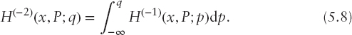
• H⁽²⁾(x, P;w) ≤ H⁽²⁾(y, P; w) ∀w ∈ or
• H⁽⁻²⁾(x, P; q) ≥ H⁽⁻²⁾(y, P; q) ∀q ∈ (0, 1] or
• CVaR_α(x, P) ≤ CVaR_α(y, P) ∀α ∈ [0, 1], see (5.3), or
• E_P[η − ω^Tx]⁺ ≤ E_P[η − ω^Ty]⁺ ∀η ∈ such that both expectations exist, where[.]⁺ = max(0, .).

In general, one can consider any generator of stochastic dominance, especially the choice _N = {u(w) : (−1)ⁿuⁿ(w) ≤ 0 ∀w, n = 1, …, N} gives the Nth-order stochastic dominance relation. Since these relations allow only for pairwise comparisons, one needs to have a benchmark for practical applications of stochastic dominance. Having a benchmark, one can enrich the mean-risk model by stochastic dominance constraints (Dentcheva and Ruszczyński, 2003). Another application of stochastic dominance relations leads to a portfolio efficiency testing whether a given portfolio is the optimal choice for at least one of considered decision makers; see Kopa and Post (2009), Post and Kopa (2013).

Mean-Risk Efficiency

For a chosen risk function, R(x, P) ideas of multiobjective optimization (see, e.g., Ehrgott (2005)) lead to the mean-risk formulations

or

or to inclusion of risk constraints,

or

compare with the mean-variance model of Markowitz (1952) with the random return quantified as h(x, ω) := ω^Tx and risk quantified as the variance or standard deviation of the portfolio yield. See also Krokhmal, Palmquist, and Uryasev (2002) for the risk quantified as the conditional value at risk CVaR, which is known also under the name expected shortfall.

Solutions of any of these problems (for preselected nonnegative parameters λ, a and for k, v such that there exist feasible solutions of (5.11), (5.12)) are mean-risk efficient. At least theoretically, the whole mean-risk efficient frontier can be constructed; see Ruszczyński and Vanderbei (2003) for an application of parametric programming in the case of the Markowitz mean-variance efficient frontier. The previous formulations may be extended to deal with multiple risk functions (see, e.g., Roman, Darby-Dowman, and Mitra (2007)) for “mean-variance-CVaR” model.

Formulations (5.9) or (5.10) with a probability independent set of feasible decisions X are convenient for applications of quantitative stability analysis: Sets of parameter values for which a point x₀ ∈ X is an optimal solution (local stability sets) can be constructed, and on these sets, the optimal value is an explicit function of the parameter in question. We refer to Chapter 5 of Bank et al. (1982) for related theoretical results and to Dupačová (2012) and Dupačová, Hurt, and Štěpán (2002) for an application to stability with respect to the choice of λ in the Markowitz model

of the type (5.9).

On the other hand, risk management regulations ask frequently for satisfaction of risk constraints with a prescribed limit v displayed in (5.12). Moreover, (5.12) is favored in practice: Using optimal solutions x(v) for various values of v, one obtains directly the corresponding points [v, E_Pω^Tx(v)] on the mean-risk efficient frontier. Then, the purpose of the study indicates the formulation to be tackled.

Comment: Numerical tractability of the mean-risk problems depends on the choice of the risk function R, on the assumed probability distribution P, and on the choice of random objectives f(x, ω) or h(x, ω). Programs (5.9) to (5.12) are convex for convex risk functions R(•, P), such as CVaR, see Dupačová (2006), Dupačová and Polívka (2007), and for convex random loss f(•, ω) and concave random return h(•, ω). They are equally suitable when the goal is to get a mean-risk efficient decision and/or properties of such decision.

Robustness and Output Analysis (Stress Testing)

As the probability distribution P is fully known only exceptionally, there is a growing interest in robustness of portfolio optimization problems. Since several large financial disasters in the nineties of the last century, observing various risk functions and stress testing has entered the praxis of financial institutions. We shall focus on output analysis and stress testing with respect to uncertainty or perturbations of input data for static risk portfolio optimization problems, which involve risk considerations.

Moreover, for the sake of numerical tractability, various approximation schemes have been proposed to solve the resulting optimization problems. For example, one may approximate P by a discrete probability distribution based on historical data, by a probability distribution belonging to a given parametric family with an estimated parameter, and so on. The popular sample average approximation (SAA) method solves these problems using a sample counterpart of the optimization problem; that is, instead of P it uses an empirical distribution based on independent samples from P, and asymptotic results can support decisions concerning recommended sample sizes. See Shapiro (2003), Wang and Ahmed (2008), and references therein. The choice of a suitable technique depends on the form of the problem, on the available information and data. Anyway, without additional analysis, it will be dangerous to use the obtained output (the optimal value and the optimal investment decision based on the approximate problem) to replace the sought solution of the “true” problem. Indeed, the optimal or efficient portfolios are rather sensitive to the inputs, and it is more demanding to get applicable results concerning the optimal solutions—optimal investment policies—than robustness results for the optimal value.

Besides focused simulation studies (e.g., Kaut et al. (2007)) and backtesting, there are two main tractable ways for analysis of the output regarding changes or perturbation of P—the worst-case analysis with respect to all probability distributions belonging to an uncertainty set P or quantitative stability analysis with respect to changes of P by stress testing via contamination; see Dupačová (2006, 2009), Dupačová and Polívka (2007), Dupačová and Kopa (2012, 2014). We shall present them in the next two sections.

WORST-CASE ANALYSIS

The worst-case analysis is mostly used in cases when the probability distribution P is not known completely, but it is known to belong to a family P of probability distributions. It can be identified by known values of some moments, by a known support, by qualitative properties such as unimodality or symmetry, by a list of possible probability distributions, or by scenarios proposed by experts with inexact values of probabilities. The decisions follow the minimax decision rule; accordingly, the investor aims at hedging against the worst possible situation.

The “robust” counterpart of (5.9) is

whereas for (5.12) we have

or equivalently, subject to the worst-risk constraint

If R(x, P) is convex in x on X and linear (in the sense that it is both convex and concave) in P on P, then for convex, compact classes P defined by moment conditions and for fixed x, the maxima in (5.13), (5.15) are attained at extremal points of P. It means that the worst-case probability distributions from P are discrete. In general, these discrete distributions depend on x. Under modest assumptions this result holds true also for risk functions R(x, P) that are convex in P. Notice that whereas expected utility or disutility functions and the Expected Regret criterion are linear in P, various popular risk functions are not even convex in P: CVaR(x, P) and variance are concave in P; the mean absolute deviation is neither convex nor concave in P.

Worst-Case Analysis for Markowitz Model (1952)

For the Markowitz model, one deals with the set P of probability distributions characterized by fixed expectations and covariance matrices without distinguishing among distributions belonging to this set. Incomplete knowledge of input data (i.e., of expected returns μ = Eω and covariance matrix V = varω) may be also approached via the worst-case analysis or robust optimization; see Fabozzi, Huang, and Zhou (2010), Pflug and Wozabal (2007), and Zymler, Kuhn, and Rustem (2013). The idea is to hedge against the worst possible input belonging to a prespecified uncertainty or ambiguity set U. We shall denote M, V considered uncertainty sets for parameters μ and V and will assume that U = M × V. This means to solve

or

or

Consider, for example, U described by box constraints 0 ≤ μ_i ≤ μ_i ≤ μ_i, i = 1, …, I, V ≤ V ≤ V componentwise and such that V is positive definite. With X = {x ∈ ^I : x_i ≥ 0 ∀i, ∑_ix_i = 1}, the inner maximum in (5.16) is attained for μ_i = μ_i ∀i and V = V. The robust mean-variance portfolio is the optimal solution of

We refer to Fabozzi, Huang, and Zhou (2010) for a survey of various other choices of uncertainty sets for the Markowitz model.

Comment: For the class of probability distributions P identified by fixed moments μ, V known from Markowitz model and for linear random objective f(x, ω), explicit formulas for the worst-case CVaR and VaR can be derived (e.g., Čerbáková (2006)), and according to Theorem 2.2 of Zymler, Kuhn, and Rustem (2013), portfolio composition x ∈ X satisfies the worst-case VaR constraint ⇔ satisfies the worst-case CVaR constraint.

Worst-Case (Robust) Stochastic Dominance

Applying the worst-case approach to stochastic dominance relation, Dentcheva and Ruszczyński (2010) introduced robust stochastic dominance for the set of considered probability distributions P: A portfolio x robustly dominates portfolio y by SSD if E_Pu(ω^Tx) ≥ E_Pu(ω^Ty) for all concave utility functions and all P ∈ P. Similarly, one can define a robust FSD relation when the expected utility inequality needs to be fulfiled for all utility functions (allowing also nonconcave ones) and for all P ∈ P. The choice of P is very important and typically depends on the application of the robust stochastic dominance relation. The larger set P is, the stronger the relation would be. If the set is too large, then one can hardly find two portfolios being in the robust stochastic dominance relation, and the concept of robust stochastic dominance is useless. Therefore, Dentcheva and Ruszczyński (2010) considered a convexified closed and bounded neighborhood P of a given P₀. Alternatively, one can follow Zymler, Kuhn, and Rustem (2013) and define P as the set of all probability distributions having the same first and second moments as a given distribution P₀. Typically, distribution P₀ is derived from data—for example, as an empirical distribution.

Example: Robust Second-Order Stochastic Dominance Consider I investments and a benchmark as the (I + 1)-st investment. Let the original probability distribution P₀ of all investments (including the benchmark) be a discrete distribution given by S equiprobable scenarios. They can be collected in scenario matrix:

where are the returns along the s-th scenario and r_i = are scenarios for return of the i-th investment. We will use x = (x₁, x₂, …, x_I+1)^T for the vector of portfolio weights and the portfolio possibilities are given by

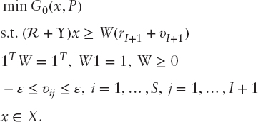
that is, the short sales are not allowed. Then, following Kuosmanen (2004) and Luedtke (2008), the necessary and sufficient condition for the second-order stochastic dominance relation between a portfolio x and the benchmark is: Rx ≥ Wr_I+1 for a double stochastic matrix W (i.e., 1^TW = 1^T, W1 = 1, W ≥ 0 componentwise). Hence the classical optimization problem with SSD constraints (Dentcheva and Ruszczyński (2003)): min G₀(x, P), with respect to all portfolios x that dominate the benchmark by SSD, leads to:

Following Kopa (2010), we consider P containing all discrete probability distributions with S equiprobable scenarios and scenario matrix R_P from the ε-neighbourhood of P₀, that is, satisfying d(P, P₀) ≤ ε. Let matrix be defined as Y = R_P − R and υ_I+1 = (υ_1,I+1, …, υ_S,I+1)^T. Moreover, if d(P, P₀) = max_i,j|υ_ij| then a robust counterpart of (5.19) can be formulated as follows:

STRESS TESTING VIA CONTAMINATION

In practice, approximated or simplified stochastic decision problems are solved instead of the true ones, and it could be misleading, even dangerous, to apply the results without any subsequent analysis such as stress testing, output analysis, or backtesting.

Stress testing is used in financial practice without any generally accepted definition, and it differs among institutions. It appears in the context of quantification of losses or risks that may appear under special, mostly extreme, circumstances. It uses

1. Scenarios that come from historical experience (a crisis observed in the past)—historical stress test, or from the worst-case analysis;
2. Scenarios that might be possible in future, given changes of macroeconomic, socioeconomic, or political factors—prospective stress test, and so on;
3. Recommended, stylized scenarios, such as changes in the interest rates, parallel shift of the yield curve for ±100 bp, changes of the stock index for ±6 percent, of volatility for ±20 percent.

Stress testing approaches differ due to the nature of the tested problem and of the stress scenarios. Performance of the obtained optimal decision is frequently evaluated along these stress, possibly dynamic scenarios, or the model is solved with an alternative input. We shall present stress testing via contamination, which puts together both of these ideas.

Stress testing via contamination was originally derived for the minimization type of model (5.1), with the set X independent of P and for expectation type objective G₀(x, P):= E_Pf(x, ω) to be minimized.

Assume that the problem (5.1) was solved for probability distribution P; denote φ(P) the optimal value and X*(P) the set of optimal solutions. Changes in probability distribution P are modeled using contaminated distributions P_t,

with Q another fixed probability distribution, the alternative or stress distribution. It does not require any specific properties of the probability distribution P. Via contamination, robustness analysis with respect to changes in P gets reduced to much simpler analysis with respect to the scalar parameter t. The objective function in (5.1) is the expectation of the random objective function f(x, ω) (i.e., is linear in P), and we denote it G₀(x, P) to stress its dependence on P. Hence, G₀(x, P_t):= E_Ptf(x, ω) is linear in t and the optimal value function

is concave on [0, 1]. This implies continuity and existence of its directional derivatives on (0, 1). Continuity at t = 0 is property related with stability for the original problem (5.1). In general, one needs that the set of optimal solutions X*(P) is nonempty and bounded.

Stress testing and robustness analysis via contamination with respect to changes in probability distribution P is straightforward for expected disutility models (the objective function is again linear in P). When the risk or deviation measures are concave with respect to probability distribution P, they are concave with respect to parameter t of the contaminated probability distributions P_t, hence, φ(t) is concave and stress testing via contamination can be developed again. The results are contamination bounds for the optimal value function, which quantify the change in the optimal value due to considered perturbations of probability distribution P.

Contamination Bounds

The bounds are a straight consequence of the concavity of the optimal value function φ(t):

For the case of unique optimal solution x*(P) of (5.1) the directional derivative equals G₀(x*(P),Q) − φ(0). In general, each optimal solution x*(P) provides an upper bound

which can be used in (5.20).

Similarly one may construct the upper bound in (5.20) for the optimal value φ(t) on the interval [0, 1] starting from the right end t = 1 of the interval. This provides the right upperbound marked on Figure 5.1.

The obtained contamination bounds (5.20) are global, valid for all t ∈ [0, 1]. They quantify the change in the optimal value due to considered perturbations of (5.1); see the application to stress testing of CVaR by Dupačová and Polívka (2007) and of multiperiod two-stage bond portfolio management problems by Dupačová, Bertocchi, and Moriggia (1998). Notice that to get the bounds (5.20), one has to solve the portfolio problem with the alternative probability distribution Q to get φ(1) and to evaluate the performance G₀(x*(P), Q) of an optimal solution of the original problem in case that Q applies. Both of these calculations appear in various stress tests.

Also, a specific value of contamination parameter t can be fixed in agreement with the stress testing purpose. For stability studies with respect to small changes in the underlying probability distribution, small values of the contamination parameter t are typical. The choice of t may reflect the degree of confidence in expert opinions represented as the contaminating distribution Q, and so on. Using a contaminating distribution Q carried by additional scenarios, one can study the influence of including these additional “out-of-sample” scenarios; also the response on an increasing importance of a scenario can be quantified, and so on.

Example Consider the problem of investment decisions in the international debt and equity markets. Assume that historical data allow us to construct many scenarios of returns of investments in the considered assets categories. We denote these (in principle equiprobable) scenarios by ω^s, s = 1, …, S, and let P be the corresponding discrete probability distribution. Assume that for each of these scenarios, the outcome of a feasible investment strategy x can be evaluated as f(x, ω^s). Maximization of the expected outcome

provides the optimal value φ(P) and an optimal investment strategy x(P).

The historical data definitely do not cover all possible extremal situations on the market. Assume that experts suggest an additional scenario ω*. This is the only atom of the degenerated probability distribution Q, for which the best investment strategy is x(Q)—an optimal solution of max_x∈Xf(x, ω*). The contamination method explained earlier is based on the probability distribution P_t, carried by the scenarios ω^s, s = 1, …, S, with probabilities and by the experts scenario ω* with probability t. The probability t assigns a weight to the view of the expert and the bounds (5.20) are valid for all 0 ≤ t ≤ 1. They clearly indicate how much the weight t, interpreted as the degree of confidence in the investor's view, affects the outcome of the portfolio allocation.

The impact of a modification of every single scenario according to the investor's views on the performance of each asset class can be studied in a similar way. We use the initial probability distribution P contaminated by Q, which is now carried by equiprobable scenarios . The contamination parameter t relates again to the degree of confidence in the expert's view.

Contamination by a distribution Q, which gives the same expectation E_Qω = E_Pω, is helpful in studying resistance with respect to changes of the sample in situations when the expectation of random parameters ω is to be preserved.

Comment The introduced contamination technique extends to objective functions G₀(x, P) convex in x and concave in P including the mean-variance objective function; see Dupačová (1996; 1998; 2006) for the related contamination results. To get these generalizations, it is again necessary to analyze persistence and stability properties of the parametrized problems min_x∈XG₀(x, P_t) and to derive the form of the directional derivative. For a fixed set X of feasible solutions, the optimal value function φ(t) is again concave on [0,1]. Additional assumptions (e.g., Gol'shtein (1970)) are needed to get the existence of its derivative; the generic form is

Contamination Bounds—Constraints Dependent on P

Whereas the stress testing and robustness analysis via contamination with respect to changes in probability distribution P are straightforward when the set X does not depend on P, difficulties appear for models, which contain risk constraints:

subject to

such as the risk shaping with CVaR (5.6). Assume the following:

• X ⊂ ⁿ is a fixed nonempty closed convex set.
• Functions G_j(x, P), j = 0, …, J are convex in x and linear in P.
• P is the probability distribution of the random vector ω with range Ω ⊂ ^m.

Denote X(t) = {x ∈ X: G_j(x, P_t) ≤ 0, j = 1, …, J}, φ(t), X*(t) the set of feasible solutions, the optimal value and the set of optimal solutions of the contaminated problem

The task is again to construct computable lower and upper bounds for φ(t) and to exploit them for robustness analysis. The difficulty is that the optimal value function φ(t) is no more concave in t.

Thanks to the assumed structure of perturbations a lower bound for φ(t) can be derived under relatively modest assumptions. Consider first only one constraint dependent on probability distribution P and an objective G₀ independent of P; that is, the problem is

For probability distribution P contaminated by another fixed probability distribution Q, that is, for P_t:= (1 − t)P + tQ, t ∈ (0, 1) we get

Theorem [Dupačová and Kopa (2012)]

Let G(x, t) be a concave function of t ∈ [0, 1]. Then, the optimal value function φ(t) of (5.24) is quasiconcave in t ∈ [0, 1] and

When also the objective function depends on the probability distribution, that is, on the contamination parameter t, the problem is

For G₀(x, P) linear or concave in P, a lower bound can be obtained by application of the bound (5.25) separately to G₀(x, P) and G₀(x, Q). The resulting bound

is more complicated but still computable.

Multiple constraints (5.21) can be reformulated as G(x, P):= max_jG_j(x, P) ≤ 0, but the function G(x, P) is convex in P. Still for G_j(x, P) = E_Pf_j(x, ω) and for contaminated distributions, G(x, t):= max_jG_j(x, P_t) in (5.24) is a convex piecewise linear function of t. It means that there exists such that G(x, t) is a linear function of t on [0, ] and according to Theorem we get the local lower bound valid for . This bound applies also to objective functions G₀(x, P) concave in P similarly as in (5.27). Notice that no convexity assumption with respect to x was required.

Further assumptions are needed for derivation of an upper bound: Formulas for directional derivative φ′(0⁺) based on Lagrange function L(x, u, t) = G₀(x, P_t) + ∑_ju_jG_j(x, P_t) for the contaminated problem follow, for example, from Theorem 17 of Gol'shtein (1970) if the set of optimal solutions X*(0) and of the corresponding Lagrange multipliers U*(x, 0) for the original, noncontaminated problem are nonempty and bounded. Their generic form is

Nevertheless, to get at least a local upper bound (5.20) means to get X(t) fixed, that is, φ(t) concave, for t small enough. For X convex polyhedral this can be achieved for (5.21) if the optimal solution x*(0) of the noncontaminated problem is a nondegenerated point in which the strict complementarity conditions hold true. Then, for t small enough, t ≤ t₀, t₀ > 0, the optimal value function φ(t) is concave, and its upper bound equals

For a discussion and general references, see Dupačová and Kopa (2012). Differentiability of G_j(•, P_t) can be exploited, but there are rather limited possibilities to construct local upper contamination bounds when neither convexity nor differentiability is present (e.g., for nonconvex problems with VaR constraints). In some special cases, trivial upper bounds are available—for example, if x*(0) is a feasible solution of (5.22) with t = 1, then

See Dupačová and Kopa (2012; 2014).

In the general case, to allow for the stress testing an indirect approach was suggested; see Branda and Dupačová (2012): Apply contamination technique to penalty reformulation of the problem. Then the set of feasible solutions does not depend on P and for approximate problem, global bounds (5.20) follow. See Example 4 of Branda and Dupačová (2012) for numerical results.

Illustrative Examples [Dupačová and Kopa (2012)]

Consider S = 50 equiprobable scenarios of monthly returns of I = 9 assets (8 European stock market indexes: AEX, ATX, FCHI, GDAXI, OSEAX, OMXSPI, SSMI, FTSE, and a risk-free asset) in period June 2004 to August 2008. The scenarios can be collected in the matrix R as in the example titled “Robust second-order stochastic dominance”; however, now without a benchmark, that is, a vector of portfolio weights x = (x₁, x₂, …, x_I)^T is taken from the portfolio possibilities set:

The historical data come from the precrisis period. The data are contaminated by a scenario r^S+1 from September 2008 when all indexes strongly fell down. The additional scenario can be understood as a stress scenario or the worst-case scenario. It can be seen in Table 5.1 presenting basic descriptive statistics of the original data and the additional scenario (A.S.).

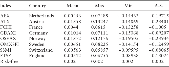
We will apply the contamination bounds to mean-risk models with CVaR as a measure of risk. Two formulations are considered: In the first one, we are searching for a portfolio with minimal CVaR and at least the prescribed expected return. Second, we minimize the expected loss of the portfolio under the condition that CVaR is below a given level.

Minimizing CVaR Mean-CVaR model with CVaR minimization is a special case of the general formulation (5.1) when G₀(x, P) = CVaR(x, P) and G₁(x, P) = E_P(−ω^Tx) − μ(P); μ(P) is the maximal allowable expected loss. We choose

It means that the minimal required expected return is equal to the average return of the equally diversified portfolio. The significance level α = 0.95 and X is a fixed convex polyhedral set representing constraints that do not depend on P. Since P is a discrete distribution with equiprobable scenarios r¹, r², …, r⁵⁰, using (5.5), the mean-CVaR model can be formulated as the following linear program:

By analogy, for the additional scenario we have:

or, equivalently:

where .

First, we compute for t ∈ [0, 1] the optimal value function of the contaminated problem.

where .

Second, applying (5.27), we derive a lower bound for φ(t). Note that now

and

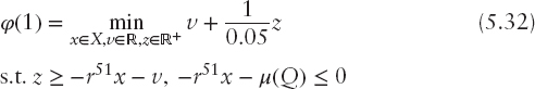
Finally, we construct an upper bound for φ(t). Since the optimal solution x*(0) of (5.31) is a feasible solution of (5.32), we can apply (5.30) as a trivial upper bound for all t ∈ [0, 1]:

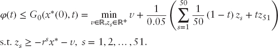
The disadvantage of this trivial bound is the fact that it would require evaluation of the CVaR for x*(0) for each t. Linearity with respect to t does not hold true, but we may apply the upper bound for CVaR derived in Dupačová and Polívka (2007):

This yields an upper estimate for G₀(x*(0), t), which is a convex combination of φ(0) and Φ_α(x*(0), v*(x*(0), P), Q). The optimal value φ(0) is given by (5.31) and

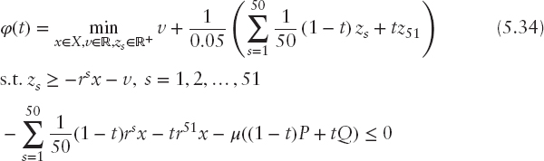
where v* and x* are optimal solutions of (5.31). The graphs of φ(t), its lower bound and two upper bounds (trivial one and its upper estimate) for small contamination t ∈ [0, 0.1] are presented in Figure 5.2. Since all original scenarios have probability 0.02, the performance for t > 0.1 is not of much interest. For t > 0.04, φ(t) in (5.34) coincides with its lower bound because the optimal portfolios consist only of the risk free asset. The upper bound is piecewise linear in t, and for small values of t it coincides with the estimated upper bound.

Minimizing Expected Loss As the second example, consider the mean-CVaR model minimizing the expected loss subject to a constraint on CVaR. This corresponds to (5.21) with G₀(x, P) = E_P(−ω^Tx) and G₁(x, P) = CVaR(x, P) − c where c = 0.19 is the maximal accepted level of CVaR. For simplicity, this level does not depend on the probability distribution. Similar to the previous example, we compute the optimal value φ(t) and its lower and upper bound. Using Theorem 16 of Rockafellar and Uryasev (2002), the minimal CVaR-constrained expected loss is obtained for t ∈ [0, 1] as

and thus equals the optimal value function of the parametric linear program

for t ∈ [0, 1]. In particular, for t = 1 we have

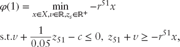
what is equivalent to

compare with (5.33). Using (5.27), we can evaluate the lower bound for φ(t) with

and

Finally, we compute an upper bound for φ(t). Contrary to the previous example, the optimal solution x*(0) of the noncontaminated problem is not a feasible solution of the fully contaminated problem. Therefore, the trivial global upper bound (5.30) cannot be used. We apply instead the local upper bound (5.29) with the directional derivative

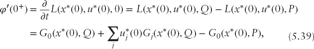
which takes into account the uniqueness of optimal solutions and Lagrange multipliers in (5.28). In this example, the value of multiplier u*(0) corresponding to (5.37) for t = 0 is equal to zero, the CVaR constraint (5.37) is not active, and for sufficiently small t, the upper bound reduces to:

Figure 5.3 depicts the graph of φ(t) given by (5.38) and its lower and upper bound.

The upper bound coincides with φ(t) for t ≤ 0.02. It illustrates the fact that the local upper bound is meaningful if the probability of the additional scenario is not too large—that is, no more than probabilities of the original scenarios for our example.

CONCLUSIONS AND NEW PROBLEMS

Applicability of output analysis techniques depends on the structure of the model, on assumptions concerning the probability distribution, on available data, hardware, and software facilities. Incorporating risk and deviation measures into the portfolio optimization model, presence of stochastic dominance constraints, or presence of multiple stages makes the model much harder to solve. It means to design suitable stress tests, to compare alternative choices of risk measures, utility functions, and of probability distributions by multimodeling, to develop stability and robustness analysis, and so on. Convexity allows keeping a relatively friendly structure of the problem both for computational and theoretical purposes, and polyhedral property allows to rely on linear programming techniques for scenario-based problems with incorporated polyhedral risk measures, such as CVaR. For static models discussed in this chapter, the outcome is a decision dependent one-dimensional random variable; this does not apply to dynamic multistage stochastic decision problems. Modeling suitable multidimensional risk measures and analyzing their properties was initiated by Artzner et al. (2007). It has become an active area of research. Using them in dynamic portfolio optimization brings along various problems connected with model building, scenario generation, and output analysis that have not been solved satisfactorily yet. We refer to Pflug and Römisch (2007), Shapiro, Dentcheva, and Ruszczyński (2009), and numerous references therein.

Acknowledgment: The research was supported by the project of the Czech Science Foundation P402/12/G097, “DYME-Dynamic Models in Economics.”

REFERENCES

Artzner, P., F. Delbaen, J. M. Eber, and D. Heath. 1999. Coherent measures of risk. Mathematical Finance 9: 202–228.

Artzner, P., F. Delbaen, J. M. Eber, D. Heath, and H. Ku. 2007. Coherent multiperiod risk adjusted values and Bellman's principle. Annals of Operations Research 152: 5–22.

Bank, B., J. Guddat, D. Klatte, B. Kummer, and K. Tammer. 1982. Non-Linear Parametric Optimization. Berlin: Akademie-Verlag.

Branda, M., and J. Dupačová. 2012. Approximation and contamination bounds for probabilistic programs. Annals of Operations Research 193: 3–19.

Čerbáková, J. 2006. Worst-case VaR and CVaR. In Operations Research Proceedings 2005 edited by H. D. Haasis, H. Kopfer, and J. Schönberger. Berlin: Springer, 817–822.

Dentcheva D., and A. Ruszczyński. 2003. Optimization with Stochastic Dominance Constraints. SIAM Journal on Optimization 14: 548–566.

Dentcheva D., and A. Ruszczyński. 2010. Robust stochastic dominance and its application to risk-averse optimization. Math. Program. 123: 85–100.

Dupačová, J. 1996. Scenario-based stochastic programs: Resistance with respect to sample. Annals of Operations Research 64: 21–38.

Dupačová, J. 1998. Reflections on robust optimization. In Stochastic Programming Methods and Technical Applications, edited by K. Marti and P. Kall, LNEMS 437. Berlin: Springer, 111–127.

Dupačová, J. 1999. Portfolio optimization via stochastic programming: Methods of output analysis. Math. Meth. Oper. Res. 50: 245–227.

Dupačová, J. 2006. Stress testing via contamination. In Coping with Uncertainty, edited by K. Marti, Y. Ermoliev, and M. Makowski, LNEMS 581. New York: Springer, 29–46.

Dupačová J. 2009. Portfolio Optimization and Risk Management via Stochastic Programming. Osaka University Press.

Dupačová J. 2012. Output analysis and stress testing for mean-variance efficient portfolios. In Proc. of 30th International Conference Mathematical Methods in Economics, edited by J. Ramík and D. Stavárek. Karviná: Silesian University, School of Business Administration, 123–128.

Dupačová, J., M. Bertocchi, and V. Moriggia. 1998. Postoptimality for scenario based financial planning models with an application to bond portfolio management. In Worldwide Asset and Liability Modeling, edited by W. T. Ziemba, and J. M. Mulvey. Cambridge University Press, 263–285.

Dupačová, J., J. Hurt, and J. Štěpán. 2002. Stochastic Modeling in Economics and Finance, Kluwer, Dordrecht.

Dupačová, J., and M. Kopa. 2012. Robustness in stochastic programs with risk constraints. Annals of Operations Research 200: 55–74.

Dupačová, J., and M. Kopa. 2014. Robustness of optimal portfolios under risk and stochastic dominance constraints, European Journal of Operational Research, 234: 434–441

Dupačová, J., and J. Polívka. 2007. Stress testing for VaR and CVaR. Quantitative Finance 7: 411–421.

Ehrgott, M. 2005. Multicriteria Optimization. New York: Springer.

Eichhorn, A., and W. Römisch. 2005. Polyhedral risk measures in stochastic programming. SIAM Journal on Optimization 16: 69–95.

Fabozzi, F. J., D. Huang, and G. Zhou. 2010. Robust portfolios: Contributions from operations research and finance. Annals of Operations Research 176: 191–220.

Gol'shtein, E. G. 1970. Vypukloje Programmirovanije. Elementy Teoriji. Nauka, Moscow. [Theory of Convex Programming, Translations of Mathematical Monographs, 36, American Mathematical Society, Providence RI, 1972].

Kaut, M., H. Vladimirou, S. W. Wallace, and S. A. Zenios. 2007. Stability analysis of portfolio management with conditional value-at-risk. Quantitative Finance 7: 397–400.

Kopa, M. 2010. Measuring of second-order stochastic dominance portfolio efficiency. Kybernetika 46: 488–500.

Kopa, M., and P. Chovanec. 2008. A second-order stochastic dominance portfolio efficiency measure. Kybernetika 44: 243–258.

Kopa, M., and T. Post. 2009. A Portfolio Optimality Test Based on the First-Order Stochastic Dominance Criterion. Journal of Financial and Quantitative Analysis 44: 1103–1124.

Krokhmal, P., J. Palmquist, and S. Uryasev. 2002. Portfolio optimization with conditional-value-at-risk objective and constraints. Journal of Risk 2: 11–27.

Krokhmal, P., S. Uryasev, and M. Zabarankin. 2011. Modeling and Optimization of Risk. Surveys in Operations Research and Management Science 16: 49-66.

Kuosmanen, T. 2004. Efficient diversification according to stochastic dominance criteria. Management Science 50: 1390–1406.

Levy, H. 1992. Stochastic dominance and expected utility: Survey and analysis. Management Science 38: 555–593.

Luedtke, J. 2008. New formulations for optimization under stochastic dominance constraints. SIAM Journal on Optimization 19: 1433–1450.

Markowitz, H. 1952. Portfolio selection. Journal of Finance 6: 77–91.

Ogryczak, W., and A. Ruszczyński. 2002. Dual stochastic dominance and related mean-risk models. SIAM Journal on Optimization 13: 60–78.

Pflug, G. Ch., and W. Römisch. 2007. Modeling, Measuring and Managing Risk. Singapore: World Scientific.

Pflug, G. Ch., and D. Wozabal. 2007. Ambiguity in portfolio selection. Quantitative Finance 7: 435–442.

Post, T. 2003. Empirical tests for stochastic dominance efficiency. Journal of Finance 58: 1905–1932.

Post, T., and M. Kopa. 2013. General Linear Formulations of Stochastic Dominance Criteria. European Journal of Operational Research 230: 321–332.

Rockafellar, R. T., and S. Uryasev. 2002. Conditional value-at-risk for general loss distributions. Journal of Banking and Finance 26: 1443–1471.

Rockafellar, R. T., S. Uryasev, and M. Zabarankin. 2006. Generalized deviations in risk analysis. Finance Stochast. 10: 51–74.

Roman, D., K. Darby-Dowman, and G. Mitra. 2007. Mean-risk models using two risk measures: a multiobjective approach. Quantitative Finance 7: 443–458.

Ruszczyński, A., and A. Shapiro, eds. 2003. Stochastic Programming, Handbooks in OR & MS, Vol. 10. Amsterdam: Elsevier.

Ruszczyński, A., and R. J. Vanderbei. 2003. Frontiers of stochastically nondominated portfolios. Econometrica 71: 1287–1297.

Shapiro, A. 2003. Monte Carlo sampling methods, Ch. 6 in Ruszczyński and Shapiro (2003), pp. 353–425, and Chapter 5 of Shapiro, Dentcheva, and Ruszczyński (2009).

Shapiro, A., D. Dentcheva, and A. Ruszczyński. 2009. Lectures on Stochastic Programming. Philadelphia: SIAM and MPS.

Wang, Wei, and S. Ahmed. 2008. Sample average approximation for expected value constrained stochastic programs. OR Letters 36: 515–519.

Zymler, S., D. Kuhn, and B. Rustem. 2013. Distributionally robust joint chance constraints with second-order moment information. Math. Program. A 137: 167–198.