CHAPTER 10

Stress Testing for Portfolio Credit Risk: Supervisory Expectations and Practices

Michael Jacobs Jr.¹

Pricewaterhouse Cooper Advisory LLP

INTRODUCTION AND MOTIVATION

Modern credit risk modeling (e.g., Merton 1974) increasingly relies on advanced mathematical, statistical, and numerical techniques to measure and manage risk in credit portfolios. This gives rise to model risk (OCC/BOG-FRB 2011) and the possibility of understating inherent dangers stemming from very rare yet plausible occurrences not in our reference data sets. In the wake of the financial crisis (Demirguc-Kunt, Detragiache, and Merrouche 2010; Acharya and Schnabl 2009), international supervisors have recognized the importance of stress testing (ST), especially in the realm of credit risk, as can be seen in the revised Basel framework (Basel Committee on Banking Supervision 2005; 2006; 2009a–e; 2010a; 2010b) and the Federal Reserve's Comprehensive Capital Analysis and Review (CCAR) program. It can be and has been argued that the art and science of stress testing has lagged in the domain of credit, as opposed to other types of risk (e.g., market risk), and our objective is to help fill this vacuum. We aim to present classifications and established techniques that will help practitioners formulate robust credit risk stress tests.

We have approached the topic of ST from the point of view of a typical credit portfolio, such as one managed by a typical medium- or large-sized commercial bank. We take this point of view for two main reasons. First, for financial institutions that are exposed to credit risk, it remains their predominant risk. Second, this significance is accentuated for medium- as opposed to large-sized banks, and new supervisory requirements under the CCAR will now be focusing on the smaller banks that were exempt from the previous exercise. To this end, we will survey the supervisory expectations with respect to ST, discuss in detail the credit risk parameters underlying a quantitative component of ST, develop a typology of ST programs, and finally, present a simple and stylized example of an ST model. The latter “toy” example is meant to illustrate the feasibility of building a model for ST that can be implemented even by less sophisticated banking institutions. The only requirements are the existence of an obligor rating system, associate default rate data, access to macroeconomic drives, and a framework for estimating economic capital. While we use the CreditMetrics² model for estimating economic capital,² we show how this could be accomplished in a simplified framework such as the Basel II IRB model.

Figure 10.1 plots net charge-off rates for the top 50 banks in the United States. This is reproduced from a working paper by Inanoglu, Jacobs, Liu, and Sickles (2013) on the efficiency of the banking system, which concludes that over the last two decades the largest financial institutions with credit portfolios have become not only larger, but also riskier and less efficient. As we can see here, bank losses in the recent financial crisis exceed levels observed in recent history. This illustrates the inherent limitations of backward-looking models and the fact that in robust risk modeling we must anticipate risk, and not merely mimic history.

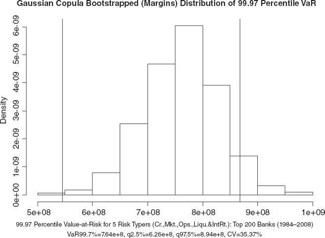
Figure 10.2 shows a plot from Inanoglu and Jacobs (2009), the bootstrap resample (Efron and Tibshirani 1986) distribution of the 99.97th percentile value at risk (VaR) for the top 200 banks in a Gaussian copula model combining five risk types (credit, market, liquidity, operational, and interest rate risk), as proxied for by the supervisory call report data. This shows that sampling variation in VaR inputs leads to huge confidence bounds for risk estimates, with a coefficient of variation of 35.4 percent, illustrating the significant uncertainty introduced as sampling variation in parameter estimates flows through to the risk estimate. This is even assuming we have the correct model!

This chapter shall proceed as follows. The second section discusses conceptual considerations. The following sections cover the function of stress testing; supervisory requirements and expectations; an ST example; and finally, conclusions and discussions of future directions.

CONCEPTUAL ISSUES IN STRESS TESTING: RISK VERSUS UNCERTAINTY

In this section we will consider and survey some of the thoughts regarding the concept of risk. A classical dichotomy exists in the literature, the earliest exposition of which is credited to Knight (1921). He defined uncertainty as the state in which a probability distribution is unknown or cannot be measured. This is contrasted with the situation in which the probability distribution is known or knowable through repeated experimentation. Arguably, in economics and finance (and more broadly in the social or natural as opposed to the physical or mathematical sciences), uncertainty is the more realistic scenario that we are contending with (e.g., a fair vs. loaded die, or a die with an unknown number of sides). We are forced to rely on empirical data to estimate loss distributions, which is complicated by changing economic conditions that invalidate the forecasts our econometric models generate.

Popper (1945) postulated that situations of uncertainty are closely associated with, and inherent with respect to, changes in knowledge and behavior. This is also known as the rebuttal of the historicism concept, that our actions and their outcomes have a predetermined path. He emphasized that the growth of knowledge and freedom implies that we cannot perfectly predict the course of history. For example, a statement that the U.S. currency is inevitably going to depreciate if the United States does not control its debt, is not refutable and therefore not a valid scientific statement, according to Popper.

Shackle (1990) argued that predictions are reliable only for the immediate future. He argues that such predictions affect the decisions of economic agents, and this has an effect on the outcomes under question, changing the validity of the prediction (a feedback effect). This recognition of the role of human behavior in economic theory was a key impetus behind rational expectations and behavioral finance. While it is valuable to estimate loss distributions that help explicate sources of uncertainty, risk managers must be aware of the model limitation that a stress testing regime itself changes behavior (e.g., banks “gaming” the regulators’ CCAR process). The conclusion is that the inherent limitations of this practice is a key factor in supporting the use of stress testing in order to supplement other risk measures. Finally, Artzner and others (1999) postulate some desirable features of a risk measure, collectively known as coherence. They argue that VaR measures often fail to satisfy such properties.

THE FUNCTION OF STRESS TESTING

There are various possible definitions of ST. One common one is the investigation of unexpected loss (UL) under conditions outside our ordinary realm of experience (e.g., extreme events not in our reference data sets). There are numerous reasons for conducting periodic ST, which are largely due to the relationship between UL and measures of risk, examples of the latter being economic capital (EC) or regulatory capital (RC). Key examples of such exercises are compliance with supervisory guidance on model risk management such as the OCC/BOG-FRB (2011) Bulletin 2011–2012 on managing model risk, or bank stress test and capital plan requirements outlined by the Federal Reserve's CCAR program to gauge the resiliency of the banking system to adverse scenarios.

EC is generally thought of as the difference between a value-at-risk measure—an extreme loss at some confidence level (e.g., a high quantile of a loss distribution)—and an expected loss (EL) measure—generally thought of as a likely loss measure over some time horizon (e.g., an allowance for loan losses amount set aside by a bank). Figure 10.3 presents a stylized representation of a loss distribution and the associated EL and VaR measures.

This purpose for ST hinges on our definition of UL. While it is commonly thought that EC should cover EL, it may be the case that UL might not only be unexpected but also not credible, as it is a statistical concept. Therefore, some argue that results of a stress test should be used for EC purposes in lieu of UL. However, this practice is rare, as we usually do not have probability distributions associated with stress events. Nevertheless, ST can be and commonly has been used to challenge the adequacy of RC or EC as an input into the derivation of a buffer for losses exceeding the VaR, especially for new products or portfolios.

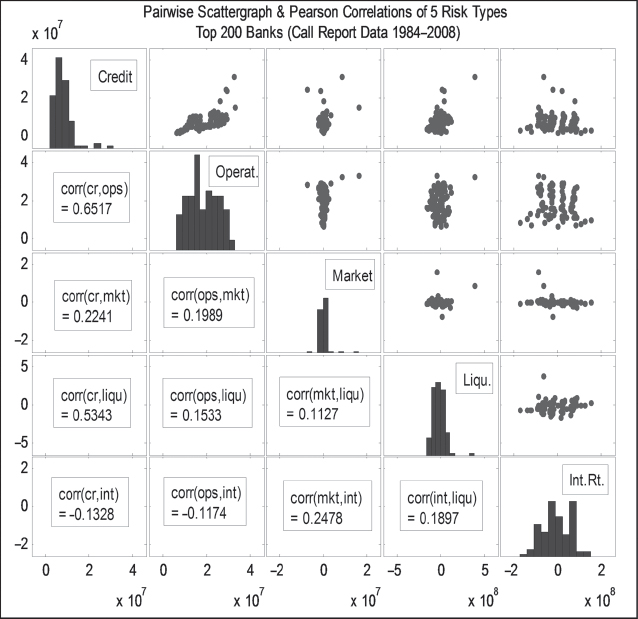
ST has an advantage over EC measures in that it can often better address the risk aggregation problem that arises when correlations among different risk types are in many cases large and cannot be ignored. As risks are modeled very differently, it is challenging to aggregate these into an EC measure. An advantage to ST in determining capital is that it can easily aggregate different risk types (e.g., credit, market, and operational), which is problematic under standard EC methodologies (e.g., different horizons and confidence levels for market vs. credit risk). Figure 10.4 presents the pair-wise correlations for a composite of the top 200 banks for five risk types (credit, market, liquidity, operational, and interest rate risk) as proxies of the call report data. This is evidence of powerful long-run dependencies across risk types. Even more compelling is that such dependencies between risk types are accentuated during periods of stress. See Embrechts, McNeil, and Straumann (2001) and Frey and McNeil (2003) for detailed discussions of correlation and dependency modeling in risk management and various relevant caveats.

A part from risk measurement or quantification, ST can be a risk management tool, used several ways when analyzing portfolio composition and resilience with respect to disturbances. ST can help to identify potential uncertainties and locate the portfolio vulnerabilities such as incurred but not realized losses in value, or weaknesses in structures that have not been tested. ST can also aid in analyzing the effects of new complex structures and credit products for which we may have a limited understanding. ST can also guide discussions on unfavorable developments such as crises and abnormal market conditions, which may be very rare but cannot be excluded from consideration. Finally, ST can be instrumental in monitoring important subportfolios exhibiting large exposures or extreme vulnerability to changes in market conditions.

Quantification of ST appears, and can be deployed, across several aspects of risk management with respect to extreme losses. Primarily, ST can be used to establish or test risk buffers. Furthermore, ST is a tool for helping to determine the risk capacity of a financial institution. Another use of ST is in setting subportfolio limits, especially in low-default situation. ST can also be deployed to inform risk policy, tolerance, and appetite. ST can provide impetus to derive some need for action to reduce the risk of extreme losses and, hence, EC, and it can mitigate the vulnerability to important risk-relevant effects. ST is potentially a means to test portfolio diversification by introducing (implicit) correlations. Finally, ST can help us to question a bank's attitude toward risk.

SUPERVISORY REQUIREMENTS AND EXPECTATIONS

ST appears in the Basel II framework (BCBS 2006), under both Pillar 1 (i.e., minimum capital requirements) and Pillar 2 (i.e., the supervisory review process), with the common aim in both facets of improving risk management. Every bank subject to the advanced internal ratings-based (AIRB) approach to RC has to conduct sound, significant, and meaningful stress testing to assess the capital adequacy in a reasonably conservative way. Furthermore, major credit risk concentrations have to undergo periodic stress tests. It is also the supervisory expectation that ST should be integrated into the internal capital adequacy assessment process (i.e., risk management strategies to respond to the outcome of ST and the internal capital adequacy assessment process).

The bottom line is that banks shall ensure that they dispose of enough capital to meet the regulatory capital requirements even in the case of stress. This requires that banks should be able to identify possible future events and changes in economic conditions with potentially adverse effects on credit exposures and assess their ability to withstand adverse negative credit events.

One means of doing this quantifies the impact on the parameters of probability of default (PD), loss given default (LGD), and exposure at default (EAD), as well as ratings migrations. Special notes on how to implement these requirements—meaning the scenarios that might impact the risk parameters—include the use of scenarios that take into consideration the following:

• Economic or industry downturns
• Market-risk events
• Liquidity shortages
• Recession scenarios (worst case not required)

Banks should use their own data for estimating ratings migrations and integrate the insight of such for external ratings. Banks should also build their stress testing on the study of the impact of smaller deteriorations in the credit environment.

Shocking credit risk parameters can give us an idea of what kind of buffer we may need to add to an EC estimate. Although this type of ST is mainly contained in Pillar 1, it is a fundamental part of Pillar 2, an important way of assessing capital adequacy. To some degree, this explains the nonprescriptiveness for ST in Pillar 2, as the latter recognizes that banks are competent to assess and measure their credit risk appropriately. This also implies that ST should focus on EC as well as RC, as these represent the bank's internal and supervisory views on portfolio credit risk, respectively. ST has been addressed regarding the stability of the financial system by regulators or central banks beyond the Basel II framework in published supplements, including now Basel III (BCBS, 2010a; 2010b).

ST should consider extreme deviations from normal situations that involve unrealistic yet still plausible scenarios (i.e., situations with a low probability of occurrence). ST should also consider joint events that are plausible but may not yet have been observed in reference data sets. Financial institutions should also use ST to become aware of their risk profile and to challenge their business plans, target portfolios, risk politics, and so on.

Figure 10.5 presents a stylized representation of ST for regulatory credit risk, using a version of the Basel IRB formula for stressed PD (see Gordy 2003) through the shocking of the IRB parameters. The solid curve represents the 99.97th percentile regulatory credit capital under the base case of a 1 percent PD, a 40 percent LGD, and credit correlation of 10 percent (ballpark parameters for a typical middle-market exposure or a B+ corporate exposure), which has capital of 6.68 percent of EAD (normalized to unity). Under stressed conditions (PD, LGD, and correlation each increased by 50 percent to 1.5 percent, 60 percent, and 15 percent, respectively), regulatory capital more than doubles to 15.79 percent of EAD.

ST should not only be deployed to address the adequacy of RC or EC, but also be used to determine and question credit limits. ST should not be treated only as an amendment to the VaR evaluations for credit portfolios but as a complementary method, which contrasts with the purely statistical approach of VaR methods by including causally determined considerations for UL. In particular, it can be used to specify extreme losses both qualitatively and quantitatively.

EMPIRICAL METHODOLOGY: A SIMPLE ST EXAMPLE

We present an illustration of one possible approach to ST, which may be feasible in a typical credit portfolio. We calculate the risk of this portfolio in the CreditMetrics model, which has the following inputs:

• Correlation matrix of asset returns
• Ratings transition matrix and PDs
• Credit risk parameters of LGD and EAD
• Term structure of interest rates

In order to implement this methodology, we calculate a correlation matrix from daily logarithmic bond returns. The daily bond indices are sourced from Bank of America Merrill Lynch in the Datastream database from the period 2 January 1997 to 19 December 2011, and include all US-domiciled industrial companies in four ratings classes (Baa-A, Ba, B, and C-CCC). Time series and summary statistics are shown in Figures 10.6 and Table 10.1, respectively. Note that higher-rated bonds actually return and vary more than lower-rated bonds, but the coefficient of variation (CV) is U-shaped. The highest correlations are between adjacent ratings at the high and low ends. Note, also, that some of the correlations are lower and others somewhat higher than the Basel II prescriptions.

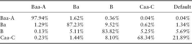
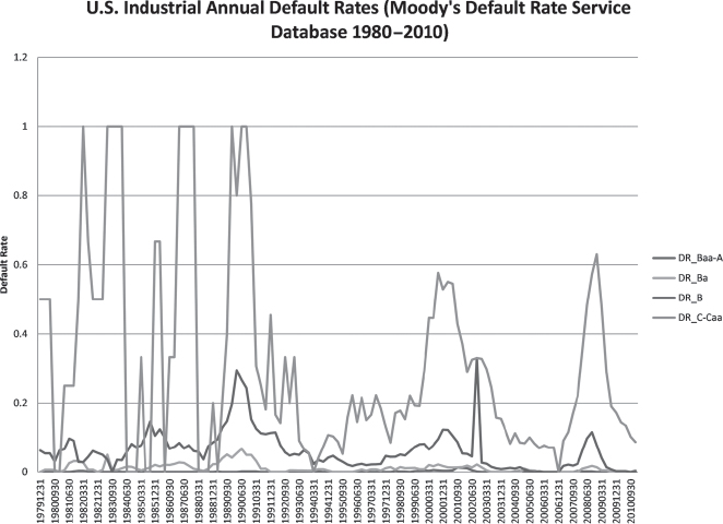
A ratings transition matrix among the rating classes is sourced from Moody's Default Risk Service, shown in Table 10.2. We collapse the best ratings due to paucity of defaults. Note that as ratings worsen, default risks (DRs) increase exponentially, and the diagonals shrink, which is indicative of both higher default risk and greater volatility of ratings for inferior credits. Correlations are also higher between adjacent than separated ratings. Figure 10.7 shows the time series of these default rates, in which the cyclicality of DRs is evident. Table 10.3 shows the summary statistics of the DRs, where we note the high variability relative to the mean of these as ratings worsen.

In order to compute stressed risk, we build regression models for DRs in the ratings classes and stress values of the independent variables to compute stressed PDs. The remainder of the correlation matrix is rescaled so that it is still valid, and this is inputted in the CreditMetrics algorithm.

A search through a large set of variables available from Wharton Research Data Services yielded a set of final explanatory variables that we choose for our model. These variables are all significantly correlated to the Moody's DR and are summarized in Table 10.4. Figure 10.8 shows the VIX measure of volatility or fear in the equity markets and the C&I charge-off rate, the latter being a credit cycle variable found to work well. Figure 10.9 shows the four Fama–French pricing indices (returns on small stocks, value stocks, the broad index, and a momentum strategy), which are also found to be good predictors of DR. Finally, for the factors, Figure 10.10 plots the year-over-year changes in GDP, oil prices, and CPI inflation, which are all macro factors found to be predictive of DRs as well.

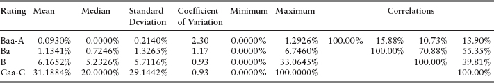
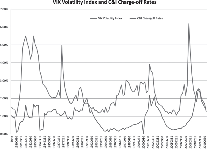
Table 10.5 shows the regression results. All models are highly significant. Estimates are statistically significant across ratings (at least the 5 percent level), and signs on coefficient estimates are all economically sensible.

The regression results shown in Figure 10.11 show that the five Fama–French equity market factors indicate that default rates are lower if broad-market, small, or value stocks are doing better and with higher momentum. Higher market volatility, interest rates, charge-offs, or oil prices increase DRs. DRs are lower if GDP growth or inflation rates are increasing. The magnitude of coefficients varies across ratings, generally greater and more precisely estimated for lower ratings.

Table 10.6 shows the results of the ST for various hypothetical scenarios for our hypothetical portfolio of four bonds. In the base case, expected loss is a normalized 2.63 percent (i.e., EAD is 1), with CreditMetrics EC of 7.17 percent and Basel II IRB RC of 9.29 percent. Note that over most scenarios, RC is bigger, but there are important exceptions; generally, economic scenarios have a bigger stressed EC than RC. In the Uniform ST, the stressing PD/LGD, correlation, and systematic factor shocks have greatest effects. The most severe of the hypothetical scenarios are a spike in market volatility due to a geopolitical disaster, and the “stagflation redux” where we see EC and RC increase by over 100 percent (25 and 30 percent) to 15.27 percent and 17.4 percent (11.9 and 15.3 percent), respectively. We also show the stagflation scenario graphically in Figure 5.6 through plotted loss distributions.

CONCLUSION AND FUTURE DIRECTIONS

We have approached the topic of ST from the point of view of a typical credit portfolio such as one managed by a typical medium- or large-sized commercial bank. We have taken this point of view for two main reasons. First, for financial institutions that are exposed to credit risk, it remains their predominant risk. Second, this importance is accentuated for medium- as opposed to large-sized banks, and new supervisory requirements under the Federal Reserve's CCAR program will now be extended to smaller banks that were exempt from the previous exercise.

To this end, we have surveyed the supervisory expectations with respect to ST, discussed in detail the credit risk parameters underlying a quantitative component of ST, developed a typology of ST programs, and finally, presented a simple and stylized example of an ST model. The latter “toy” example is meant to illustrate the feasibility of building a model for ST that can be implemented even by less sophisticated banking institutions. The only requirements are the existence of an obligor rating system, associate default rate data, access to macroeconomic drives, and a framework for estimating economic capital. While we used the CreditMetrics model for the latter, we showed how this could be accomplished in a simplified framework such as the Basel II IRB model.

There are various fruitful avenues along which we could extend this research program. We could consider alternative risk types in addition to credit, such as market or operational risk, in order to develop a more general framework, which could be applicable to different types of financial institutions (e.g., insurance companies). This would necessarily involve investigating risk aggregation considerations, as discussed by Jacobs and Inanoglu (2009). Second, we could look at this topic from a more international framework, by comparing and contrasting other supervisory frameworks. Third, we could consider frameworks for validating ST modeling frameworks, research analogous to the validation of EC models as addressed by Jacobs (2010). Fourth, we could expand our example of an ST modeling framework to alternative frameworks, such as a top-down approach that models portfolio-level losses and utilizes ARIMA time series techniques. Finally, we could examine the effect of ST on the financial sector as a whole, contributing to the dialogue and debate on the systemic effect of higher capital requirements (Kashyap, Stein, and Hanson 2010).

REFERENCES

Acharya, V. V., and P. Schnabl, 2009, How banks played the leverage game. In Restoring Financial Stability, edited by V. V. Acharya and M. Richardson, Hoboken, NJ: Wiley Finance, pp. 44–78.

Artzner, P., F. Delbaen, J. M. Eber, and D. Heath. 1999. Coherent measures of risk. Mathematical Finance 9 (3): 203–228.

The Basel Committee on Banking Supervision, 2005, July, An explanatory note on the Basel II IRB risk weight functions. Bank for International Settlements, Basel, Switzerland.

_________. 2006, June. International convergence of capital measurement and capital standards: A revised framework. Bank for International Settlements, Basel, Switzerland.

_________. 2009a, May. Principles for sound stress testing practices and supervision, Consultative Paper No. 155. Bank for International Settlements, Basel, Switzerland.

_________. 2009b, July. Guidelines for computing capital for incremental risk in the trading book. Bank for International Settlements, Basel, Switzerland.

_________. 2009c, July. Revisions to the Basel II market risk framework. Bank for International Settlements, Basel, Switzerland.

_________. 2009d, October. Analysis of the trading book quantitative impact study, Consultative Document. Bank for International Settlements, Basel, Switzerland.

_________. 2009e,December. Strengthening the resilience of the banking sector. Consultative Document, Bank for International Settlements, Basel, Switzerland.

_________. 2010a, December. Basel III: A global regulatory framework for more resilient banks and banking systems. Bank for International Settlements, Basel, Switzerland.

_________. 2010b, August. An assessment of the long-term economic impact of stronger capital and liquidity requirements. Bank for International Settlements, Basel, Switzerland.

Demirguc-Kunt, A., E. Detragiache, and O. Merrouche. 2010. Bank capital: Lessons from the financial crisis. International Monetary Fund Working Paper No. WP/10/286.

Efron, B., and R. Tibshirani. 1986. Bootstrap methods for standard errors, confidence intervals, and other measures of statistical accuracy. Statistical Science 1 (1): 54–75.

Embrechts, P., A. McNeil, and D. Straumann. 2001. Correlation and dependency in risk management: Properties and pitfalls. In Risk Management: Value at Risk and Beyond. edited by M. Dempster and H. Moffatt, Cambridge, UK: Cambridge University Press, pp. 87–112,

Frey, R., and A. J. McNeil. 2003. Dependent defaults in models of portfolio credit risk. Journal of Risk 6: 59–62.

Gordy, M. 2003. A risk-factor model foundation for ratings-based bank capital rules. Journal of Financial Intermediation 12 (3): 199–232.

Inanoglu, H., and M. Jacobs Jr., 2009. Models for risk aggregation and sensitivity analysis: An application to bank economic capital. The Journal of Risk and Financial Management 2: 118–189.

Inanoglu, H., M. Jacobs Jr., and A. K. Karagozoglu. 2014, Winter. Bank Capital and New Regulatory Requirements for Risks in Trading Portfolios. The Journal of Fixed Income.

Inanoglu, H., M. Jacobs, Jr., J. Liu, and R. Sickles, 2013 (March), Analyzing bank efficiency: Are “too-big-to-fail” banks efficient?, Working Paper, Rice University, U.S.A.

Jacobs, M. Jr., 2010. Validation of economic capital models: State of the practice, supervisory expectations and results from a bank study. Journal of Risk Management in Financial Institutions 3 (4): 334–365.

Inanoglu, H., and M. Jacobs Jr., 2009. Models for risk aggregation and sensitivity analysis: an application to bank economic capital. Journal of Risk and Financial Management 2: 118–189.

Kashyap, A. K., J. C. Stein, and S. G. Hanson. 2010. An analysis of the impact of “substantially heightened” capital requirements on large financial institutions. Working paper.

Knight, F. H. 1921. Risk, Uncertainty and Profit, Boston, MA: Hart, Schaffner and Marx.

Merton, R. 1974. On the pricing of corporate debt: The risk structure of interest rates, Journal of Finance 29 (2): 449–470.

Moody's Investors Service. 2010. Corporate Default and Recovery Rates, 1920–2010, Special Report, February.

Popper, K. R. 1945. The Open Society and Its Enemies, New York: Routledge and Kegan.

R Development Core Team. 2013. R: A Language and Environment for Statistical Computing, R Foundation for Statistical Computing, Vienna, Austria, ISBN 3–900051–07–0.

Shackle, G. L. S., and J. L. Ford. 1990. “Uncertainty in Economics: Selected Essays,” ed. E.E. Aldershot.

U.S. Office of the Comptroller of the Currency (OCC) and the Board of Governors of the Federal Reserve System (BOG-FRB). 2011. Supervisory Guidance on Model Risk Management (OCC 2011–12), April 4, 2011.