
Chapter 3. Quantifying Output Uncertainty with Monte Carlo Simulation
I of dice possess the science and in numbers thus am skilled.
—King Rituparna of the Mahabharata (circa 900 BCE), on estimating the leaves on a tree from a randomly selected branch
The importance of Monte Carlo simulation (MCS), also known as the Monte Carlo method, cannot be overstated. In finance and investing, MCS is used to value all types of assets, optimize diverse portfolios, estimate risks, and evaluate complex trading strategies. MCS is especially used to solve problems that don’t have an analytical solution.1 Indeed, there are many types of financial derivatives—such as lookback options and Asian options—that cannot be valued using any other technique. While the mathematics underpinning MCS is not simple, applying the method is actually quite easy, especially once you understand the key statistical concepts on which it is based.
MCS also pervades machine learning algorithms in general and probabilistic machine learning in particular. As discussed in Chapter 1 and demonstrated in the simulated solution to the Monte Hall problem in Chapter 2, MCS enables you to quantify the uncertainty of a model’s outputs in a process called forward propagation. It takes the traditional scenario and sensitivity analysis used by financial analysts to a completely different level.
You might be wondering how a method that uses random sampling can lead to a stable solution. Isn’t that a contradiction in terms? In a sense it is. However, when you understand a couple of statistical theorems, you will see that repetition of trials under certain circumstances tames randomness and makes it converge toward a stable solution. This is what we observed in the simulated solution to the Monty Hall problem, where the solution converged on the theoretical values after about 1000 trials. In this chapter, we use MCS to provide a refresher on key statistical concepts and show you how to apply this powerful tool to solve real-world problems in finance and investing. In particular, we apply MCS to a capital budgeting project, in this case a software development project, and estimate the uncertainty in its value and duration.
Monte Carlo Simulation: Proof of Concept
Before we begin going down this path, how do we know that MCS actually works as described? Let’s do a simple proof-of-concept of MCS by computing the value of pi, a known constant. Figure 3-1 shows how we set up the simulation to estimate pi.

Figure 3-1. The blue circle of unit length in a red square with sides of two unit lengths is simulated to estimate the value of pi using MCS
As the Python code shows, you simulate the random spraying of N points to fill up the entire square. Next we count M points in the circle of unit length R. The area of the circle is pi × R2 = M. The length of the square is 2R, so its area is 2R × 2R = 4 × R2 = N. This implies that the ratio of the area of the circle to the area of the square is pi/4 = M/N. So pi = 4 × M/N:
# Import modulesimportnumpyasnpfromnumpyimportrandomasnprimportmatplotlib.pyplotasplt# Number of iterations in the simulationn=100000# Draw random points from a uniform distribution in the X-Y plane to fill#the area of a square that has a side of 2 unitsx=npr.uniform(low=-1,high=1,size=n)y=npr.uniform(low=-1,high=1,size=n)# Points with a distance less than or equal to one unit from the origin will# be inside the area of the unit circle.# Using Pythagoras's theorem c^2 = a^2 + b^2inside=np.sqrt(x**2+y**2)<=1# We generate N random points within our square and count the number of points# that fall within the circle. Summing the points inside the circle is equivalent# to integrating over the area of the circle.# Note that the ratio of the area of the circle to the area of the square is# pi*r^2/(2*r)^2 = pi/4. So if we can calculate the areas of the circle# and the square, we can solve for pipi=4.0*sum(inside)/n# Estimate percentage error using the theoretical value of Pierror=abs((pi-np.pi)/np.pi)*100("After{0}simulations, our estimate of Pi is{1}with an error of{2}%".format(n,pi,round(error,2)))# Points outside the circle are the negation of the boolean array insideoutside=np.invert(inside)# Plot the graphplt.plot(x[inside],y[inside],'b.')plt.plot(x[outside],y[outside],'r.')plt.axis('square');
As in the Monty Hall simulation, you can see from the results of this simulation that the MCS approximation of pi is close to the theoretical value. Moreover, the difference between the estimate and the theoretical value gets closer to 0 as you increase the number of points N sprayed on the square. This makes the ratio of areas of the square and circle more accurate, giving you a better estimate of pi. Let’s now explore the key statistical concepts that enable MCS to harness randomness to solve complex problems with or without analytical solutions.
Key Statistical Concepts
Here are some very important statistical concepts that you need to understand so that you will have deeper insights into why MCS works and how to apply it to solve complex problems in finance and investing. These are also the concepts that provide the theoretical foundation of financial, statistical, and machine learning models in general.
Mean and Variance
Figure 3-2 should refresh your memory of the basic descriptive statistical concepts you learned in high school.
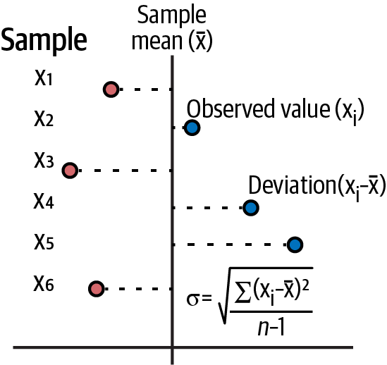
Figure 3-2. Formulas for a sample’s mean and standard deviation2
The arithmetic mean is a measure of the central tendency of a sample of data points. It is simple to calculate: add up all the point values in a sample and divide the sum by the total number of points. Other measures of central tendencies of a dataset are the median and the mode. Recall that the median is the value in the dataset that divides it into an upper and lower half. While the arithmetic mean is sensitive to outliers, the median does not change regardless of how extreme the outliers are. The mode is the most frequent value observed in a data. It is also unaffected by outliers. Sometimes there may be many modes in a sample, and other times a mode may not even exist.
It is important to note that the sum of all deviations from the arithmetic mean of the values always equals zero. That is what makes the arithmetic mean a good measure of the central tendency of a sample. It is also why you have to square the deviations from the mean to make them positive, so they do not cancel one another out. The average deviation from the mean gives you a sense of dispersion, or spread of the data sample, from its arithmetic mean.
Note that the variance of a sample is calculated by adding the sum of the squared deviations and dividing them by one less than the total number of points (n). The reason you use n-1 instead of n is that you have lost a degree of freedom by calculating the mean; i.e. the mean and n-1 points will give you the entire dataset. Standard deviation, which is in the units of the mean, is obtained by taking the square root of variance.
Volatility of asset price returns is calculated using the standard deviation of sample returns. If the returns are compounded continuously in a financial model, such as is assumed in geometric Brownian motion (GBM), we use the natural logarithm of price returns to calculate volatility. This also has the added advantage of making analytical and numerical computations much easier, since the practice of multiplying numbers can be transformed into adding their logarithms. Moreover, when performing multiplications involving numerous values less than 1, the precision of the computation can be compromised due to the inherent numerical underflow limitations of computers.
Expected Value: Probability-Weighted Arithmetic Mean
An important type of arithmetic mean is the expected value of a trade or investment. Expected value is defined as a probability-weighted arithmetic mean of future payoffs:
- E[S] = P(S1) x Payoff(S1) + ....+ P(Sn) x Payoff(Sn)
In finance, you should use expected value to estimate the future returns of your trades and investments. Other measurements used for this purpose are incomplete or misleading. For instance, it is common to hear traders on financial news networks talk about the reward-to-risk ratio of their trades. That ratio is an incomplete metric to consider because it does not factor in the estimated probabilities of positive and negative payoffs. You can structure a trade to have any reward-to-risk ratio you want. It says nothing about how likely you think the payoffs are going to be. If the reward-to-risk ratio is the key metric you’re going to consider in an opportunity, don’t waste your time with investing. Just buy a lottery ticket. The reward-to-risk ratio can go over 100 million to 1.
Why Volatility Is a Nonsensical Measure of Risk
Suppose the price of stock A goes up 5% in one month, 10% the next, and 20% in the third month. The monthly compounded return of A, the geometric mean of the returns, would be about 11.49%, with a monthly standard deviation, or volatility, of 7.64%. Note that we have computed the monthly volatility using the formula in Figure 3-2 and using 2 in the denominator, since this estimate is based on a sample of three months. Compare this to stock B, which declines –10% three months in a row. The monthly compounded return would be –10%, but the monthly volatility would be zero. Which stock would you like in your portfolio?
Volatility is a nonsensical measure of risk because it treats profits that don’t equal the arithmetic mean (a measure of expectation) as risky as losses that do the same. What is also absurd is that losses that meet expectations are not considered a risk. Clearly, a loss is a loss whether or not it equals the average loss of the sample of returns.
Volatility doesn’t consider the direction of the dispersion of returns and treats positive and negative deviations from the mean equally. So, volatility misestimates asymmetric risk. The volatility that investors talk about and don’t want is the semistandard deviation of losses. However, semistandard deviation is analytically intractable and doesn’t lend itself to elegant formulas in financial theories.
This implies that any risk or performance measure that is based on the volatility of returns is inherently flawed. The Sharpe ratio measures asset price returns in excess of a benchmark return and divides that by the volatility of asset price returns. It is a standard investment performance metric popular in academia and industry. However, many value investors, like Warren Buffet, hedge fund managers, and commodity trading advisors reject the Sharpe ratio as a flawed measure of performance. Worse still, volatility underestimates financial risk, which we discuss shortly.
Tip
If your investment’s positive returns are not meeting your expectations and its resultant volatility is keeping you up at night, you may rest assured, as help is nigh. Now you can lower the volatility of your investment returns by transferring those risky, positive return deviations to me for free!
Skewness and Kurtosis
Skewness measures the asymmetry of a distribution about its arithmetic mean. The skewness of a normal distribution is zero. Skewness is computed in a manner similar to that of variance, but instead of squaring the deviation from the mean, you raise it to the third power. This keeps the positive or negative sign of the deviations and so gives you the direction of average deviation from the mean. Skewness tells you where the expected value (mean) of the distribution is with respect to the median and the mode. See Figure 3-3.
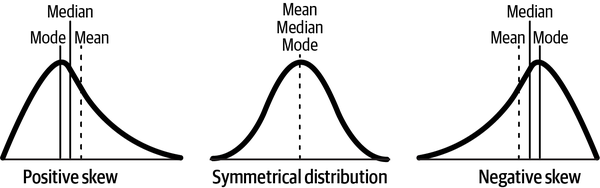
Figure 3-3. Skewed distributions compared to a symmetrical distribution such as the normal distribution3
As an investor or trader, you want your return distribution to be as positively skewed as possible. In a positively skewed distribution, the expected value is going to be greater than the median, and so it will be in the upper half of the distribution—positive returns are going to outweigh the negative returns on average. As discussed earlier, volatility is directionless and so will misestimate asymmetric risks of skewed distributions.
Kurtosis is a measure of how peaked the distribution is about the arithmetic mean and how fat its tails are compared to that of a normal distribution. Like skewness, kurtosis is computed in a manner similar to that of variance, but instead of squaring the deviation from the mean, you raise it to the fourth power. Fat-tailed distributions imply that low probability events are more likely than would be expected if the distribution were normal. A uniform distribution has no tails. In fact, a Cauchy (or Lorentzian) distribution looks deceptively similar to a normal distribution but has very fat tails because of its infinite mean and variance, as shown in Figure 3-4.
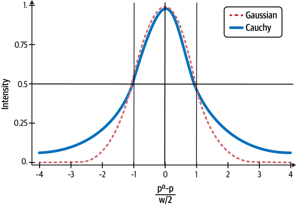
Figure 3-4. Compare the tails of the Cauchy distribution with the normal distribution4
The Gaussian or Normal Distribution
Gaussian distributions are found everywhere in nature and are used in all the sciences. It is quite common to see data distributed like a bell curve, as shown in Figure 3-5. That is why the Gaussian distribution is also called the normal distribution.
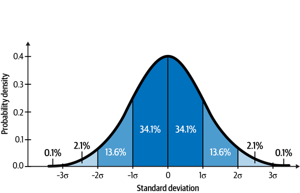
Figure 3-5. About 99.7% of the area of a Gaussian or normal distribution falls within 3 standard deviations from the mean5
Unfortunately, financial data and academic research show that normal distributions are not so common in all financial markets. But that hasn’t stopped most academics and many practitioners from using them for their models. Why? Because Gaussian distributions are analytically tractable and lend themselves to elegant formulas that are solvable without using computers. If you know the mean and standard deviation of a Gaussian distribution, you know everything about the distribution. For instance, in Figure 3-3, you can see that about 68% of the data are within one standard deviation of the mean, 95% are within two standard deviations of the mean, and almost all the data are within three standard deviations of the mean.
Why Volatility Underestimates Financial Risk
The S&P 500 is a global market index and is used by market participants worldwide as a benchmark for the equity market. The index represents an equity portfolio composed of 500 of some of the best companies in the world at any time. Financial instruments based on the S&P 500 are the most liquid markets in the world and operate 24 hours a day for over 5 days of the week. I can attest to that, as I trade the ETF (exchange-traded fund) as well as options and futures based on this index.
According to modern portfolio theory (MPT), asset price returns of the S&P 500 index should be approximately normally distributed. It also assumes that the mean and variance of this distribution are stationary ergodic. What this means is that these two parameters are time invariant, and we can estimate them from a reasonably large sample taken from any time period.
In the following Python code, we test the fundamental tenet of MPT that asset price returns are normally distributed. We import 30 years of S&P 500 price data and compute its daily returns, skewness, and kurtosis:
# Import Python librariesimportpandasaspdfromdatetimeimportdatetimeimportnumpyasnpimportmatplotlib.pyplotaspltplt.style.use('seaborn')# Install web scraper for Yahoo Finance!pipinstallyfinanceimportyfinanceasyf# Import over 30 years of S&P 500 ('SPY') price data into a dataframe# called equitystart=datetime(1993,2,1)end=datetime(2022,10,15)equity=yf.Ticker('SPY').history(start=start,end=end)# Use SPY's closing prices to compute its daily returns.# Remove NaNs from your dataframe.equity['Returns']=equity['Close'].pct_change(1)*100equity=equity.dropna()# Visualize and summarize SPY's daily price returns.# Compute its skewness and kurtosis.plt.hist(equity['Returns']),plt.title('Distribution of S&P 500 Daily PercentageReturnsOverthePast30Years'), plt.xlabel('DailyPercentageReturns'),plt.ylabel('Frequency'),plt.show();("Descriptive statistics of S&P 500 percentage returns:{}".format(equity['Returns'].describe().round(2)))('The skewness of S&P 500 returns is:{0:.2f}and the kurtosis is:{1:.2f}.'.format(equity['Returns'].skew(),equity['Returns'].kurtosis()))
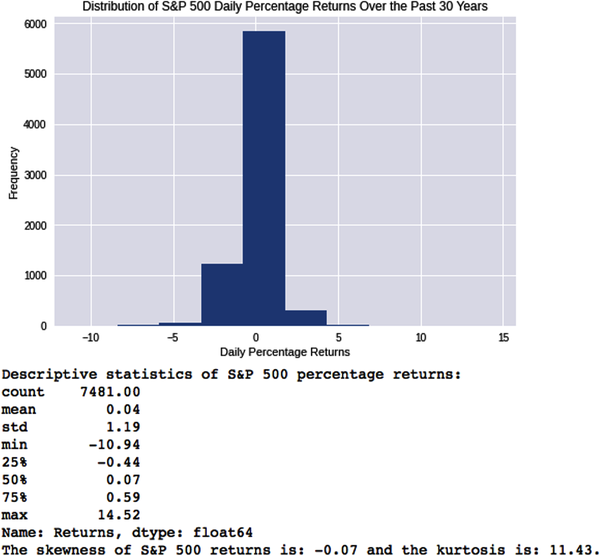
Clearly, the daily return distribution doesn’t look anything close to normal. It has a negative skew of 0.07 and very fat tails with a kurtosis of 11.43. If S&P 500 daily returns were normally distributed, what would it look like? Let’s simulate the world that theoretical finance claims we should be living in.
The time-invariant tenet of MPT implies that we can estimate its statistical moments using a sufficiently large sample from any time period. Thirty years’ worth of data certainly qualifies. We use the mean and standard deviation from the previously mentioned historical data as our estimates for those parameters:
# Estimate the mean and standard deviation from SPY's 30 year historical datamean=equity['Returns'].mean()vol=equity['Returns'].std()sample=equity['Returns'].count()# Use NumPy's random number generator to sample from a normal distribution# with the above estimates of its mean and standard deviation# Create a new column called 'Simulated' and generate the same number of# random samples from NumPy's normal distribution as the actual data sample# you've imported above for SPYequity['Simulated']=np.random.normal(mean,vol,sample)# Visualize and summarize SPY's simulated daily price returns.plt.hist(equity['Simulated']),plt.title('Distribution of S&P 500 SimulatedDailyReturns'), plt.xlabel('SimulatedDailyPercentageReturns'),plt.ylabel('Frequency'),plt.show();("Descriptive statistics of S&P 500 stock's simulated percentagereturns:n{}".format(equity['Simulated'].describe()))# Compute the skewness and kurtosis of the simulated daily price returns.('The skewness of S&P 500 simulated returns is:{0}andthekurtosisis:{1}.'.format(equity['Simulated'].skew().round(2), equity['Simulated'].kurtosis().round(2)))
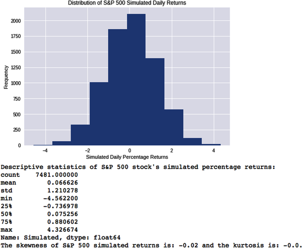
Since we are sampling randomly from a normal distribution, the values for both skewness and kurtosis have minor sampling errors around zero. Regardless, the two distributions look nothing like each other. The daily returns of the S&P 500 over the last 30 years are certainly not normally distributed.
Most financial time series are asymmetric and fat-tailed. These are not nice-to-know financial and statistical trivia. Asset price return distributions with negatively skewed, fat tails have the potential to bankrupt investors, corporations, and entire economies if their modelers ignore them, since they would be underestimating the probabilities of extreme events. The Great Financial Crisis is a recent reminder of the devastating consequences of building theoretical models using elegant mathematical equations that ignore the basic principles of the scientific method and the noisy, ugly, fat-tailed realities of real-world data.
The Law of Large Numbers
This is one of the most important statistical theorems. The law of large numbers (LLN) says that if samples are independent and drawn from the same distribution, the sample mean will almost surely converge to the theoretical mean as the sample size grows larger. In Figure 3-6, the value of the sum of all the numbers that appear on each throw of a die divided by the total number of throws or trials approaches 3.5 as the number of trials increases.
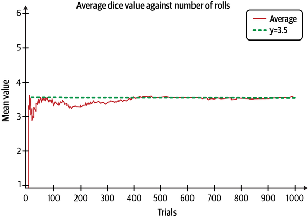
Figure 3-6. The sample mean of dice throws approaches its theoretical mean as the sample size gets larger6
Note that the theoretical average does not have to be a physical outcome. There is no 3.5 on any fair die. Also, notice how the outcomes of the first few trials vary widely about the mean. However, in the long run, they converge inexorably to the theoretical mean. Of course, we assume that the die is fair and that we don’t know the physics of the dice throws.
The Central Limit Theorem
The central limit theorem (CLT) says that if you keep taking samples from an unknown population of any shape and calculate the mean of each of the samples of size n, the distribution of these sample means will be normally distributed, as shown in Figure 3-7.
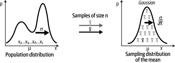
Figure 3-7. The sampling distribution of the sample mean is normally distributed7
This is one of the most amazing statistical phenomena. To appreciate the power of the CLT, consider a fair die that has a uniform distribution since each number on the die is equally likely at ⅙. Figure 3-8 shows what happens when you roll a fair die and add the numbers that show up on each throw and repeat the trials many times. Behold the magic of the CLT: horizontal lines are transformed into an approximate bell curve. If we increase the number of trials or tosses of the die, the curve will look like a bell curve.
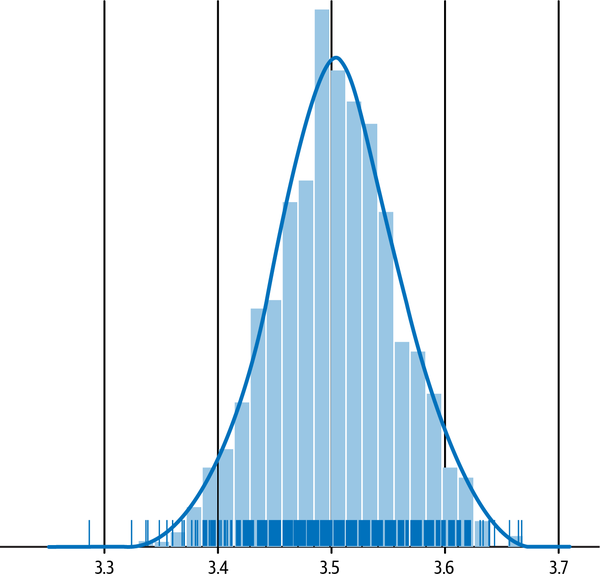
Figure 3-8. The CLT shows us how the uniform distribution of a fair die is transformed into an approximate Gaussian distribution8
Theoretical Underpinnings of MCS
MCS is based on the two most important theorems in statistics already mentioned: the law of large numbers (LLN) and the central limit theorem (CLT).9 Recall that the LLN ensures that as the number of trials increases, the sample mean almost surely converges to the theoretical or population mean. The CLT ensures that the sampling errors or fluctuations of the sample averages from the theoretical mean become normally distributed as sample sizes get larger.
One of the reasons MCS works and is scalable to multidimensional problems is that the sampling error is independent of the dimension of the variable. This sampling error approaches zero asymptotically as the square root of the sample size and not the dimension of the variable. This is very important. It implies that a sampling error in an MCS is the same for a single variable as it is for a 100-dimensional variable.
However, the error decreases as the square root of the sample size n. So you have to increase the MCS iterations by a factor of 100 to increase the accuracy of its estimate by a single digit. But with computing power becoming cheaper by the day, this is not as big an issue now as it was in the last century.
Valuing a Software Project
Let’s increase our understanding of MCS by applying it to a real-life financial problem such as valuing a capital project. The discounted cash flow (DCF) model discussed in the previous chapter is used extensively in corporations worldwide for valuing capital projects and other investments like bonds and equities. A discounted cash flow (DCF) model forecasts expected free cash flows (FCF) over N periods, typically measured in years. FCF in a time period equals cash from operations minus capital expenditures. The model also needs an estimate of the rate of return (R) per period required by the firm’s investors. This rate is called the discount rate because it is used to discount each of the N period FCFs of the project to the present. The reason the FCFs are discounted is that we need to account for an investor’s opportunity cost of capital for undertaking the project instead of another investment of similar risk. The model is set up in four steps:
Forecast the expected free cash flows (FCFs) of the project for each of the N periods.
Estimate the appropriate opportunity cost or discount rate (R) per period.
Discount each period’s expected FCFs back to the present.
Add the discounted expected FCFs (previously described) to get the expected net present value (NPV):
- Expected NPV of project = FCF0 + FCF1 / (1 + R) + FCF2 / (1 + R)2 + ...+ FCFn / (1 + R)N
The NPV decision rule says that you should accept any investment whose expected NPV is greater than zero. This is because an investment with a positive expected NPV gives investors a higher rate of return than an alternative investment of similar risk, which is their opportunity cost.
To create our DCF model, we need to focus on the main drivers of costs and revenues for our software project. We also need to make sure that these variables are not strongly correlated with one another. Ideally, all FCFs of the model should be formulated using very few noncorrelated variables or risk factors.
As you know, software development is labor intensive, and so our main cost driver will be salaries and wages. Also, some developers will be working part time and some full time on the project. However, for developing the cost of labor, we only need the full-time equivalent (FTE) of the effort involved in producing the software, i.e., we estimate the effort as if all required developers were working full time. Scheduling is where we will figure out how much time to allot and when we will need each developer:
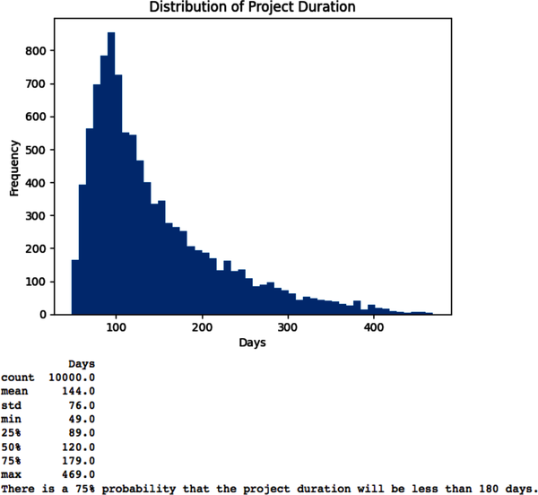
# Import key Python libraries and packages that we need to process and analyze# our dataimportpandasaspdfromdatetimeimportdatetimeimportnumpyasnpfromnumpyimportrandomasnprimportmatplotlib.pyplotaspltplt.style.use('seaborn')# Specify model constants per full-time equivalent (fte)daily_rate=400technology_charges=500overhead_charges=200# Specify other constantstax_rate=0.15# Specify model risk factors that have little or no correlation among them.# Number of trials/simulationsn=10000# Number of full-time equivalent persons on the teamfte=npr.uniform(low=1,high=5,size=n)# In person days and driven independently by the scope of the projecteffort=npr.uniform(low=240,high=480,size=n)# Based on market research or expert judgment or bothprice=npr.uniform(low=100,high=200,size=n)# Independent of price in the price range consideredunits=npr.normal(loc=1000,scale=500,size=n)# Discount rate for the project period based on risk of similar effortsdiscount_rate=npr.uniform(low=0.06,high=0.10,size=n)# Specify how risk factors affect the project modellabor_costs=effort*daily_ratetechnology_costs=fte*technology_chargesoverhead_costs=fte*overhead_chargesrevenues=price*units# Duration determines the number of days the project will take to complete# assuming no interruption. Different from the elapsed time of the project.duration=effort/fte# Specify target_valuefree_cash_flow=(revenues-labor_costs-technology_costs-overhead_costs)*(1-tax_rate)# Simulate project NPV assuming initial FCF=0npv=free_cash_flow/(1+discount_rate)# Convert numpy array to pandas DataFrame for easier analysisNPV=pd.DataFrame(npv,columns=['NPV'])# Estimate project duration in daysDuration=pd.DataFrame(duration,columns=['Days'])# Plot histogram of NPV distributionplt.hist(NPV['NPV'],bins=50),plt.title('Distribution of Project NPV'),plt.xlabel('Project NPV'),plt.ylabel('Frequency'),plt.show();(NPV.describe().round())success_probability=sum(NPV['NPV']>0)/n*100('There is a{0}% probability that the project will have a positive NPV.'.format(round(success_probability)))# Plot histogram of project duration distributionplt.hist(Duration['Days'],bins=50),plt.title('Distribution of Project Duration'),plt.xlabel('Days'),plt.ylabel('Frequency'),plt.show();(Duration.describe().round())
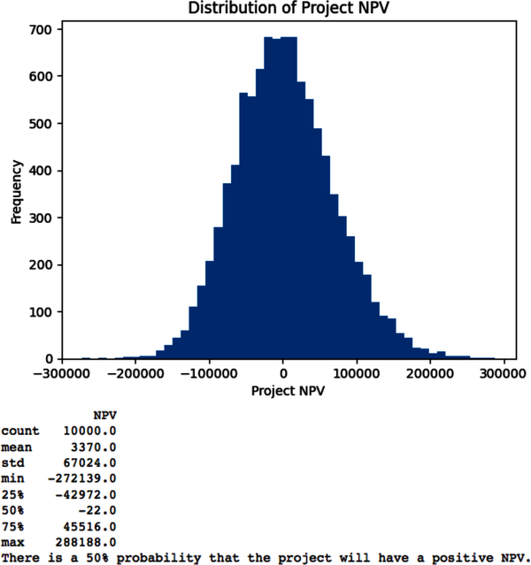
Note that we did not discount the FCF distributions at the risk-free rate. The risk-free rate is the interest rate on a government security such as the US 10-year note. This is a common mistake in NPV simulations, but is incorrect, since each simulation is estimating the expected value of the FCF. Each FCF needs to be discounted at the risk-adjusted discount rate to account for the total risk of the project.
The distribution of risk-adjusted NPVs in the code output needs to be interpreted with caution. Using the dispersion of NPVs to make decisions would double count project risk. Using dispersion of NPVs adjusted at the risk-free rate to account for total risk has no sound theoretical basis in corporate finance.
Building a Sound MCS
To harness the power of MCS to solve complex financial and investment-related problems in the face of uncertainty, it is important that you follow a sound and replicable process. Here is a 10-step process for doing just that:
Formulate how target/dependent variables of your model are affected by features/independent variables, also called risk factors in finance.
Specify the probability distribution of each risk factor. Some common ones include Gaussian, Student’s t-distribution, Cauchy, and binomial probability distributions.
Specify initial values and how time is discretized, such as in seconds, minutes, days, weeks, or years.
Specify how each risk factor changes over time, if at all.
Specify how each risk factor is affected by other risk factors. This is important since correlation among risk factors can incorrectly amplify or dampen effects. This phenomenon is also called multicollinearity.
Let the computer draw a random value from the probability distribution of each independent risk factor.
Compute the value of each risk factor based on that random value.
Compute target/dependent variables based on the computed value of all risk factors.
Iterate steps 6–8 as many times as necessary.
Record and analyze descriptive statistics of all iterations.
The power of MCS is that it transforms a complex, intractable problem that involves integral calculus into a simple one of descriptive statistics with its sampling algorithms. However, there are many challenges to building a sound MCS. Here are the most important ones:
Specifying how each independent variable changes over time. Serial correlation (also known as autocorrelation) is the correlation of a variable with an instance of itself in the past. This correlation is not constant and usually changes over time, especially in financial markets.
Specifying how each feature/independent variable is affected by other independent variables of the model. Correlations among independent variables/risk factors usually change over time.
Fitting a theoretical probability distribution to the actual outcomes. Probability distributions of variables usually change over time.
Convergence to the best estimate is nonlinear, making it slow and costly. It may not occur quickly enough to be of any practical value to trading or investing.
These challenges can be met as follows:
Rigorous data analysis, domain knowledge, and industry expertise. You need to balance rigorous financial modeling with time, cost, and the effectiveness of the models that you produce.
Treat all financial models as flawed and imperfect guides. Don’t let the mathematical jargon intimidate or lull you into a false sense of security. Remember the adage “All models are wrong, but some are useful.”
Managing risk is of paramount importance. Always size capital positions appropriately, have wide error margins, and fallback plans if models fail.
Clearly, there is no substitute for managerial experience and business judgment. Rely on your common sense, be skeptical, and ask difficult questions of a model’s assumptions, inputs, and outputs.
Summary
Fundamentally, MCS is a set of numerical techniques that uses random sampling of probability distributions for computing approximate estimates or for simulating uncertainties of outcomes of a model. The central idea is to harness the statistical properties of randomness to develop approximate solutions to complex deterministic models and analytically intractable problems. MCS transforms a complex, often intractable, multidimensional problem in integral calculus into a much easier problem of descriptive statistics that any practitioner can use.
MCS is especially useful when there is no analytically tractable solution to a problem you are trying to solve. It enables you to quantify the probability and impact of all possible outcomes given your assumptions. It should be used when the traditional analysis of best-, worst-, and base-case scenarios may be inadequate for your decision making and risk management. MCS gives you a better understanding of the risk of complex financial models. Monte Carlo methods are one of the most powerful numerical tools and are pivotal to probabilistic machine learning.
In this chapter, we have applied MCS using independent random sampling. This involves randomly selecting samples from a probability distribution, with each sample being independent of any previous samples. This approach is efficient for simulating simple target probability distributions when samples are not correlated.
However, when dealing with complex target distributions and correlated samples, we have to use more advanced correlated random sampling methods. These dependent random sampling Monte Carlos are crucial to probabilistic machine learning. In Chapter 6, we will examine Markov chain Monte Carlo (MCMC) methods, which are powerful techniques for sampling from complex distributions with dependencies. In Chapter 7, we will apply these methods to financial modeling using the PMC library.
References
Brandimarte, Paolo. Handbook in Monte Carlo Simulation: Applications in Financial Engineering, Risk Management, and Economics. Hoboken, NJ: John Wiley & Sons, 2014.
Cemgil, A. Taylan. “A Tutorial Introduction to Monte Carlo Methods, Markov Chain Monte Carlo and Particle Filtering.” In Academic Press Library in Signal Processing: Volume 1: Signal Processing Theory and Machine Learning, edited by Paulo S. R. Diniz, Johan A. K. Suykens, Rama Chellappa, and Sergios Theodoridis, 1065–1114. Oxford, UK: Elsevier, 2014.
1 Paolo Brandimarte, “Introduction to Monte Carlo Methods,” in Handbook in Monte Carlo Simulation: Applications in Financial Engineering, Risk Management, and Economics (Hoboken, NJ: John Wiley & Sons, 2014).
2 Adapted from an image on Wikimedia Commons.
3 Adapted from an image on Wikimedia Commons.
4 Adapted from an image on Wikimedia Commons.
5 Adapted from an image on Wikimedia Commons.
6 Adapted from an image on Wikimedia Commons.
7 Adapted from an image on Wikimedia Commons.
8 Adapted from an image on Wikimedia Commons.
9 A. Taylan Cemgil, “A Tutorial Introduction to Monte Carlo Methods, Markov Chain Monte Carlo and Particle Filtering,” in Academic Press Library in Signal Processing: Volume 1: Signal Processing Theory and Machine Learning, ed. Paulo S. R. Diniz, Johan A. K. Suykens, Rama Chellappa, and Sergios Theodoridis (Oxford, UK: Elsevier, 2014), 1065–1114.