Investigating the Inverse Probability Rule

You might want to go back to the inverting probabilities section in Chapter 2 and refresh your memory about how the probabilities were analyzed and computed in the Monty Hall problem. Each term in the inverse probability rule that we calculated has a specific name, such as posterior probability distribution or the likelihood function, and serves a specific purpose in the mechanism of PML models. It is important that we understand these terms so that we can apply the PML mechanism to solve complex problems in finance and investing.

P(H) is the prior probability distribution that encodes our current state of knowledge about model parameters and quantifies their epistemic uncertainty before we observe any new data. This prior knowledge of parameters may be based on logic, prior empirical studies of a base rate, expert judgment, or institutional knowledge. It may also express our ignorance explicitly.

In the Monty Hall problem, our prior probability distribution of which door (S₁, S₂, S₃) the car was behind was P(S₁, S₂, S₃) = (⅓, ⅓, ⅓). This is because before we made our choice of door or observed our dataset D, the most plausible hypothesis was that the car was equally likely to be behind any one of the three doors.

All models have implicit and explicit assumptions and constraints that require human judgment. Note that the prior probability distribution is an explicitly stated model assumption and expressed in a mathematically rigorous manner. It can always be challenged or changed. The frequentist complaint is that prior knowledge, in the form of a prior probability distribution, can be potentially misused to support specious inferences. That is indeed possible, and like all models, probabilistic models are not immune to the GIGO (garbage in, garbage out) virus. Epistemic inferences can be sensitive to the selection of prior probability distributions. However, disagreement about priors doesn’t prove dishonesty or incoherent inference. More importantly, if someone wants to be dishonest, the explicitly stated prior probability distribution would be the last place to manipulate an inference. Furthermore, as the model ingests more data, the mechanism of epistemic inference automatically reduces the weight it assigns to the model’s priors. This is an important self-correcting mechanism of probabilistic models, given their sensitivity to prior distributions.

Recall the no free lunch (NFL) theorems from Chapter 2 that say that if we want our algorithms to perform optimally, we have to “pay” for that outperformance with prior knowledge and assumptions about our specific problem domain and its underlying data distributions. Because of this crystal-clear transparency, the common objection to using prior probability distributions in making statistical inferences is just ideological grandstanding, if not downright foolishness. It is also dangerous and risky, according to NFL theorems. By not including prior knowledge about our problem domain, our algorithms could end up performing no better than random guessing. The risk is that the performance could be worse and cause irreparable harm.

It is imperative that your prior probability distribution avoid assigning a zero probability to any model parameter. That is because no amount of contradictory data observed afterward can change that zero value. Unless, of course, you are absolutely certain that the specific hypothesis about the zero-valued parameter is impossible to be realized within the age of the universe. That is the generally accepted definition of an impossible event in physics, because anything is possible in infinite space and time.

In finance, with creative, emotional, and free-willed human beings, you would be wise to place a much higher bar on what is considered impossible. For instance, nobody thought that negative nominal interest rates were possible or made any sense. Note that a nominal interest rate is approximately equal to the real interest rate plus the inflation rate. So a negative nominal interest rate means that you are paying somebody to borrow capital from you and are obligated to continue paying them an interest charge for the term of the loan. Absurd, right!? As was mentioned in Chapter 2, $15 trillion in European and Japanese government bonds were trading in the markets at negative nominal interest rates for over a decade!

P(D|H) is the likelihood function that gives us the conditional probability of observing the sample data D given a specific hypothesis H about a model parameter. It quantifies the aleatory uncertainty of sample-to-sample data for the specific hypothesis of parameter value H. It is the same likelihood function that is used in conventional statistics for sampling distributions.

In the Monty Hall problem, we computed three likelihood functions: P(D | S₁), P(D | S₂), P(D | S₃). Recall that by P(D|S₁) we mean the probability of observing the dataset D given that the car is actually behind door 1, and so on. These likelihood functions gave us the conditional probabilities of observing our dataset D under each of the parameters S₁, S₂, S₃.

Note that likelihood is a function and not a probability distribution since the area under its curve does not generally add up to 1. This is because the likelihood functions are conditioned on different hypotheses (S₁, S₂, S₃). The probabilities computed from our Monty Hall likelihood functions were P(D | S₁) = ½, P(D | S₂) = 1, and P(D | S₃) = 0, which adds up to 1.5.

P(D) is the marginal likelihood function or the unconditional probability of observing the specific data sample D averaged over all plausible parameters or scenarios that could have generated it. It combines the aleatory uncertainty generated by our likelihood functions with our prior epistemic uncertainty about the parameter value that might have generated the data sample D.

The unconditional probability of observing our specific dataset D, which was Monty opening door 3 to show us a goat after we had chosen door 1, was calculated using the law of total probability in Chapter 2. This formula combined our prior probabilities and likelihood functions as follows:

• P(D) = P(D|S₁) × P(S₁) + P(D|S₂) × P(S₂) + P(D|S₃) × P(S₃)
• P(D) = [½ × ⅓] + [1 × ⅓ ]+ [0 × ⅓ ] = ½

In general, the marginal likelihood of observing data D is computed as a weighted average over all possible parameters that could have produced the observed data with the weights provided by the prior probability distribution. Using the law of total of probability, P(D) in general is computed as:

• P(D) = ${\sum }_{i}P\left(D\right|H_i)\times P\left(H_i\right)$ for discrete functions
• P(D) = $\int P\left(D\right|H)\times P(H)dH$ for continuous functions

Recall from Chapter 3 that a probability-weighted average sum is an arithmetic mean known as the expected value. So P(D) computes the expectation of observing the specific data sample D based on all our prior uncertain estimates of our model’s parameters. This prior expected mean of the specific data sample we have observed acts as a normalizing constant that is generally hard to solve analytically for real-world problems.

P(H|D) is the posterior probability distribution and is the target of our inference. It updates our prior knowledge about model parameters based on the observed in-sample data D. It combines the prior epistemic uncertainty of our parameters and the aleatory uncertainty of our in-sample data. In the Monty Hall problem, we computed the posterior probability, P(S₂ | D), that the car is behind door 2 given our dataset D as:

• P(S₂|D) = P(D|S₂) × P(S₂) / P(D)
• P(S₂|D) = [1 × ⅓ ] / ½ = ⅔

The posterior probability distribution can be viewed as a logical and dynamic integration of our prior knowledge with the observed sample data. When the data are sparse or noisy, the posterior probability distribution will be dominated by the prior probability distribution, and the influence of the likelihood function will be relatively small. This is useful in situations where we have confidence in our prior knowledge and want to use it to make inferences in the face of sparse or noisy data.

Conversely, as more data are accumulated, the posterior distribution will be increasingly influenced by the likelihood function. This is desirable learning behavior, as it means that our inference needs to reconcile observed data with our prior knowledge as we collect more information. It’s possible that the data strengthens and refines our prior knowledge. Another possibility is that the data are too noisy or sparse and add no new knowledge. The learning opportunities occur when the data are irreconcilable and challenge our prior knowledge. Assuming there are no issues with the data in terms or quality and accuracy, we have to question all our model assumptions, starting with our priors. This generally occurs when market regimes change.

The balance between the prior distribution and the likelihood function in the posterior distribution can be adjusted by choosing an appropriate prior distribution and by collecting more or higher-quality data. Sensitivity analysis of the prior probability distribution can be used to assess the impact of different choices of the prior probability distribution on the posterior distribution and the final results. This involves thoughtful trial and error.

The posterior probability distribution also enables inverse uncertainty propagation of our model’s parameters. Recall from Chapter 1 that inverse uncertainty propagation is the computation of uncertainty of a model’s input parameters that is inferred from the observed data. The posterior probability distribution encodes the probabilistic learnings of our model. Not only does the posterior probability distribution learn our model’s parameters from the observed data and our prior knowledge about them, but it also quantifies the epistemic and aleatory uncertainty of these estimates.

The posterior probability distribution does all of this in a transparent manner, and this is very important in the finance and investment management industries, which are heavily regulated. Contrast this with other traditional ML algorithms like random forests, gradient-boosted machines, and deep learning models, which are essentially black boxes because the underlying logic of their inferences are generally hard to decipher.

The posterior distribution P(H | D) can also serve as the prior probability distribution P(H) when a new data sample arrives in the next iteration of the learning cycle. This enables dynamic, iterative, and integrative PML models. This is a very powerful mechanism for finance and investment models and is summarized in Figure 5-1.

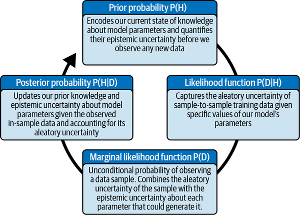
Figure 5-1. How the inverse probability rule builds upon knowledge with iterative probabilistic learning from data

Estimating the Probability of Debt Default

Let’s apply the PML mechanism discussed in the previous section to the problem of estimating the probability that a company might default on its debt. Assume you are an analyst at a hedge fund that buys high-yielding debt of companies with risky credit in the public credit markets because they often offer attractive risk-adjusted returns. These bonds are also known pejoratively as junk bonds because of their risky nature and the real possibility that these companies may not be able to pay back their bond holders.

Your fund’s analysts evaluate the credit risk of these companies using the company’s proprietary knowledge, experience, and management methods. When a portfolio manager estimates that there is only a 10% chance that a company might default, they buy its bonds at market prices that compensate the fund for the risk it is taking.

Your fund also uses conventional ML algorithms to search various data sources for information relating to the companies in their portfolio. These data might include earnings releases, press releases, analyst reports, credit market analyses, investor sentiment surveys, and the like. As soon as the ML classification model receives each piece of information that might affect a portfolio company, it immediately classifies the information as either a positive or negative rating for the company.

Over the years, your fund’s ML classification system has built a very valuable proprietary database of the vital information characteristics or features of these risky corporate borrowers. In particular, it has found that companies that eventually default on their debt accumulate 70% negative ratings. However, the companies that do not eventually default only accumulate 40% negative ratings.

Say you have been asked by your portfolio manager to develop a PML model that takes advantage of these proprietary resources to evaluate continually the probabilities of debt default as soon as new information about a company is processed by the ML classification system. If you are successful in developing this PML model, your fund will have an edge in the timing and direction of its high-yield debt trading strategies.

Now assume that your ML classification system has just alerted you of a negative rating it has assigned to XYZ, a new company in the funds’ bond portfolio that you are charged with monitoring. How would you update the probability of default of XYZ company based on the new negative rating? Let’s apply the PML model to this simple problem as a way to learn the PML process that you would apply to real, complex trades and investments.

• The probabilities of XYZ company defaulting—P(default)—and not defaulting—P(no default)—on its debt obligations are the model’s parameters that you want to estimate.

• Negative and positive ratings about XYZ company comprise the data that will inform you and condition your parameter estimates.

• You assume that all ratings are independent of one another and also that all the ratings are being sampled from the same underlying statistical distribution.

• Since XYZ company is in your fund’s portfolio, your prior probability of default before seeing any negative or positive ratings is P(default) = 10%.

• This implies that the prior probability that XYZ will not default on its debt is P(no default) = 90%.

• The likelihood that you would observe a negative rating from your ML classification system if XYZ were to default eventually is P(negative | default) = 70%.

• The likelihood of XYZ not defaulting eventually despite a negative rating is P(negative | no default) = 40%.

It might seem odd that P(negative | default) + P(negative | no default) = 0.7 + 0.4 = 1.1. These two probabilities don’t add up to 1 because they are conditioned on two noncomplementary hypotheses about the portfolio company. It might be helpful to think of any portfolio company as being one of two types of weighted coins: a no-default coin and a default coin. No-default coins show their negative side 40% of the time. Default coins show their negative side 70% of the time. You are trying to figure out which one of the two types of weighted coins your portfolio manager has chosen from a bag filled with both two types of coins.

You want to estimate the posterior probability of default after observing a negative rating, P(default | negative), and in light of your institutional knowledge of credit risk management. You now have all the probabilities and information you need to create a PML model and apply the inverse probability rule. Let’s encode the solution in Python:

# Import Python libraries
import numpy as np
import pandas as pd

# Create a dataframe for your bond analysis
bonds = pd.DataFrame(index=['Default', 'No Default'])

# The prior probability of default
# P(Default) = 0.10 and P(No Default) = 0.90

bonds['Prior'] = 0.10, 0.90

# The likelihood functions for observing negative ratings
# P(Negative|Default) = 0.70 and P(Negative|No Default) = 0.40

bonds['Likeli_Neg'] = 0.70, 0.40

# Joint probabilities of seeing a negative rating depending on 
# default or no default
# P(Negative|Default) * P(Default) and P(Negative|No Default) * P(No Default)

bonds['Joint1'] = bonds['Likeli_Neg'] * bonds['Prior']

# Add the joint probabilities to get the marginal likelihood or unconditional 
# probability of observing a negative rating
# P(Negative) = P(Negative|Default) * P(Default) + P(Negative|No Default) 
             * P(No Default)

prob_neg_data = bonds['Joint1'].sum()

# Use the inverse probability rule to calculate the updated probability of
# default based on the new negative rating and then print the data table.

bonds['Posterior1'] = bonds['Likeli_Neg'] * bonds['Prior']/prob_neg_data
bonds.round(2)

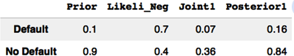
Based on our code, you can see the posterior probability of default of company XYZ given it has just received a negative rating P(default | negative) = 16%. The probability of default has risen from our prior probability of 10%, as would be expected.

Say a few days later your ML classifier alerts you to another negative rating about XYZ company. How do you update the probability of default now? The PML process is exactly the same. But now our prior probability of default is our current posterior probability of default, calculated previously. This is one of the most powerful features of the PML model: it learns dynamically by continually integrating our prior knowledge with new data in a mathematically rigorous manner. Let’s continue to code our solution to demonstrate this:

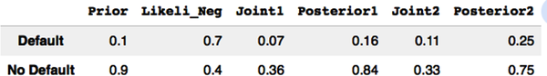
#Our new prior probability is our previous posterior probability, Posterior1. 
#Compute and print the table.

bonds['Joint2'] = bonds['Likeli_Neg'] * bonds['Posterior1']
prob_neg_data = bonds['Joint2'].sum()
bonds['Posterior2'] = bonds['Likeli_Neg'] * bonds['Posterior1']/prob_neg_data
bonds.round(2)

# Create a new table so that you can plot a graph with the appropriate information
table = bonds[['Prior', 'Posterior1', 'Posterior2']].round(2)

# Change columns so that x axis is the number of negative ratings
table.columns = ['0', '1', '2']

# Select the row to plot in the graph and print it.
default_row = table.iloc[0]
default_row.plot(figsize = (8,8), grid = True, 
xlabel = 'Updates based on recent negative ratings', 
ylabel = 'Probability of default', title = 'XYZ Bonds');

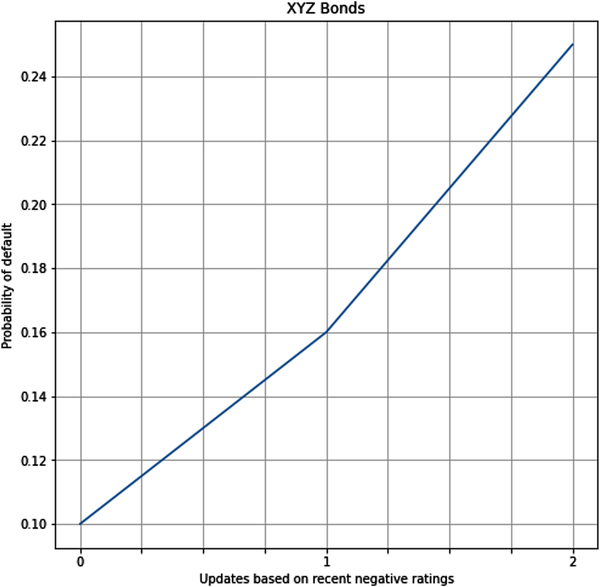
The probability of default given two negative ratings, P(default | 2 negatives), has gone up substantially to 25% in light of new information about the company, and its probability of default is approaching the fund’s risk limit. You decide to bring these results to the attention of the portfolio manager, who can do a more in-depth, holistic analysis of XYZ company and the current market environment.

It is important to note that PML models can ingest data one point at a time or all at once. The resulting final posterior probability will be the same regardless of the order in which the data arrives. Let’s verify this claim. Let’s assume instead that the fund’s ML classifier spat out two negative ratings of XYZ company within minutes.

• Assume again that the ratings of the ML classification system are independent and sampled from the same distribution as before.

• The probability of two consecutive negative ratings given that XYZ will default, P(2 negatives | default), is computed using the product rule for independent events:

  • P(2 negatives | default) = P(negative | default) × P(negative | default) = 0.70 × 0.70 = 0.49

• Similarly, probability of two negative ratings is computed given that XYZ will not default eventually: P(2 negatives | no default) = 0.40 × 0.40 = 0.16.

• The marginal likelihood or unconditional probability of observing two negative ratings for XYZ company is a weighted average over both possibilities of the company meeting its debt obligations:

  • P(2 negatives) = P(2 negatives | default) × P(default) + P(2 negatives | no default) × P( no default)

  • Plugging in the numbers for P(2 negatives) = (0.49 × 0.1) + (0.16 × 0.9) = 0.193

• Therefore, the posterior probability of XYZ company defaulting given two consecutive negative ratings is found:

  • P(default | 2 negatives) = P(2 negatives | default) × P(default) / P(2 negatives)

  • Plugging in the numbers for P(default | 2 negatives) = 0.049/0.193 = 0.25 or 25%

This is the same posterior probability we calculated for posterior2 in the Python code.

Generating Data with Predictive Probability Distributions

As was mentioned in Chapter 1, PML models are generative models that learn the underlying statistical structure of the data. This enables them to simulate new data seamlessly, including generating data that might be missing or corrupted. Most importantly, a PML model enables forward uncertainty propagation of its model’s outputs. It does this through its prior and posterior predictive distributions, which simulate potential data that a PML model could generate in the future and that are consistent with observed training data, model assumptions, and prior knowledge.

It is important to note that the prior and posterior distributions are probability distributions for inferring the distributions of our model’s parameters before and after training, respectively. They enable inverse uncertainty propagation. In contrast, the prior and posterior predictive distributions are probability distributions of our model for generating new data before and after training, respectively. They enable forward uncertainty propagation.

The prior and posterior predictive distributions combine two types of uncertainty: the aleatory uncertainty of sample-to-sample data simulated from its likelihood function; and the epistemic uncertainty of its parameters encoded in its prior and posterior probability distributions. Let’s continue to work on the example in the previous section to illustrate and explore these two predictive distributions.

The prior predictive distribution P(D′) is the prior probability distribution of simulated data (D′) we expect to observe in the training data (D) before we actually start training our model. The prior predictive distribution P(D′) does this by averaging the likelihood function P(D′ | H) over the prior probability distribution P(H) of the parameters.

Our PML model includes assumptions, constraints, likelihood functions, and prior probability distributions. The prior predictive distribution serves as a check on the appropriateness of our PML model before training begins. In essence, the prior predictive distribution P(D′) is retrodicting the training data (D) so that we can assess our model’s readiness for training. See Figure 5-2.

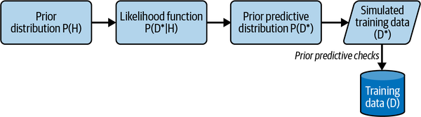
Figure 5-2. The prior predictive distribution generates new data before training. This simulated data is used to check if the model is ready for training.

If the actual training data (D) do not fall within a reasonable range of the simulated data (D′) generated by our prior predictive distribution, we should consider revising our model, starting with the prior probability distribution and then the likelihood function.

In the previous section, we already calculated the prior predictive mean of a negative rating, P(negative), as an expected value or weighted average mean when we calculated its marginal likelihood of observing a negative rating:

• P(negative) = P(negative | default) × P(default) + P(negative | no default) × P( no default)
• P(negative) = (0.70 × 0.10) + (0.40 × 0.90) = 0.43

We can similarly work out the prior predictive mean of a positive rating, P(positive), by using the complement of the negative likelihood functions.

• P(positive | default) = 1 – P(negative | default) and
• P(positive | no default) = 1 – P(negative | no default).
• Using these probabilities to compute the marginal likelihood function and plugging in the numbers, we get:
• P(positive) = P(positive | default) × P(default) + P(positive | no default) × P( no default)
• P(positive) = (0.30 × 0.10) + (0.60 × 0.90) = 0.57

In general, the prior predictive distribution is computed as follows:

• P(D′) = ${\sum }_{i}P\left(D^{\text{'}}\right|H_i)\times P\left(H_i\right)$ for discrete functions
• P(D′) = $\int P\left(D^{\text{'}}\right|H)\times P\left(H\right)dH$ for continuous functions

Note that there is a difference between the marginal likelihood function and the prior predictive distribution, even though the formulas look the same. The marginal likelihood function is the expected value of observing a specific data sample (D), such as a negative rating. The prior predictive distribution is a probability distribution that gives you the unconditional probability of any possible data (D′) within its sample space before any observations have actually been made. In our example, it gives you the unconditional probabilities of observing a negative and a positive rating for a portfolio company before you actually begin monitoring the company.

Posterior predictive distribution P(D″ | D) simulates the posterior probability distribution of out-of-sample or test data (D″) we expect to observe in the future after we have trained our model on the training data (D). It simulates test data samples (D″) by averaging the likelihood function P(D″ | H) over the posterior probability distribution P(H|D). In essence, the trained posterior predictive distribution P(D″ | D) is predicting the unseen test data (D^) so that we can assess our model’s readiness for testing. See Figure 5-3.

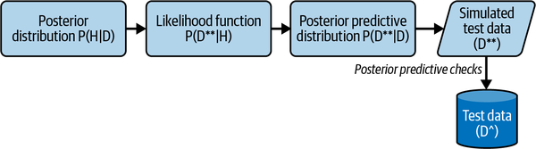
Figure 5-3. The posterior predictive distribution generates new data after training. This simulated data is used to check if the model is ready for testing.

Note that after we have trained our PML model on the in-sample data (D) and captured its aleatory uncertainty by using the likelihood function P(D|H), our posterior distribution P(H|D) gives us a better estimate of our parameter (H) and its epistemic uncertainty compared to our prior distribution P(H). Our likelihood function P(D″| H) continues to express the aleatory uncertainty of observing the out-of-sample data (D″).

The posterior predictive distribution serves as a final model check in the test environment. We can evaluate the usefulness of our model based on how closely the out-of-sample data distribution follows the data distribution predicted by the posterior predictive probability distribution.

In general, the posterior predictive distribution is given by the following formulas:

• P(D″ | D) = ${\sum }_{i}P\left(D^{\text{'}\text{'}}\right|H_i)\times P\left(H_i\right|D)$ for discrete functions
• P(D″ | D) = $\int P\left(D^{\text{'}\text{'}}\right|H)\times P\left(H\right|D)dH$ for continuous functions

The probability of observing another negative rating for XYZ company, given that we have already observed two negative ratings, needs to be updated. While it is still the expected value of generating another negative rating as before, the weights assigned to each parameter value are provided by the posterior probability distribution conditioned on observing two negative ratings. This is called the posterior predictive mean and is calculated as follows:

• P(negative | 2 negatives) = P(negative | default) × P(default | 2 negatives) + P(negative | no default) × P(no default | 2 negatives) = (0.7 × 0.25) + (0.4 × 0.75) = 0.475 or 47.5%

What is the probability of observing a positive rating for XYZ company now that we have observed two negative ratings? Since the posterior predictive distribution is a probability distribution, it follows that P(positive | 2 negatives) = 1 − P(negative | 2 negatives) = 0.525 or 52.5%. You can check for yourself that this is true by working through the probabilities as we have done in the previous sections.

Summary

In this chapter, we investigated the specific terms of the inverse probability rule and how they support a comprehensive PML framework discussed in Chapter 1. Specifically, the following terms of the rule enable continual knowledge integration and inverse uncertainty propagation:

• The prior probability distribution P(H) encodes our current knowledge and epistemic uncertainty about our model’s parameters before we observe any in-sample or training data.

• The likelihood function P(D|H) captures the data distribution and aleatory uncertainty of sample-to-sample training data we observe given a specific value of our model’s parameters.

• The marginal likelihood function P(D) gives us the unconditional probability of observing a specific sample by averaging over all possible parameter values, weighted by their prior probabilities. It combines the aleatory uncertainty of the observed sample data with the epistemic uncertainty about each parameter that might have generated that sample. It is a generally intractable constant that normalizes the posterior probability distribution so that it integrates to 1.

• The posterior probability distribution P(H|D) updates the estimates of our model’s parameters by integrating our prior knowledge about them with how plausible it is for each parameter to have generated the in-sample data that we actually observe. It is the target probability distribution that interests us most as it encodes the probabilistic learning of our model’s parameters, including their aleatory and epistemic uncertainties.

The prior and posterior predictive distributions enable forward uncertainty propagation of our PML model. They also act as checks on the usefulness of our models:

• The prior predictive distribution P(D′) gives us the unconditional probabilities of observing hypothetical in-sample training data (D′) before we actually begin our experiment and observe them. Note that this is not the actually observed in-sample data D.

• The posterior predictive distribution P(D″|D) gives us the conditional probabilities of observing hypothetical out-of-sample test data (D″) after our PML model has learned its parameters from in-sample training data (D).

It is important to note that the prior P(H) and posterior distributions P(H | D) give us the probability distributions about our model’s parameters before and after training our model on in-sample data D, respectively.

The prior predictive P(D′) and posterior predictive P(D″ | D) distributions give us the data-generating probability distributions of simulated in-sample (D′) and out-of-sample data (D″) before and after training our model on in-sample data D, respectively.

These powerful mechanisms enable dynamic, iterative, and integrative machine learning conditioned on data while quantifying both the aleatory and epistemic uncertainties of those learnings. The PML model enables both inference of model parameters and predictions based on those parameters conditioned on data. It seamlessly integrates inverse uncertainty propagation and forward uncertainty propagation in a logically consistent and mathematically rigorous manner while continually ingesting new data. This provides rock solid support for sound, dynamic, data-based decision making and risk management.

In the next chapter, we explore one of the most important features of PML models, especially for finance and investing. What puts PML models in a class of their own is that they know what they don’t know and calibrate their epistemic uncertainty accordingly. This leads us away from potentially disastrous and ruinous consequences of traditional ML systems that are extremely confident regardless of their ignorance. Adapting a famous line from Detective “Dirty” Harry, an iconic movie cop: a model’s got to know its limitations.

Further Reading

Downey, Allen B. “Bayes’s Theorem.” In Think Bayes: Bayesian Statistics in Python, 2nd ed. O’Reilly Media, 2021.

Jaynes, E. T. Probability Theory: The Logic of Science. Edited by G. Larry Bretthorst. New York: Cambridge University Press, 2003.

McElreath, Richard. “Small Worlds and Large Worlds.” In Statistical Rethinking: A Bayesian Course with Examples in R and Stan, 19–48. Boca Raton, FL: Chapman and Hall/CRC, 2016.

Ross, Kevin. “Introduction to Prediction.” In An Introduction to Bayesian Reasoning and Methods. Bookdown.org, 2022. https://bookdown.org/kevin_davisross/bayesian-reasoning-and-methods/.