Chapter 6. The Dangers of Conventional AI Systems
A man’s got to know his limitations.
—Detective “Dirty” Harry in the movie Magnum Force, as he watches an overconfident criminal mastermind’s car explode
A model’s got to know its limitations. This is worth emphasizing because of the importance of this characteristic for models in finance and investing. The corollary is that an AI’s got to know its limitations. The most serious limitation of all AI systems is that they lack common sense. This stems from their inability to understand causal relationships. AI systems only learn statistical relationships during training that are hard to generalize to new situations without comprehending causality.
In Chapter 1, we examined the three ways in which financial markets can humble you even when you apply our best models cautiously and thoughtfully. Markets will almost surely humiliate you when your models are based on flawed financial and statistical theories such as those discussed in the first half of the book. That’s actually not such a bad outcome, because a humiliating financial loss can often lead to personal insights and growth. A worse outcome is getting fired from your job or your career coming to an ignoble end. The worst outcome is personal financial ruin, where the wisdom gained from such an experience may not be timely enough to be useful.
When traditional ML models (such as deep learning networks and logistic regression) are trained, they generally use the maximum likelihood estimation (MLE) method to learn the model parameters from in-sample data. Consequently, these ML systems have three deep flaws that severely limit their use in finance and investing. First, the parameter estimates of their models are erroneous when used with small datasets, especially when they learn from noisy financial data. Second, these ML models are awful at extrapolating beyond the data ranges and classes on which they have been trained and tested. Third, the probability scores of MLE models have to be calibrated into valid probabilities by using a function such as a Sigmoid or Softmax function. However, these calibrations are not guaranteed to represent the underlying probabilities accurately leading to poor uncertainty quantifications.
What makes all these flaws egregious is that the conventional statistical models on which these ML systems are based make erroneous estimates and predictions with appallingly high confidence, making them very dangerous in an uncertain world. Just like in the movie Magnum Force, these overconfident AI models have the potential of blowing up investment accounts, companies, financial institutions, and economies if they are implemented without understanding their severe limitations.
In Chapter 4, we exposed the fallacious inferential reasoning of popular statistical methods such as NHST, p-values, and confidence intervals. In this chapter, we examine the severe limitations and flaws of the popular MLE method and why it fails in finance and investing. We do this by examining a case where we want to project whether a newly listed public company we have invested in will beat its quarterly earnings expectations, based on a short track record. By comparing the results of a traditional MLE model with that of a probabilistic model, we demonstrate why probabilistic models are better suited for finance and investing in general, especially when datasets are sparse.
As discussed earlier, most real-world probabilistic inference problems cannot be solved analytically because of the intractable complexity of the summations/integrals in the marginal probability distribution. Instead of using flawed probability calibration methods used by MLE models, we settle for approximate numerical solutions to probabilistic inference problems. Even though the earnings expectation problem can be solved analytically using basic calculus, we apply grid approximation to solve it to show how this simple, powerful technique works and makes probabilistic inference much easier to understand.
Markov chain Monte Carlo (MCMC) simulation is a breakthrough numerical method that has transformed the usability of probabilistic inference by estimating analytically intractable, high dimensional posterior probability distributions. MCMC simulates complex probability distributions using dependent random sampling algorithms. We explore the fundamental concepts underlying this powerful, scalable simulation method. As a proof-of-concept of the MCMC method, we use the famous Metropolis sampling algorithm to simulate a Student’s t-distribution with fat tails.
AI Systems: A Dangerous Lack of Common Sense
Humans are endowed with a very important quality that no AI has been able to learn so far: a commonsensical ability to generalize our learnings reasonably well to unseen, out-of-sample related classes or ranges, even if we have not been specifically trained on them. Unlike AI systems, almost all humans can easily deduce, infer, and adjust their knowledge to new circumstances based on common sense. For instance, a deep neural network trained to recognize live elephants in the wilderness was unable to recognize a taxidermy elephant on display in a museum.1 Even a toddler could do this task easily by just using their common sense. As others have pointed out, the AI system literally could not see the elephant in the room!
The primary reason for such common failures is that AI models only compute correlations and don’t have the tools to comprehend causation. Furthermore, humans are able to abstract concepts from specific examples and think in terms of generalization of objects and causal relationships among them, while AI systems are just unable to do that. This is a major problem when dealing with noisy, big datasets as they present abundant opportunities for correlating variables that have no plausible physical or causal relationship. With large datasets, spurious correlations among variables are the rule, not the exception.
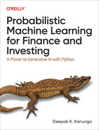
For instance, Figure 6-1 shows that between 1999 and 2009, there was a 99.8% correlation between US spending on science, space and technology, and suicides by hanging, strangulation, and suffocation.2
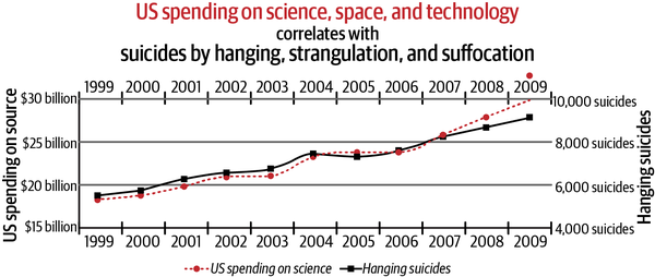
Figure 6-1. Spurious correlations are the rule in big datasets3
Clearly this relationship is nonsensical and underscores the adage that correlation does not imply causation. Humans would understand the absurdity of such spurious correlations quite easily, but not AI systems. This also makes AI systems easy to fool by humans who understand such weaknesses and can exploit them.
While artificial neural networks were inspired by the structure and function of the human brain, our understanding of how human neurons learn and work is still incomplete. As a result, artificial neural networks are not exact replicas of biological neurons, and there are still many unsolved mysteries surrounding the workings of the human brain. The term “deep neural networks” is a misleading marketing term to describe artificial neural networks with more than two hidden layers between the input and output layers. There is nothing deep about a deep neural network that lacks the common sense of a toddler.4
Why MLE Models Fail in Finance
The MLE statistical method is used by all conventional parametric ML systems, from simple linear models to complex deep learning neural networks. The MLE method is used to compute the optimal parameters that best fit the data of an assumed statistical distribution. The MLE algorithm is useful when the model is dealing with only aleatory uncertainty of large datasets that have time-invariant statistical distributions where optimization makes sense.
Much valuable information and assessment of uncertainty are lost when a statistical distribution is summarized by a point estimate, even if it is an optimal estimate. By definition and design, a point estimate cannot capture the epistemic uncertainty of model parameters because they are not probability distributions. This has serious consequences in finance and investing, where we are dealing with complex, dynamic social systems that are steeped in all three dimensions of uncertainty: aleatory, epistemic, and ontological. In Chapter 1, we discussed why it is dangerous and foolish to use point estimates in finance and investing given that we are continually dealing with erroneous measurements, incomplete information, and three-dimensional uncertainty. In other words, MLE-based traditional ML systems operate only along one dimension in the three-dimensional space of uncertainty as illustrated in Figure 2-7. What is even more alarming is that many of these ML systems are generally black boxes operating confidently at high speeds with flawed probability calibrations.
Furthermore, MLE ignores prior domain knowledge in the form of base rates or prior probabilities, which can lead to base-rate fallacies, as discussed in Chapter 4. This is especially true when MLE is applied to small datasets. Let’s actually see why this is indeed the case by applying the MLE method to a real-world problem of estimating the probability that a company will actually beat the market’s expectation of its earnings estimates based on a short track record. This example has been inspired by the coin tossing example illustrated in the book referred to in the references.5
An MLE Model for Earnings Expectations
Assume you have changed jobs and are now working at a mutual fund as an equity analyst. Last year, your fund was allocated equity shares in the initial public offering (IPO) of ZYX, a high-growth technology company. Even though ZYX has never turned a profit in its entire nascent life, its brand is already a household name due in large part to its aggressive marketing campaigns that were supported by massive amounts of venture capital. Clearly, private and public equity investors bought into its compelling growth story, as narrated by its charismatic CEO.
In all the last three quarters since its IPO, the negative earnings of ZYX beat market expectations of even bigger losses. In financial markets, less bad is good. The stock price of ZYX has continued its relentless climb upward and is currently trading at all-time highs, enriching everyone in the process. Your portfolio manager (PM) has asked you to estimate the probability that ZYX’s earnings will beat market expectations in the upcoming fourth quarter. Based on your probability estimate, your PM is going to increase or decrease the fund’s equity investment in ZYX before their earnings announcement, which is due shortly.
Having been schooled in conventional statistical methods, we decide to build a standard MLE model to compute the required probability. The earnings announcement event has only two outcomes that interest us: either the earnings beat market expectations, or they fall short of them. We don’t care about the outcome of earnings merely meeting market expectations. Like many other investors, your PM has decided that such an outcome is the equivalent of earnings falling short of market expectations. It is common knowledge that management of companies play a game with Wall Street analysts throughout the year, where they lower their earnings expectations so that it becomes easier to beat those expectations when the actual earnings are announced.
Let’s design our quarterly earnings MLE model and specify the assumptions that underpin it:
In a single event or trial, the model’s output variable y can assume only one of two possible outcomes, y = 1 or y = 0.
The two outcomes are mutually exclusive and collectively exhaustive.
Assign y = 1 to the outcome that ZYX beats market expectations of its quarterly earnings.
Assign y = 0 to the outcome that ZYX does not beat or only meets market expectations of its quarterly earnings.
We now have to select a statistical distribution for our likelihood function that best models the binary event of an earnings announcement. The Bernoulli distribution models a single event or trial that has binary outcomes. See Figure 6-2.
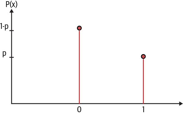
Figure 6-2. Bernoulli variable6 with outcome x = 1 occurring with probability p and outcome x = 0 occurring with probability 1-p
Recall that in Chapter 1, we used the binomial distribution to model the total number of interest rate increases by the Federal Reserve over several meetings or trials. The Bernoulli distribution is a special case of the binomial distribution since they both have the same probability distribution when used for a single trial.
Assume that variable y follows a Bernoulli distribution with an unknown parameter p, which gives us the probability of an earnings beat (y = 1).
Since both probabilities must add up to 1, this implies that the probability of not beating earnings expectations (y = 0) is its complement, 1-p.
Our objective is to find the MLE of the parameter p, the probability that ZYX beats the market expectations of its quarterly earnings based on ZYX’s short track record of setting market expectations and then beating them.
A Bernoulli process of the variable y is a discrete time series of independent and identically distributed (i.i.d.) Bernoulli trials, denoted by yi.
The i.i.d. assumption means that each earnings announcement is independent of all the previous ones and is drawn from the same Bernoulli distribution with constant parameter p.
In its last three quarters, ZYX beat earnings expectations, so our training data for parameter p is D = (y1 = 1, y2 = 1, y3 = 1).
Let’s call p′ the MLE for the parameter p of the Bernoulli variable y. It can be shown mathematically that p′ is the expected value or arithmetic mean of the sample of time series data D. It is the optimal parameter that when inserted in a Bernoulli likelihood function best fits the time series data D. This implies p′ trained on dataset D is:
p′(D) = (y1+y2+y3) / 3 = (1 + 1 + 1) / 3 = 3 / 3 = 1
Therefore, the probability that ZYX will beat market expectations of its earnings in its fourth quarter is P(y4 = 1 | p′) = p′ = 1 or 100%.
Since MLE models only allow aleatory uncertainty caused by random sampling of data, let’s compute the variance of y. The variance of a Bernoulli variable y with parameter p′ is given by:
Aleatory uncertainty or variance (y | p′) = (p′) × (1 – p′) = 1 × (1 – 1) = 1 × 0 = 0.
Epistemic uncertainty = 0 since p′ is a point estimate that is an optimum.
Ontological uncertainty = 0 since p′ is considered a “true” constant and the Bernoulli distribution is assumed to be time invariant.
So our MLE model is assigning a 100% probability with a 0 sampling error that y4 = 1. In other words, our model is absolutely certain that ZYX is going to beat market expectations of its earnings estimate in the upcoming fourth quarter. Our model’s heroic prediction of ZYX’s earnings beating market expectations is based on only three data points of a fledgling, loss-making technology company. Moreover, our current MLE model will continue to predict an earnings beat for every quarterly earnings event for the rest of ZYX’s life. It’s not just death and taxes that are certain. We need to add our MLE model’s predictions to the list.
Any financial analyst with even a modicum of common sense would not present this MLE model and its predictions to their portfolio manager. However, it is very common to have sparse datasets in finance and investing. For instance, we have financial data for only two occurrences of global pandemics. Early stage technology startup companies or strategy/special projects have little or no relevant data for making specific decisions. Since the Great Depression ended in 1933, the US economy has experienced only 13 recessions. Since 1942, the S&P 500 has had three consecutive years of negative total returns only once (2000–2003). These are some of the obvious examples. The list of sparse datasets in finance and investing is quite long indeed.
Clearly, MLE models are dangerous when applied to sparse datasets common in finance and investing. They really don’t know their limitations and unabashedly flaunt their ignorance. Building complex financial ML systems based on MLE models will only lead to financial disasters sooner rather than later.
A Probabilistic Model for Earnings Expectations
Now let’s delete our useless MLE model and pause to reflect on the problem. With only three data points to work with, it would be foolhardy to be absolutely certain about any point estimate of the parameter p, the probability that ZYX’s fourth quarter earnings will beat market expectations. Why is that? There are so many possible things that could have gone wrong in the past quarter that only some company insiders might be aware of. Given the persistent asymmetry of information between the company management and its shareholders, this is always possible. This is a major source of our epistemic uncertainty about parameter p.
Most importantly, there are so many things—company specific, political, regulatory, legal, monetary, and economic—that can go wrong in the immediate future and change the market’s expectations before ZYX makes its earnings public. These are some of the sources of our ontological uncertainty. Of course, nobody knows what will happen in the future, but it is more likely that the future will reflect the recent past than not.
So based on our understanding of the three dimensions of uncertainty of the real world we live in and the information that we currently have, we can reasonably bet that it is very probable that ZYX will beat the market’s expectations of its fourth quarter earnings. However, it’s not a certainty. This implies that our model parameter p should be able to take any value between 0 and 1, with the ones closer to 1 being more probable. In other words, our estimate for p is better expressed by a probability distribution than as any particular point estimate. In particular, after seeing the dataset D, our estimate for p is best expressed as a positively skewed probability distribution.
Note that the MLE is the optimal value for p that best replicates the observed data. But there is no universal natural law that says that it is a certainty that the MLE is the value of p that produced the in-sample data. Other values of the parameter p could easily have generated the dataset D too. We are dealing with complex social systems with emotional beings that do suboptimal things all the time. Most importantly, we are not constrained by the problem to pick only one value for p.
Let’s actually quantify and visualize the statistical distribution for p more precisely by building a probabilistic model. Recall that a probabilistic model requires us to specify two probability distributions:
The first is a prior probability distribution P(p) that encapsulates our knowledge or hypothesis about model parameters before we observe any data. Let’s assume you have no prior knowledge about ZYX company or any idea of what the parameter p should be. This makes a uniform distribution, U(0, 1), that we learned in the Monty Hall problem a good choice for our prior distribution. This distribution assigns equal probability to all values of p between 0 and 1. So P(p) ~U (0, 1), where the tilde sign (~) is shorthand for “is statistically distributed as.”
The second is a likelihood function P(D | p) that gives us the plausibility of observing our in-sample data D assuming any value for our parameter p between 0 and 1. We will continue to use the Bernoulli probability distribution and its related process in our probabilistic model. So the likelihood function of our probabilistic model is P(D | p) ~Bernoulli (p).
Our objective is to estimate the posterior probability distribution of our model parameter p given the in-sample data D and our prior knowledge or hypothesis of p. This will give us the probability distribution for the outcome y = 1, the probability of an earnings beat. As always, we will use the inverse probability rule to compute the probability distribution of p given the data D. Our probabilistic model can be specified as follows:
P( p | D) = P(D | p) ✕ P(p) / P(D) where
P(p) ~U (0, 1)
P(D | p) ~ Bernoulli (p)
D = (y1 = 1, y2 = 1, y3 = 1)
This posterior distribution is simple enough to be solved analytically using basic calculus.7 However, this involves using integrals over probability density functions, which may not be accessible to many readers. Instead of doing that here, we will compute the posterior distribution using a simple numerical approach called grid approximation. This approach will convert our problem of integral calculus into a much simpler problem of descriptive statistics. This should help us to build our intuition for the underlying mechanism of our probabilistic model.
Since our prior distribution is discrete and uniformly distributed, we can split the interval between 0 and 1 into 9 equidistant points, 0.1 apart, as shown in Figure 6-3.
Figure 6-3. There are n number of grid points uniformly distributed between a and b, and each has a probability of 1/n8
So our grid points are {p1 = 0.1, p2 = 0.2, .., p9 = 0.9}. Since the n grid points are uniformly distributed, they all have the same probability, namely P(p) = 1/n, where n is the number of grid points. In our approximation, we have n = 9 grid points.
The prior probability for every parameter p1,...p9 on our one-dimensional grid is P(p) = 1/9 = 0.111.
For every parameter pi we sample from the set of nine grid points to simulate an earnings event with a value of pi, the Bernoulli likelihood function generates y = 1 with probability pi or y = 0 with probability 1-pi. The Bernoulli process for the last three quarters of ZYX’s earnings event is given by our training data D = (y1 = 1, y2 = 1, y3 = 1). So the likelihood of the Bernoulli process is:
P(D | pi) = pi × pi × pi = pi3
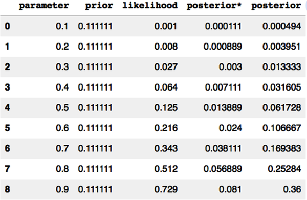
For each parameter pi, we use a grid point {p1,...p9} to compute the unnormalized posterior distribution P*(p | D), using the inverse probability rule. To compute the normalized posterior P(p | D), we first add up the all the unnormalized posterior values and then divide each unnormalized posterior by the sum as follows:
P(pi | D) =
Let’s use Python code to develop a grid approximation of the solution:
# Import the relevant Python librariesimportnumpyasnpimportpandasaspdimportmatplotlib.pyplotasplt# Create 9 grid points for the model parameter, from 0.1 to 0.9 spaced 0.1 apartp=np.arange(0.1,1,0.1)# Since all parameters are uniformly distributed and equally likely, the# probability for each parameter = 1/n = 1/9prior=1/len(p)# Create a pandas DataFrame with the relevant columns to store# individual calculationsearnings_beat=pd.DataFrame(columns=['parameter','prior','likelihood','posterior*','posterior'])# Store each parameter valueearnings_beat['parameter']=p# Loop computes the unnormalized posterior probability distribution# for each value of the parameterforiinrange(0,len(p)):earnings_beat.iloc[i,1]=prior# Since our training data has three earnings beats in a row,# each having a probability of pearnings_beat.iloc[i,2]=p[i]**3# Use the unnormalized inverse probability ruleearnings_beat.iloc[i,3]=prior*(p[i]**3)# Normalize the probability distribution so that all values add up to 1earnings_beat['posterior']=earnings_beat['posterior*']/sum(earnings_beat['posterior*'])# Display the data frame to show each calculationearnings_beat
# Plot the prior and posterior probability distribution for the model parameterplt.figure(figsize=(16,6)),plt.subplot(1,2,1),plt.ylim([0,0.5])plt.stem(earnings_beat['parameter'],earnings_beat['prior'],use_line_collection=True)plt.xlabel('Model parameter p'),plt.ylabel('Probability of parameter P(p)'),plt.title('Prior distribution of our model parameter')plt.subplot(1,2,2),plt.ylim([0,0.5])plt.stem(earnings_beat['parameter'],earnings_beat['posterior'],use_line_collection=True)plt.xlabel('Model parameter p'),plt.ylabel('Probability of parameter P(p)'),plt.title('Posterior distribution of our model parameter')plt.show()
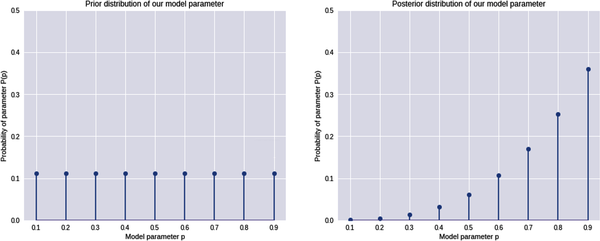
This figure clearly shows that our probabilistic model has computed a probability distribution for the model parameter p before and after training the model on in-sample data D. This is a much more realistic solution, given that we always have incomplete information about any event.
Our model has learned the parameter p from our prior knowledge and the data. This is only half the solution. We need to use our model to predict the probability that ZYX will beat the market’s expectations of its fourth quarter earnings estimates. In other words, we need to develop the predictive distributions of our model. Let’s continue coding that:
# Since P(yi=1|pi) = pi, we compute the probability weighted average of# observing y=1 using our prior probabilities as the weights# This probability weighted average gives us the prior predictive probability of# observing y=1 before observing any dataprior_predictive_1=sum(earnings_beat['parameter']*earnings_beat['prior'])# The prior predictive probability of observing outcome y=0 is the complement of# P(y=1) calculated aboveprior_predictive_0=1-prior_predictive_1# Since we have picked a uniform distribution for our parameter, our model# predicts that both outcomes are equally likely prior to observing any data(prior_predictive_0,prior_predictive_1)(0.5,0.5)# Since P(yi=1|pi) = pi, we compute the probability weighted average of# observing y=1 but now we use the posterior probabilities as the weights# This probability weighted average gives us the posterior predictive# probability of observing y=1 after observing in-sample dataD={y1=1,y2=1,y3=1}posterior_predictive_1=sum(earnings_beat['parameter']*earnings_beat['posterior'])# The posterior predictive probability of observing outcome y=0 is the# complement of P(y=1|D) calculated aboveposterior_predictive_0=1-posterior_predictive_1# After observing data D, our model predicts that observing y=1 is# about 3 times more likely than observing y=0round(posterior_predictive_0,2),round(posterior_predictive_1,2)(0.24,0.76)# Plot the prior and posterior predictive probability distribution# for the event outcomesplt.figure(figsize=(16,6)),plt.subplot(1,2,1),plt.ylim([0,1])plt.stem([0,1],[prior_predictive_0,prior_predictive_1],use_line_collection=True)plt.xlabel('Binary outcome for variable y'),plt.ylabel('Probability P(y)'),plt.title('Prior predictive distribution of an earnings beat')plt.subplot(1,2,2),plt.ylim([0,1])plt.stem([0,1],[posterior_predictive_0,posterior_predictive_1],use_line_collection=True)plt.xlabel('Binary outcome for variable y'),plt.ylabel('Probability P(y)'),plt.title('Posterior predictive distribution of an earnings beat')plt.show()
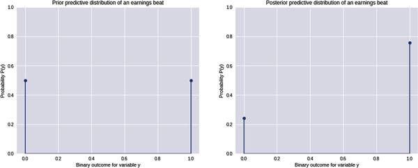
The expected value or posterior predictive mean is 76%, which is close to the theoretical value of 75%. Regardless, our probabilistic model is not 100% sure that ZYX will beat market expectations in the fourth quarter, even though it has successfully done so in the last three quarters. Our model predicts that it is about three times more likely to beat market expectations than not. This is a far more realistic probability distribution and something we can use to make our investment decisions.
Unfortunately, the numerical grid approximation technique we used to solve the earnings expectations problem does not scale if the model has more than a few parameters. So the most scalable and robust numerical methods that we are left with are random sampling methods for estimating approximate solutions for probabilistic inference problems.
Markov Chain Monte Carlo Simulations
Generally speaking, there are two types of random sampling methods: independent sampling, and dependent sampling. The standard Monte Carlo simulation (MCS) method that we learned in Chapter 3 is an independent random sampling method. However, random sampling does not work well when samples are dependent or correlated with one another.
Furthermore, these independent sampling algorithms are inefficient when the target probability distribution they are trying to simulate has many parameters or dimensions. We generally encounter these two issues when simulating complex posterior probability distributions. So we need random sampling algorithms which work with samples that are dependent or correlated with one another.9 Markov chains are a popular way of generating dependent random samples. The most important aspect of a Markov chain is that the next sample generated is only dependent on the previous sample and independent of everything else.
Markov Chains
A Markov chain is used to model a stochastic process consisting of a series of discrete and dependent states linked together in a chain-like structure. It is a sequential process that transitions probabilistically in discrete time from state to state in the chain. The most important aspect of a Markov state is that it is memoryless. For any state, its future state only depends on the transition probabilities of the current state and is independent of all past states and the path it took to get to its current state. It’s as if Markovian chains have encoded Master Oogway’s Zen saying from the movie Kung Fu Panda: “Yesterday is history, tomorrow is a mystery, but today is a gift. That is why it is called the present.”
Equally important, this simplifying memoryless property makes the Markovian chain easy to understand and implement. A random walk process, whether arithmetic or geometric, is a specific type of Markov chain and is used extensively to model asset prices, returns, interest rates, and volatility. A graphic representation of a Markov chain depicting the three basic and discrete states of the financial markets and their hypothetical transition probabilities is shown in Figure 6-4.
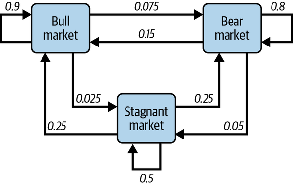
Figure 6-4. A Markov chain depicting the three basic states of the financial markets and their hypothetical transition probabilities10
According to this state transition diagram, if the financial market is currently in a bear market state, there is an 80% probability it will remain in a bear market state. However, there is a 15% probability that the market will transition to a bull market state and a 5% probability it will transition to a stagnant market state.
Say the market transitions from a bear market state to a stagnant market state and then to a bull market state over time. Once it is in the bull market state, it will have no dependence or memory of the stagnant market state or bear market state. Probabilities about its transition to its future state will be dependent only on its present bull market state. So, for example, there is a 90% probability that it will stay in a bull market state regardless of whether it came from a stagnant market state or a bear market state or some permutation of the two. In other words, the future state of any Markov chain is conditionally independent of all past states given the current state.
Despite the random walks a stochastic process takes in the state space of a Markov chain, if it can go from one state to every other state in a finite number of moves, the Markov chain is said to be stationary ergodic. Based on this definition, the Markov chain of the hypothetical financial market process depicted in Figure 6-3 is stationary ergodic because the market will eventually reach any state in the Markov chain given enough time. Such a hypothetical stationary ergodic financial market would imply that the ensemble average price returns of all investors is expected to equal the price returns of every single random trajectory taken by any single investor in the ensemble over a long enough time period.
However, as was discussed earlier, real financial markets are neither stationary nor ergodic. For instance, as an investor, you could suffer heavy losses in an unrelenting bear market state, or make foolish investments in a bubblicious bull market state, or be forced to liquidate your investments to pay for expensive divorce lawyers in a stagnant market state, and never be in another market state again. You would then be banished to a special Markovian state called an absorbing state from which there is no escape. This special state absorbs the essence of the lyric from the Eagles’ song “Hotel California”: “You can check out any time you like, but you can never leave.” We will discuss the problem of ergodicity in finance and investing in Chapter 8.
Metropolis Sampling
The Metropolis algorithm generates a Markov chain to simulate any discrete or continuous target probability distribution. The Metropolis algorithm iteratively generates dependent random samples based on three key elements:
- Proposal probability distribution
- This is a probability distribution that helps explore the target probability distribution efficiently by proposing the next state in the Markov chain based on the current state. Different proposal distributions can be used depending on the problem.
- Proposal acceptance ratio
- This is a measure of the relative probability of the proposed move. In a probabilistic inference problem, the acceptance ratio is the ratio of the posterior probabilities of the target distribution evaluated at the proposed state to the current state in the Markov chain. Recall from the previous chapter that taking the ratio of the posterior probabilities at two different points gets rid of the analytically intractable marginal probability distribution.
- Decision rules on the proposed state
- These are probabilistic decision rules that determine whether to accept or reject the proposed state in the chain. If the acceptance ratio is greater than or equal to 1, the proposed state is accepted and the Markov chain moves to the next state. If the acceptance ratio is less than 1, the algorithm generates a random number between 0 and 1. If the random number is less than the acceptance ratio, the proposed state is accepted. Otherwise it is rejected.
The Metropolis algorithm builds its Markov chain iteratively and stops when the required number of samples have been accepted. The accepted samples are then used to simulate the target probability distribution.
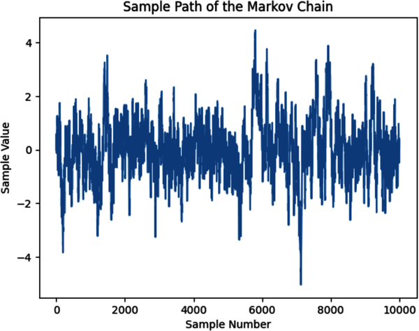
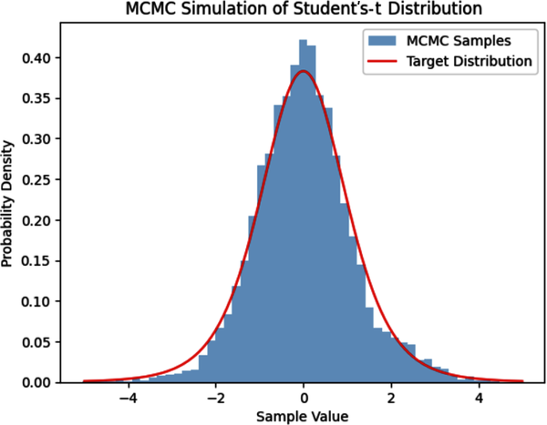
As a proof-of-concept of MCMC simulation, we will use the Metropolis algorithm to simulate a Student’s t-distribution with six degrees of freedom. This distribution is widely used in finance and investing for modeling asset price return distributions with fat tails. The Student’s t-distribution is a family of probability distributions, with each specific distribution controlled by its degrees of freedom parameter. The lower that value, the fatter the tails of the distribution. We will apply this distribution and discuss it further in the next chapter.
In the following Python code, we use the uniform distribution as the proposal distribution and the Student’s t-distribution with six degrees of freedom as our target distribution to simulate. It initializes the Markov chain arbitrarily at x = 0 and runs the Metropolis sampling algorithm 10,000 times. The resulting samples are stored in a list, which is plotted to visualize the sample path of the Markov chain. Finally, the code plots a histogram of the samples to show its convergence to the actual target distribution:
#Import Python librariesimportnumpyasnpimportscipy.statsasstatsimportmatplotlib.pyplotasplt# Define the target distribution - Student's t-distribution# with 6 degrees of freedom.# Use location=0 and scale=1 parameters which are the default# values of the Student's t-distribution# x is any continuous variabledeftarget(x):returnstats.t.(x,df=6)# Define the proposal distribution (uniform distribution)defproposal(x):# Returns random sample between x-0.5 and x+0.5 of the current valuereturnstats.uniform.rvs(loc=x-0.5,scale=1)# Set the initial state arbitrarily at 0 and set the number of# iterations to 10,000x0=0n_iter=10000# Initialize the Markov chain and the samples listx=x0samples=[x]# Run the Metropolis algorithm to generate new samples and store them in# the 'samples' listforiinrange(n_iter):# Generate a proposed state from the proposal distributionx_proposed=proposal(x)# Calculate the acceptance ratioacceptance_ratio=target(x_proposed)/target(x)# Accept or reject the proposed stateifacceptance_ratio>=1:# Accept new samplex=x_proposedelse:u=np.random.rand()# Reject new sampleifu<acceptance_ratio:x=x_proposed# Add the current state to the list of samplessamples.append(x)# Plot the sample path of the Markov chainplt.plot(samples)plt.xlabel('Sample Number')plt.ylabel('Sample Value')plt.title('Sample Path of the Markov Chain')plt.show()# Plot the histogram of the samples and compare it with the target distributionplt.hist(samples,bins=50,density=True,alpha=0.5,label='MCMC Samples')x_range=np.linspace(-5,5,1000)plt.plot(x_range,target(x_range),'r-',label='Target Distribution')plt.xlabel('Sample Value')plt.ylabel('Probability Density')plt.title('MCMC Simulation of Students-T Distribution')plt.legend()plt.show()
In 1970, William Hastings generalized the Metropolis sampling algorithm so that asymmetric proposal distributions and more flexible acceptance criteria could be applied. The resulting Metropolis-Hastings MCMC algorithm can simulate any target probability distribution asymptotically, i.e., given enough samples, the simulation will converge to the target probability distribution. However, this algorithm can be inefficient and costly for high-dimensional, complex target distributions.
The Metropolis-Hastings algorithm is dependent on the arbitrary initial starting value of the Markov chain. The initial samples gathered during this period, called the burn-in period, are generally discarded. The randomness of the walk-through state space can waste time due to the possibility of revisiting the same regions several times. Moreover, the algorithm can get stuck in narrow regions of multidimensional spaces.
Modern dependent sampling algorithms have been developed to address the shortcomings of this general-purpose MCMC sampling algorithm. The Hamiltonian Monte Carlo (HMC) algorithm uses the geometry of any continuous target distribution to move efficiently in high-dimensional space. It is the default MCMC sampling algorithm in the PyMC library, and we don’t need any specialized knowledge to use it. In the next chapter, we will use these MCMC algorithms to simulate the posterior probability distributions of model parameters.
Summary
Traditional statistical MLE models on which most conventional ML systems are based are limited in their capabilities. They are designed to deal with only aleatory uncertainty and are unaware of their limitations. As we have demonstrated in this chapter, MLE-based models make silly predictions confidently. This makes them dangerous in our world of three-dimensional uncertainty. Poor predictive performance and disastrous risk management from such overconfident, simplistic, and hasty ML models are almost surely inevitable in the complex world of finance and investing.
In designing probabilistic models, we acknowledge the fact that only death is certain—everything else, including taxes, has a probability distribution. Probabilistic models are designed to manage uncertainties generated from noisy sample data and inexact model parameters. These models enable us to go from a one-dimensional world of aleatory uncertainty to a two-dimensional world with aleatory and epistemic uncertainties. This makes them more appropriate for the world of finance and investing. However, this comes at the cost of higher computational complexities.
To apply probabilistic machine learning to complex financial and investing problems, we have to use dependent random sampling because other numerical methods don’t work or don’t scale. MCMC simulation methods are transformative. They use dependent random sampling algorithms to simulate complex probability distributions that are difficult to sample from directly. We will apply MCMC methods in the next chapter, using a popular probabilistic ML Python library.
Ontological uncertainty emanates from complex social systems, which can be disruptive at times. Among other things, it involves rethinking and redesigning the probabilistic model from scratch and making it more appropriate for the new market environment. This is generally best managed by human beings with common sense, judgment, and experience. We are still very much relevant in the bold, new world of AI and have, indeed, the hardest job.
References
Dürr, Oliver, and Beate Sick. Probabilistic Deep Learning with Python, Keras, and TensorFlow Probability. Manning Publications, 2020.
Guo, Chuan, Geoff Pleiss, Yu Sun, and Kilian Q. Weinberger. “On Calibration of Modern Neural Networks.” Last revised August 3, 2017. https://arxiv.org/abs/1706.04599.
Lambert, Ben. A Student’s Guide to Bayesian Statistics. London, UK: Sage Publications, 2018.
Mitchell, Melanie. Artificial Intelligence: A Guide for Thinking Humans. New York: Farrar, Straus and Giroux, 2020.
Vigen, Tyler. Spurious Correlations. New York: Hachette Books, 2015.
1 Oliver Dürr and Beate Sick, “Bayesian Learning,” in Probabilistic Deep Learning with Python, Keras, and TensorFlow Probability (Manning Publications, 2020), 197–228.
2 Tyler Vigen, Spurious Correlations (New York: Hachette Books, 2015).
3 Adapted from an image on Wikimedia Commons.
4 Melanie Mitchell, “Knowledge, Abstraction, and Analogy in Artificial Intelligence,” in Artificial Intelligence: A Guide for Thinking Humans (New York: Farrar, Straus and Giroux, 2019), 247–65.
5 Dürr and Sick, “Bayesian Learning.”
6 Adapted from an image on Wikimedia Commons.
7 Dürr and Sick, “Bayesian Learning.”
8 Adapted from an image on Wikimedia Commons.
9 Ben Lambert, “Leaving Conjugates Behind: Markov Chain Monte Carlo,” in A Student’s Guide to Bayesian Statistics (London, UK: Sage Publications, 2018), 263–90.
10 Adapted from an image on Wikimedia Commons.