Chapter 2. Analyzing and Quantifying Uncertainty
There are known knowns. These are things we know that we know. There are known unknowns. That is to say, there are things that we know we don’t know. But there are also unknown unknowns. There are things we don’t know we don’t know.
—Donald Rumsfeld, Former US Secretary of Defense
The Monty Hall problem, a famous probability brainteaser, is an entertaining way to explore the complex and profound nature of uncertainty that we face in our personal and professional lives. More pertinently, the solution to the Monty Hall problem is essentially a betting strategy. Throughout this chapter, we use it to explain many key concepts and pitfalls in probability, statistics, machine learning, game theory, finance, and investing.
In this chapter, we will solve the apparent paradox of the Monty Hall problem by developing two analytical solutions of differing complexity using the fundamental rules of probability theory. We also derive the inverse probability rule that is pivotal to probabilistic machine learning. Later in this chapter, we confirm these analytical solutions with a Monte Carlo simulation (MCS), one of the most powerful numerical techniques that is used extensively in finance and investing.
There are three types of uncertainty embedded in the Monty Hall problem that we examine. Aleatory uncertainty is the randomness in the observed data (the known knowns). Epistemic uncertainty arises from the lack of knowledge about the underlying phenomenon (the known unknowns). Ontological uncertainty evolves from the nature of human affairs and its inherently unpredictable dynamics (the unknown unknowns).
Probability is used to quantify and analyze uncertainty in a systematic manner. In doing so, we reject the vacuous distinction between risk and uncertainty. Probability is truly the logic of science. It might be surprising for you to know that we can agree on the axioms of probability theory, yet disagree on the meaning of probability. We explore the two main schools of thought, the frequentist and epistemic views of probability. We find the conventional view of probability, the frequentist version, to be a special case of epistemic probability at best and suited to simple games of chance. At worst, the frequentist view of probability is based on a facade of objective reality that shows an inexcusable ignorance of classical physics and common sense.
The no free lunch (NFL) theorems are a set of impossibility theorems that are an algorithmic restatement of the age-old problem of induction within a probabilistic framework. We explore how these epistemological concepts have important practical implications for probabilistic machine learning, finance, and investing.
The Monty Hall Problem
The famous Monty Hall problem was originally conceived and solved by an eminent statistician, Steve Selvin. The problem as we know it now is based on the popular 1970s game show Let’s Make a Deal and named after its host, Monty Hall. Here are the rules of this brainteaser:
There is a car behind one of three doors and goats behind the other two.
The objective is to win the car (not a goat!).
Only Monty knows which door hides the car.
Monty allows you to choose any one of the three doors.
Depending on the door you choose, he opens one of the other two doors that has a goat behind it.
So let’s play the game. It doesn’t really matter which door you chose because the game plays out similarly regardless. Say you chose door 1. Based on your choice of door 1, Monty opens door 3 to show you a goat. See Figure 2-1.
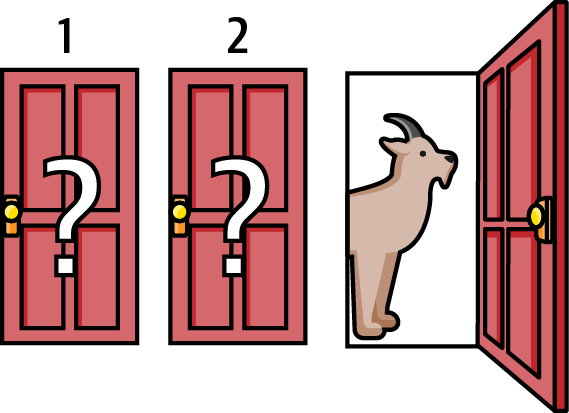
Figure 2-1. The Monty Hall problem1
Now Monty offers you a deal: he gives you the option of sticking with your original choice of door 1 or switching to door 2. Do you switch to door 2 or stay with your original decision of door 1? Try to solve this problem before you read ahead—it will be worth the trouble.
I must admit that when I first came across this problem many years ago, my immediate response was that it doesn’t matter whether you stay or switch doors, since now it is equally likely that the car is behind either door 1 or door 2. So I stayed with my original choice. Turns out that my choice was wrong.
The optimal strategy is to switch doors because, by opening one of the doors, Monty has given you valuable new information which you can use to increase the odds of winning the car. After I worked through the solution and realized I was wrong, I took comfort in the fact that this problem had stumped thousands of PhD statisticians. It had even baffled the great mathematician Paul Erdos, who was only convinced that switching doors was a winning strategy after seeing a simulation of the solution. The in-depth analysis of the Monty Hall problem in this chapter is my “revenge analysis.”
As the following sidebar explains, there may be psychological reasons why people don’t switch doors.
Before we do a simulation of this problem, let’s try to figure out a solution logically by applying the axioms of probability.
Axioms of Probability
Here is a refresher on the axioms, or fundamental rules, of probability. It is simply astonishing that the calculus of probability can be derived entirely from the following three axioms and a few definitions.
Say S is any scenario (also known as an event). In general, we define S as the scenario in which there is a car behind a door. So, S1 is the specific scenario that the car is behind door 1. We define S2 and S3 similarly. The complement of S is S′ (not S) and is the scenario in which there is a goat (not a car) behind the door.
Scenarios S and S′ are said to be mutually exclusive, since there is either a goat or a car, but not both, behind any given door. Since those are the only possible scenarios in this game, S and S′ are also said to be collectively exhaustive scenarios or events. The set of all possible scenarios is called the sample space. Let’s see how we can apply the rules of probability to the Monty Hall game.
- Axiom 1: P(S) ≥ 0
- Probability of an event or scenario, P(S), is always assigned a nonnegative real number. For instance, when Monty shows us that there is no car behind door 3, P(S3) = 0. An event probability of 0 means the event is impossible or didn’t occur.
- Axiom 2: P(S1) + P(S2) + P(S3) = 1
- What this axiom says is that we are absolutely certain that at least one of the scenarios in the sample space will occur. Note that this axiom implies that an event probability of 1 means the event will certainly occur or has already occurred. We know from the rules of the Monty Hall game that there is only one car and it is behind one of the three doors. This means that the scenarios S1, S2, and S3 are mutually exclusive and collectively exhaustive. Therefore, P(S1) + P(S2) + P(S3) = 1. Also note that axioms 1 and 2 ensure that probabilities always have a value between 0 and 1, inclusive. Furthermore, P(S1) + P(not S1) = 1 implies P(S1) = 1 – P(not S1).
- Axiom 3: P(S2 or S3) = P(S2) + P(S3)
- This axiom is known as the sum rule and enables us to compute probabilities of two scenarios that are mutually exclusive. Say we want to know the probability that the car is either behind door 2 or door 3, i.e., we want to know P(S2 or S3). Since the car cannot be behind door 2 and door 3 simultaneously, S2 and S3 are mutually exclusive, i.e., P(S2 and S3) = 0. Therefore, P(S2 or S3) = P(S2) + P(S3).
Probability Distributions Functions
A probability mass function (PMF) provides the probability that a discrete variable will have a particular value, such as those computed in the Monty Hall problem. A PMF only provides discrete and finite values. A cumulative distribution function (CDF) enumerates the probability that a variable is less than or equal to a particular value. The values of a CDF are always non-decreasing and between 0 and 1 inclusive.
A probability density function (PDF) provides the probability that a continuous variable will fall within a range of values. A PDF can assume infinitely many continuous values. However, a PDF assigns a zero probability to any specific point estimate. It might seem surprising that a PDF can be greater than 1 at different points in the distribution. That’s because a PDF is the derivative or slope of the (CDF) and has no constraint on its value not exceeding 1.
We will apply the axioms of probability to solve the Monty Hall problem. It is very important to note that in this book, we don’t make the conventional distinction between a deterministic variable and a random variable. This is because we interpret probability as a dynamic, extrinsic property of the information about an event, which may or may not be repeatable or random. The only distinction we make is a commonsensical one between a variable and a constant. Events for which we have complete information are treated as constants. All other events are treated as variables.
For instance, after Monty places a car behind one of the doors and goats behind the other two, there is no randomness associated with what entity lies behind which door. All such events are now static and nonrandom for both Monty and his audience. However, unlike his audience, Monty is certain where the car is placed. For Monty, the probability that the car is behind a specific door is a constant, namely 1 for the door he chose to place the car behind and 0 for the other two doors he chose to place the goats behind. Since we lack any information about the location of the car when the game begins, we can treat it as a variable whose value we can update dynamically based on new information. For us, these events are not deterministic or random. Our probabilities only reflect our lack of information. However, we can apply the calculus of probability theory to estimate and update our estimates of where the car has been placed. So let’s try to figure that out, without further ado.
Since each scenario is mutually exclusive (there is either a goat or a car behind each door) and collectively exhaustive (those are all the possible scenarios), their probabilities must add up to 1, since at least one of the following scenarios must occur:
- P(S1) + P(S2) + P(S3) = 1 (Equation 2.1)
Before we make a choice, the most plausible assumption is that the car is equally likely to be behind any one of the three doors. There is nothing in the rules of the game to make us think otherwise, and Monty Hall hasn’t given us any hints to the contrary. So it is reasonable to assume that P(S1)=P(S2)=P(S3). Using Equation 2.1, we get:
- 3 × P(S1) = 1 or P(S1) = ⅓ (Equation 2.2)
Since P(S1) = P(S2) = P(S3), Equation 2.2 implies that it is logical to assume that there is a ⅓ probability that the car is behind one of the three doors.
By the sum rule, the probability that the car is behind either door 2 or door 3 is:
- P(S2 or S3) = P(S2) + P(S3) = ⅓ + ⅓ = ⅔ (Equation 2.3)
After you choose door 1 and Monty opens door 3, showing you a goat, P(S3) = 0. Substituting this value in Equation 2.3 and solving for P(S2), we get:
- P(S2) = P(S2 or S3) – P(S3) = ⅔ – 0 = ⅔ (Equation 2.4)
So switching your choice from door 1 to door 2 doubles your chances of winning the car: it goes from ⅓ to ⅔. Switching doors is the optimal betting strategy in this game. See Figure 2-2.
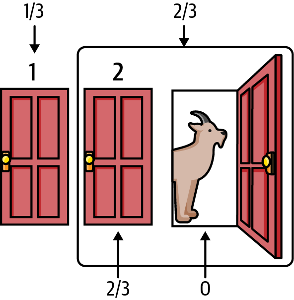
Figure 2-2. A simple logical solution to the Monty Hall problem3
It is important to note that because of uncertainty, there is still a ⅓ chance that you could lose if you switch doors. In general, randomness of results makes it hard and frustrating to determine if your investment or trading strategy is a winning one or a lucky one. It is much easier to determine a winning strategy in the Monty Hall problem because it can be determined analytically or by simulating the game many times, as we will do shortly.
Inverting Probabilities
Let’s develop a more rigorous analytical solution to the Monty Hall problem. To do that, we need to understand conditional probabilities and how to invert them. This is the equivalent of understanding the rules of multiplication and division of ordinary numbers. Recall that when we condition a probability, we revise the plausibility of a scenario or event by incorporating new information from the conditioning data. The conditional probability of a scenario H given a conditioning dataset D is represented as P(H|D), which reads as the probability of H given D and is defined as follows:
- P(H|D) = P(H and D) / P(D) provided P(D) ≠ 0 since division by 0 is undefined
The division by P(D) ensures that probabilities of all scenarios conditioned on D will add up to 1. Recall that if two events are independent, their joint probabilities are the product of their individual probabilities. That is, P(H and D) = P(H) × P(D) if knowledge of D does not improve our probability of H, and vice versa.
The definition of conditional probability of P given H also implies that P(H and D) = P(H|D) × P(D). This is called the product rule. We can now derive the inverse probability rule from the product rule. We know from the symmetry of the joint probability of two events:
P(H and D) = P(D and H)
P(H|D) × P(D) = P(D|H) × P(H)
P(H|D) = P(D|H) × P(H) / P(D)
And that, ladies and gentlemen, is the proof of the famous and wrongly named “Bayes’s theorem.” If only all mathematical proofs were so easy! As you can see, this alleged theorem is a trivial reformulation of the product rule. It’s as much a theorem as multiplying two numbers and solving for one of them in terms of their product (for example, H = H × D/D). The hard part and the insightful bit is interpreting and applying the formula to invert probabilities and solve complex, real-world problems. Since the 1950s, the previously mentioned formula has also been wrongly known as Bayes’s theorem. See the following sidebar.
In this book we will correct this blatant injustice and egregious misnomer by referring to the rule by its original name, the inverse probability rule. This is what the rule was called for over two centuries before R. A. Fisher referred to it pejoratively as Bayes’s rule in the middle of the 20th century. I suspect that by attaching the name of an amateur mathematician to an incontrovertible mathematical rule, Fisher was able to undermine the inverse probability rule so that he could commit the prosecutor’s fallacy with impunity under the pious pretense of only “letting the data speak for themselves.” Fisher’s “worse than useless” statistical inference methodology will be discussed further in Chapter 4. Also, in this book, we revert to the original name of the rule since it has a longer, authenitic tradition, and the alternative of calling the inverse probability rule the Laplace-Bernoulli-Moivre-Bayes-Price rule is way too long.
Furthermore, we will refer to Bayesian statistics as epistemic statistics and Bayesian inference as probabilistic inference. Just as frequentist statistics interprets probability as the relative limiting frequency of an event, epistemic statistics interprets probability as a property of information about an event. Hopefully, this will move us away from wrongly attributing this important scientific endeavor and body of knowledge to one person whose contributions to this effort may be dubious. In fact, there is no evidence to suggest that Bayes was even a Bayesian as the term is used today.
Epistemic statistics in general and the inverse probability rule in particular are the foundation of probabilistic machine learning, and we will discuss it in depth in the second half of this book. For now, let’s apply it to the Monty Hall problem and continue with the same definitions of S1, S2, and S3 and their related probabilities. Now we define our dataset D, which includes two observations: you choose door 1; and based on your choice of door 1, Monty opens door 3 to show you a goat. We want to solve for P(S2|D), i.e., the probability that the car is behind door 2, given dataset D.
We know from the inverse probability rule that this equals P(D|S2) × P(S2)/P(D). The challenging computation is P(D), which is the unconditional or marginal probability of seeing the dataset D regardless of which door the car is behind. The rule of total probability allows us to compute marginal probabilities from conditional probabilities. Specifically, the rule states that the marginal probability of D, P(D), is the weighted average probability of realizing D under different scenarios, with P(S) giving us the specific probabilities or weights for each scenario in the sample space of S:
- P(D) = P(D|S1) × P(S1) + P(D|S2) × P(S2) + P(D|S3) × P(S3)
We have estimated the probabilities of the three scenarios at the beginning of the Monty Hall game, namely P(S1) = P(S2) = P(S3) = ⅓. These are going to be the weights for each possible scenario. Let’s compute the conditional probabilities of observing our dataset D. Note that by P(D|S1) we mean the probability of seeing the dataset D, given that the car is actually behind door 1 and so on.
If the car is behind door 1 and you pick door 1, there are goats behind the other two doors. So Monty can open either door 2 or door 3 to show you a goat. Thus, the probability of Monty opening door 3 to show you a goat, given that you chose door 1, is ½, or P(D|S1) = ½.
If the car is behind door 2 and you have chosen door 1, Monty has no choice but to open door 3 to show you a goat. So P(D|S2) = 1.
If the car is behind door 3, the probability of Monty opening door 3 is zero, since he would ruin the game and you would get the car just for showing up. Therefore, P(D|S3) = 0.
We plug the numbers into the rule of total probability to calculate the marginal or unconditional probability of observing the dataset D in the game:
- P(D) = P(D|S1) × P(S1) + P(D|S2) × P(S2) + P(D|S3) × P(S3)
- P(D) = [½ × ⅓] + [1 × ⅓ ] + [0 × ⅓ ] = ½
Now we have all the probabilities we need to use in the inverse probability rule to calculate the probability that the car is behind door 2, given our dataset D:
- P(S2|D) = P(D|S2) × P(S2) / P(D)
- P(S2|D) = [1 × ⅓ ] / ½ = ⅔
We can similarly compute the probability that the car is behind door 1, given our dataset D:
- P(S1|D) = P(D|S1) × P(S1) / P(D)
- P(S1|D) = [½ × ⅓] / ½ = ⅓
Clearly, we double our chances by switching, since P(S2|D) = 2P(S1|D) = ⅔. Note that there is still a ⅓ chance that you can win by not switching. But like trading and investing, your betting strategy should always put the odds in your favor.
Simulating the Solution
Still not convinced? Let’s solve the Monty Hall problem by using a powerful numerical method called Monte Carlo simulation (MCS), which we mentioned in the previous chapter. This powerful computational method is applied by theoreticians and practitioners in almost every field, including business and finance. Recall that MCS samples randomly from probability distributions to generate numerous probable scenarios of a system whose outcomes are uncertain. It is generally used to quantify the uncertainty of model outputs. The following MCS code shows how switching doors is the optimal betting strategy for this game if played many times:
importrandomimportmatplotlib.pyplotasplt# Number of iterations in the simulationnumber_of_iterations=[10,100,1000,10000]fig,axs=plt.subplots(nrows=2,ncols=2,figsize=(8,6))fori,number_of_iterationsinenumerate(number_of_iterations):# List to store results of all iterationsstay_results=[]switch_results=[]# For loop for collecting resultsforjinrange(number_of_iterations):doors=['door 1','door 2','door 3']# Random selection of door to place the carcar_door=random.choice(doors)# You select a door at randomyour_door=random.choice(doors)# Monty can only select the door that does not have the car and one# that you have not chosenmonty_door=list(set(doors)-set([car_door,your_door]))[0]# The door that Monty does not open and the one you have# not chosen initiallyswitch_door=list(set(doors)-set([monty_door,your_door]))[0]# Result if you stay with your original choice and it has the# car behind itstay_results.append(your_door==car_door)# Result if you switch doors and it has the car behind itswitch_results.append(switch_door==car_door)# Probability of winning the car if you stay with your original# choice of doorprobability_staying=sum(stay_results)/number_of_iterations# Probability of winning the car if you switch doorsprobability_switching=sum(switch_results)/number_of_iterationsax=axs[i//2,i%2]# Plot the probabilities as a bar graphax.bar(['stay','switch'],[probability_staying,probability_switching],color=['blue','green'],alpha=0.7)ax.set_xlabel('Strategy')ax.set_ylabel('Probability of Winning')ax.set_title('After{}Simulations'.format(number_of_iterations))ax.set_ylim([0,1])# Add probability values on the barsax.text(-0.05,probability_staying+0.05,'{:.2f}'.format(probability_staying),ha='left',va='center',fontsize=10)ax.text(0.95,probability_switching+0.05,'{:.2f}'.format(probability_switching),ha='right',va='center',fontsize=10)plt.tight_layout()plt.show()
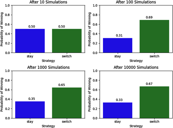
As you can see from the results of the simulations, switching doors is the winning strategy over the long term. The probabilities are approximately the same as in the analytical solution if you play the game ten thousand times. The probabilities become almost exactly the same as the analytical solution if you play the game over a hundred thousand times. We will explore the theoretical reasons for these results in particular, and MCS in general, in the next chapter.
However, it is not clear from the simulation if switching doors is the right strategy in the short term (10 trials), especially if the game is played only once. We know that Monty is not going to invite us back to play the game again regardless of whether we win or lose the car. So can we even talk about probabilities for one-off events? But what do we mean by probabilities anyway? Does everyone agree on what it means? Let’s explore that now.
Meaning of Probability
Two major schools of thought have been sparring over the fundamental meaning of probability—the very soul of statistical inference—for about a century. The two camps disagree on not only the fundamental meaning of probability in those axioms we enumerated, but also the methods for applying the axioms consistently to make inferences. These core differences have led to the development of divergent theories of statistical inference and their implementations in practice.
Frequentist Probability
Statisticians who believe that probability is a natural, immutable property of an event or physical object, and that it is measured empirically as a long-run relative frequency, are called frequentists. Frequentism is the dominant school of the statistics of modern times, in both academic research and industrial applications. It is also known as orthodox, classical, or conventional statistics.
Orthodox statisticians claim that probability is a naturally occurring attribute of an event or physical phenomenon. The probability of an event should be measured empirically by repeating similar experiments ad nauseam—either in reality or hypothetically, using one’s imagination or using computer simulations. For instance, if an experiment is conducted N times and an event E occurs with a frequency of M times, the relative frequency M/N approximates the probability of E. As the number of experimental trials N approaches infinity, the probability of E equals M/N. Figure 2-3 shows a histogram of the long-run relative frequencies of the sum of two fair dice rolled many times.
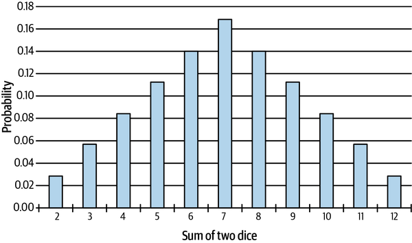
Figure 2-3. Long-run relative frequencies of the sum of two fair dice5
Frequentists consider any alternative interpretation of probability as anathema, almost blasphemous. However, their definition of probability is ideological and not based on scientific experiments. As will be discussed later in the chapter, dice and coins don’t have any static, intrinsic, “true” probabilities. For instance, coin tosses are not random but based on the laws of physics and can be predicted with 100% accuracy using a mechanical coin flipper. These experiments make a mockery of the frequentist definition of probability, which shows an egregious ignorance of basic physics. In Chapter 4, we will examine how the frequentist approach to probability and statistics has had a profoundly damaging impact on the theory and practice of social sciences in general and economic finance in particular, where the majority of the published research using their methods is false.
Epistemic Probability
The other important school of thought is popularly and mistakenly known as Bayesian statistics. As mentioned earlier, this is an egregious misnomer, and in this book we will refer to this interpretation as epistemic probability. Probability has a simpler, more intuitive meaning in the epistemic school: it is an extension of logic and quantifies the degree of plausibility of the event occurring based on the current state of knowledge or ignorance. Epistemic probabilities are dynamic, mental constructs that are a function of information about events that may or may not be random or repeatable.
Probabilities are updated as more information is acquired using the inverse probability rule. Most importantly, the plausibility of an event is expressed as a probability distribution as opposed to a point estimate. This quantifies the degree of plausibility of various outcomes that can occur given the current state of knowledge. Point estimates are avoided as much as possible, given the uncertainties endemic in life and business. Also, recall that the probability of a point estimate is zero for probability density functions. Probabilistic ML is based on this school of thought.
It is important to note that the epistemic interpretation of probability is broad and encompasses the frequentist interpretation of probability as a special limiting case. For instance, in the Monty Hall problem, we assumed that it is equally likely that a car is behind one of three doors; the epistemic and frequentist probabilities are both ⅓. Furthermore, both schools of thought would come to the same conclusion that switching doors doubles your probability and is a winning strategy. However, the epistemic approach did not need any independent and identically distributed trials of the game to estimate the probabilities of the two strategies. Similarly, for simple games of chance such as dice and cards, both schools of probability give you the same results, but frequentists need to imagine resampling the data, or actually conduct simulations.
Over the last century, frequentist ideologues have disparaged and tried to destroy the epistemic school of thought in covert and overt ways. Amongst other things, they labeled epistemic probabilities subjective, which in science is often a pejorative term. All models, especially those in the social and economic sciences, have assumptions that are subjective by definition, as they involve making design choices among many available options.
In finance and investing, subjective probabilities are the norm and are desirable, as they may lead to a competitive advantage. Subjective probabilities prevent the herding and groupthink that occurs when everyone follows the same “objective” inference or prediction about an event. What epistemic statistics will ensure is that our subjective probabilities are coherent and consistent with probability theory. If we are irrational or incoherent about the subjective probabilities underlying our investment strategy, other market participants will exploit these inconsistencies and make a Dutch book of bets against us. This concept is the sports-betting equivalent of a riskless arbitrage opportunity where we lose money on our trades or investments to other market participants no matter what the outcomes are.
The frequentist theory of statistics has been sold to academia and industry as a scientifically rigorous, efficient, robust, and objective school of thought. Nothing could be further from the truth. Frequentists use the maximum likelihood estimation (MLE) method to learn the optimal values of their model parameters. In their fervor to “only let the data speak” and make their inferences bias-free, they don’t explicitly apply any prior knowledge or base rates to their inferences. They then claim that they have bias-free algorithms that are optimal for any class of problems. But the NFL theorems clearly state that this is an impossibility.
The NFL theorems prove mathematically that the claim that an algorithm is both bias-free and optimal for all problem domains is false. That’s a free lunch, and not allowed in ML, search, and optimization. If an algorithm is actually bias-free as claimed, the NFL theorems tell us that it will not be optimal for all problem domains. It will have high variance on different datasets, and its performance will be no better than random guessing when averaged across all target distributions. The risk is that it will be worse than random guessing, which is what has occurred in the social and economic sciences, where the majority of research findings are false (see Chapter 4 for references). If the frequentist’s defense is that all target distributions are not equally likely in this world, they need to realize that any selection of a subset of target distributions is a foolish admission of bias, because that involves making a subjective choice.
But we don’t even have to use the sophisticated mathematics and logic of the NFL theorems to expose the deep flaws of the frequentist framework. In Chapter 4, we will examine why frequentist inference methods are “worse than useless,” because they violate the rules of multiplication and division of probabilities (the product and inverse probability rules) and use the statistical skullduggery of the prosecutor’s fallacy in their hypothesis testing methodology.
Despite the vigorous efforts of frequentists, epistemic statistics has been proven to be theoretically sound and experimentally verified. As a matter of fact, it is actually the frequentist version of probability that fails miserably, exposing its frailties and ad hoceries when subjected to complex statistical phenomena. For instance, the frequentist approach cannot be logically applied to image processing and reconstruction, where the sampling distribution of any measurement is always constant. Probabilistic algorithms dominate the field of image processing, leveraging their broader, epistemic foundation.6
A summary of the differences between the frequentist and epistemic statistics have been outlined in Table 2-1. Each of the differences have been or will be explained in this book and supported by plenty of scholarly references.
| Dimension | Frequentist statistics | Epistemic statistics |
|---|---|---|
| Probability | An intrinsic, static property of the long-run relative frequency of an event or object. Not supported by physics experiments. | A dynamic, extrinsic property of the information about any event, which may or may not be repeatable or random. |
| Data | Sources of variance that are treated as random variables. Inferences don’t work on small datasets. | Known and treated as constants. Size of the dataset is irrelevant. |
| Parameters | Treated as unknown or unknowable constants. | Treated as unknown variables. |
| Models | There is one “true” model with optimal parameters that explain the data. | There are many explanatory models with varying plausibilities. |
| Model types | Discriminative models—only learn a decision boundary. Cannot generate new data. | Generative models—learn the underlying structure of the data. Simulates new data. |
| Model assumptions | Implicit in null hypotheses, significance levels, regularizations, and asymptotic limits. | Most important model assumptions are explicitly stated and quantified as prior probabilities. |
| Inference method | Maximum likelihood estimation. | Inverse probability rule / product rule. |
| Hypothesis testing | Null hypothesis significance testing is binary and is guilty of the prosecutor’s fallacy. | Degrees of plausibility assigned to many different hypotheses. |
| Uncertainty types | Only deals with aleatory uncertainty. | Deals with aleatory and epistemic uncertainties. |
| Uncertainty quantification | Confidence intervals are epistemologically incoherent and mathematically flawed. P-values are guilty of the inverse fallacy. | Credible intervals based on logic and common sense. Epistemologically coherent and mathematically sound. |
| Computational complexity | Low. | Medium to high. |
| No free lunch (NFL) theorems | Violates the NFL theorems. Doesn’t include prior knowledge, so algorithms have high variance. When averaged across all possible problems, their performance is no better than random guessing. | Consistent with NFL theorems. Prior knowledge lowers the variance of algorithms, making them optimal for specific problem domains. |
| Scientific methodology | Ideological, unscientific, ad hoc methods under a facade of objectivity. Denies the validity of the inverse probability rule / product rule. Main cause of false findings in social and economic sciences. | Logical and scientific view that systematically integrates prior knowledge based on the inverse probability rule / product rule. Explicitly states and quantifies all objective and subjective assumptions. |
Relative Probability
Are there any objective probabilities in the Monty Hall problem? The car is behind door 2, so isn’t the “true” and objective probability of S2 = 1 a constant? Yes, any host in the same position as Monty will assign S2 = 1, just as any participant would assign S2 = ⅓. However, there is no static, immutable, “true” probability of any event in the sense that it has an ontological existence in this game independent of the actions of humans. If Monty has the car placed behind door 1, S2 = 0 for him but remains constant at ⅓ for any participant.
Probabilities depend on the model used, the phase of the game, and the information available to the participant or the host. As noted previously, probabilities for any participant or host are not subjective but a function of the information they have, since any host and any reasonable participant would arrive at the same probabilities using basic probability theory or common sense. Probability is a mental construct used to quantify uncertainties dynamically.
It is analogous to the physics of special relativity, which have been experimentally verified since Albert Einstein published his monumental paper in 1905. The principle of relativity states that the laws of physics are invariant across all frames of reference that are not accelerating relative to one another. Two observers sharing the same frame of reference will always agree on fundamental measurements of mass, length, and time. However, they will have different measurements of these quantities depending on how their frames of reference are moving relative to one another and compared to the speed of light. The principle of relativity has many important implications, including the fact that there is no such thing as absolute motion. Motion is always relative to a frame of reference.
Figure 2-4 shows two frames of reference, with the primed coordinate system moving at a constant velocity relative to the unprimed coordinate system. Observers O and O′ will agree that the same laws of physics apply in their worlds. However, observers O will claim that they are stationary and that observers O′ are moving forward along the x-axis at a constant velocity (+v). But observers O′ will claim that they are stationary and it is observers O that are moving backward along the x'-axis at a constant velocity (–v). This means that there is no way to say definitively whether O or O′ is really moving. They are both moving relative to each other, but neither one is moving in an absolute sense.
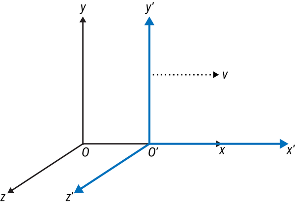
Figure 2-4. The principle of relativity using two frames of reference moving at a constant velocity relative to each other7
I find it useful to think in terms of relative probabilities based on an observer’s frame of reference or access to information as opposed to objective or subjective probabilities. Regardless, probability theory works in all frames of reference we are concerned with. We need it to quantify the profound uncertainties that we have to deal with in our daily personal and professional lives. But before we quantify uncertainty, we need to understand it in some depth.
Risk Versus Uncertainty: A Useless Distinction
In conventional statistics and economics literature, a vacuous distinction is generally made between risk and uncertainty. Supposedly, risk can only be estimated for events that are known and have objective probability distributions and parameters associated with them. Probabilities and payoffs can be estimated accurately, and risk is computed using various metrics. When there are no objective probability distributions or if events are unknown or unknowable, the event is described as uncertain and the claim is made that risks cannot be estimated.
In finance and investing, we are not dealing with simple games of chance, such as casino games, where the players, rules, and probability distributions are fixed and known. Both product and financial markets are quite different from such simple games of chance, where event risks can be estimated accurately. As was discussed in the previous chapter, unknown market participants may use different probability distributions in their models based on their own strategies and assumptions. Even for popular, consensus statistical distributions, there is no agreement about parameter estimates. Furthermore, because markets are not stationary ergodic, these probability distributions and their parameters are continually changing, sometimes abruptly, making a mockery of everyone’s estimates and predictions.
So, based on the conventional definition of risk and uncertainty, almost all investing and finance is uncertain. In practice, this is a useless distinction and stems from useless frequentist statistics and neoclassical economics ideologies about objective, academic models, not from the realities of market participants. As practitioners, we develop our own subjective models based on our experience, expertise, institutional knowledge, and judgment. As a matter of fact, we protect our proprietary, subjective models assiduously, since sharing them with the public would undermine our competitive advantages.
Edward Thorp, the greatest quantitative gambler and trader of all time, invented an options pricing model much before Fischer Black and Myron Scholes published their famous “objective” model in 1973. Since Thorp’s model was a trade secret of his hedge fund, he owed it to his investors not to share his model with the general public and fritter away his company’s competitive advantage. Thorp applied his subjective, numerical, proprietary options model to generate one of the best risk-adjusted returns in history. Black and Scholes applied their “objective,” analytical options pricing model to real markets only to experience near financial ruin and make a hasty retreat to the refuge of the ivory towers of academia.8
Options market makers and derivatives traders like me generally modify the “objective” Black-Scholes pricing model in different ways to correct for its many deep flaws. In doing so, we make our options trading models subjective and proprietary. Most importantly, we make it useful for successfully trading these complex markets.
The real value of the “objective” Black-Scholes options pricing model is clearly not in its accurate pricing of options. It’s common knowledge among academics and practitioners alike that it’s not accurate, especially since it erroneously treats volatility of the underlying asset as a constant. A classic joke about the Black-Scholes model is that you have to put “the wrong number in the wrong formula to get the right price.”
The real value-add of the Black-Scholes model, explaining its enduring popularity among practitioners, is in its enabling communication among market participants who are generally using their own disparate, proprietary options pricing models. It is ironic that despite the Black-Scholes model’s fictitious assumptions and market fantasies, it has contributed significantly to the rapid growth of real-world options markets. Humans are suckers for good works of fiction in any format. Perhaps Black and Scholes should have been awarded a real Nobel Prize in literature.
In epistemic statistics, probabilities are an extension of logic and can be assigned to any uncertain event—known, unknown, and unknowable. We do this by rejecting point estimates and setting the bar extremely high for assuming any event to be a certainty (probability = 1) or an impossibility (probability = 0). That’s why in epistemic statistics we deal only with probability distributions. Unknowable events are acknowledged by using fat-tailed probability distributions like the Cauchy distribution, which has no defined mean or variance, reflecting the fact that almost anything is possible during the holding periods of our trades and investments.
Probability estimates are based on our prior knowledge, observed data, and expertise in making such estimates. But most importantly, they depend on human judgment, common sense, and an understanding of causation, which AI systems are incapable of processing. The degree of confidence we have in our estimates and forecasts will vary depending on many factors, including the nature of the event, the sources of uncertainty, our resources, and our abilities to perform such tasks.
In finance and investing, we don’t have the luxury of not undertaking such imperfect, messy statistical endeavors. We do it knowing full well that these difficult exercises are rife with approximations, riddled with potential errors, and susceptible to the ravages and ridicule of markets. Dwight Eisenhower, former US general and president, explained the value of such exercises when he said, “In preparing for battle I have always found that plans are useless, but planning is indispensable.”9 The alternative of forsaking such statistical exercises by taking comfort in some useless definition of risk and uncertainty is even worse. The worst course of action is to be lulled into a false sense of security by some economic ideology of objective statistical models or normative theory of human behavior and rationality that have no basis in data and the experienced realities of the world.
We reject such useless distinctions between risk and uncertainty. All uncertain events are logically and realistically plausible based on an appropriate probability distribution and boundary conditions. We know that all models are wrong, including the useful ones, and do not pledge any fealty to these shadows of reality.
The Trinity of Uncertainty
Uncertainty is generally classified into three types based on the source from which it arises: aleatory, epistemic, and ontological. These are complex concepts that philosophers and scientists worldwide have endeavored to understand and apply for millennia. Let’s see how we can use the Monty Hall problem to understand the complexities of this trinity of uncertainty. Later, we apply each type of uncertainty to various aspects of machine learning that we are faced with in practice.
Aleatory Uncertainty
Aleatory means “of dice” in Latin. Fundamentally, aleatory uncertainty is the irreducible randomness of outcomes. Both the analytical and simulated solutions to the Monty Hall problem demonstrated that your strategy of staying or switching doors in this game does not guarantee you a win during a single play, or even multiple plays, of the game. You could stay with your original choice of door 1 and have a ⅓ chance of winning the car. You could switch to door 2 and have a ⅓ chance of losing the car. Whenever you play the game, you are indeed rolling the proverbial dice, since the outcome is uncertain.
Actually, it’s more uncertain than rolling dice or tossing a coin, since they both have no aleatory uncertainty, only epistemic uncertainty, as explained in the next section. Tossing a coin is a canonical example of aleatory uncertainty in the current literature on probability and statistics. However, this shows an inexcusable ignorance of the laws of classical physics. It has been experimentally verified that if you know the initial conditions and other parameters of a coin toss, you can predict its outcome with 100% accuracy. That’s because coin tossing is physics, not randomness.10
Statistician and former magician Persi Diaconis had engineers build him a mechanical coin flipper so that he could experiment and study coin tossing. Indeed, he and his colleagues verified that there is no randomness in a coin toss with the mechanical coin flipper.11 The randomness of a coin toss arises from the inconsistency of initial conditions of human coin flipping and from the coin rolling on the ground.
The uncertainty we observe stems from our lack of precise information or knowledge of the physics of the tosses. It is a bad example of aleatory uncertainty. It also demonstrates that coins don’t have any intrinsic, immutable, limiting frequency, as frequentists will have us believe. You can use the physics of the coin toss to make a biased coin honest and vice versa with some practice.12
Tossing coins and rolling dice are examples of epistemic uncertainty, which we will discuss in the next subsection. In contrast to coins or dice, no amount of information about the physical characteristics of the doors or their motion will reduce the aleatory uncertainty of where the car is in the Monty Hall problem. It is a great example of aleatory uncertainty, and why social systems are fundamentally different and much harder to predict than physical systems.
In machine learning (ML), aleatory uncertainty is the source of irreducible error and is generated because of data. It sets the lower bound on the generalization error that can be achieved by any ML model. This endemic noise is generated in two distinct ways:
- Measurement uncertainty
- It is not always possible to measure data with complete accuracy. For instance, when there is high market volatility due to an event, such as the release of an economic report, it is almost impossible to capture every transaction or tick in real time, leading to missing or delayed tick data. Similarly, data transmission errors can lead to missing or corrupt tick data.
- Sampling uncertainty
- Every time we take a random data sample from across a population at a particular time, or sample a stochastic process at different times, the sample statistics, such as mean and variance, will vary from sample to sample. This type of aleatory uncertainty is due to the inherent randomness of the sampling process itself and the variability of the underlying statistical distribution. For example, consumer sentiment surveys taken by different companies result in different statistical estimates. Also, the variance of a stock’s price returns also changes over time. Figure 2-5 shows how a specific random data sample is taken from the population to estimate the population mean and variance.
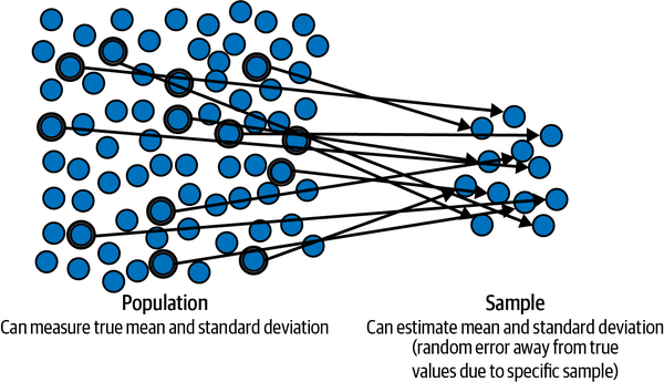
Figure 2-5. Sampling uncertainty because a random sample is drawn to estimate the statistical properties of its population13
Epistemic Uncertainty
Episteme means “knowledge” in Greek. The epistemic uncertainty of any scenario depends on the state of knowledge or ignorance of the person confronting it. Unlike aleatory uncertainty, you can reduce epistemic uncertainty by acquiring more knowledge and understanding. When Monty opens a door to show you a goat, he is providing you with very valuable new information that reduces your epistemic uncertainty. Based on this information from Monty’s response to your choice, the probability of door 1 having a car behind it remained unchanged at ⅓, but the probability for door 2 changed from ⅓ to ⅔, and the probability for door 3 changed from ⅓ to 0.
However, there is no uncertainty for Monty regarding which door the car is behind: his probability for each door is either 1 or 0 at all times. He is only uncertain about which door you are going to pick. Also, once you pick any door, he is certain what he is going to do next. But he is uncertain what you will do when offered the deal. Will you stay with your original choice of door 1 or switch to door 2, and most likely win the car? Monty’s uncertainties are not epistemic but ontological, a fundamentally different nature of uncertainty, which we will discuss in the next subsection.
So we can see from this game that the uncertainty of picking the right door for you is a function of one’s state of knowledge or “episteme.” It is important to note that this is not a subjective belief but a function of information or lack of it. Any participant and any host would have the same uncertainties calculated earlier in this chapter, and switching doors would still be the winning strategy.
Note
This game is also an example of the asymmetry of information that characterizes financial deals and markets. Generally speaking, parties to a deal always have access to differing amounts of information about various aspects of a deal or asset, which leads to uncertainty in their price estimates and deal outcomes. Different information processing capabilities and speeds further exacerbate those uncertainties.
There are many sources of epistemic uncertainty in ML arising from a lack of access to knowledge and understanding of the underlying phenomenon.
They can be categorized in the following ways:- Data uncertainty
- To make valid inferences, we want our data sample to represent the underlying population or data-generating process. For instance, auditors sample a subset of a company’s transactions or financial records during a particular time period to check for compliance with accounting standards. The auditor may fail to detect errors or fraud if the sample is unrepresentative of the population of transactions.
- Model uncertainty
- There is always uncertainty about which model to choose to make inferences and predictions. For example, when making financial forecasts, should we use linear regression or nonlinear regression models? Or a neural network? Or some other model?
- Feature uncertainty
- Assume we pick a linear model as our first approximation and baseline model for financial forecasting. What features are we going to select to make our inferences and forecasts? Why did we select those features and leave out others? How many are required?
- Algorithmic uncertainty
- Now that we have selected features for our linear model, what linear algorithm should we use to train the model and learn its parameters? Will it be ridge regression, lasso regression, support vector machines, or a probabilistic linear regression algorithm?
- Parameter uncertainty
- Say we decide to use a market model and a probabilistic linear regression algorithm as our baseline model. What probability distributions are we going to assign each parameter? Or are the parameters going to be point estimates? What about the hyperparameters—that is, parameters of the probability distributions of parameters? Are they going to be probability distributions or point estimates?
- Method uncertainty
- What numerical method are we going to use in our model to learn its parameters from in-sample data? Will we use the Markov chain Monte Carlo (MCMC) method or variational inference? A Metropolis sampling method or Hamiltonian Monte Carlo sampling method? What values are we going to use for the parameters of the chosen numerical methods? How do we justify those parameter values?
- Implementation uncertainty
- Assume we decide on using the MCMC method. Which software should we use to implement it? PyMC, Pyro, TensorFlow Probability, or Stan? Or are we going to build everything from scratch using Python? What about R or C++?
As the previous discussion shows, designing ML models involves making choices about the objective function, data sample, model, algorithm, and computational resources, among many others. As was mentioned in the previous chapter, our goal is to train our ML system so that it minimizes out-of-sample generalization errors that are reducible.
If we have prior knowledge about the problem domain, we might develop a simple system with few parameters because of such knowledge and assumptions. This is referred to as bias in ML. The risk is that our prior assumptions of the model may be erroneous, leading it to underfit the training data systematically and learn no new patterns or signals from it. Consequently, the model is exposed to bias errors and performs poorly on unseen test data. On the other hand, if we don’t have prior knowledge about the problem domain, we might build a complex model with many parameters to adapt and learn as much as possible from the training data. The risk there is that the model overfits the training data and learns the spurious correlations (noise) as well. This result is that the model introduces errors in its predictions and inferences due to minor variations in the data. These errors are referred to as variance errors and the model performs poorly on unseen test data. Figure 2-6 shows the bias-variance trade-off that needs to made in developing models that minimize reducible generalization errors. This trade-off is made more difficult and dynamic when the underlying data distributions are not stationary ergodic, as they are in finance and investing problems.
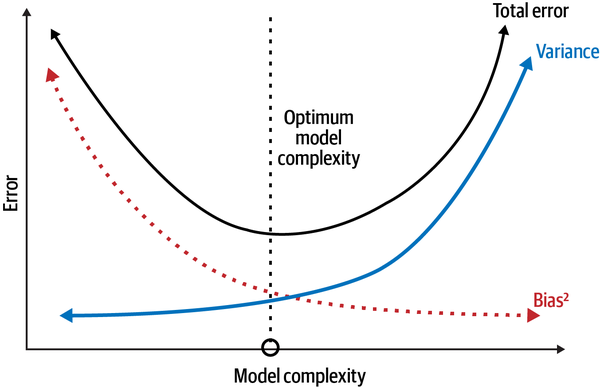
Figure 2-6. The bias-variance trade-off that needs to be made when developing ML models14
Ontological Uncertainty
Ontology is the philosophical study of the nature of being and reality. Ontological uncertainty generally arises from the future of human affairs being essentially unknowable.15
To make the Monty Hall game resemble a real-world business deal or a trade, we have to dive deeper into the objective of the game, namely winning the car. From Monty’s perspective, winning means keeping the car so he can reduce the costs of the show while still attracting a large audience. When the game is viewed in this way, Monty’s knowledge of the car’s placement behind any one of the doors does not decrease his ontological uncertainty about winning the game. This is because he doesn’t know which door you’re going to pick and whether you will stay or switch doors when given the choice to do so. Since his probabilities are the complement of your probabilities, he has a ⅔ chance of keeping the car if you don’t switch doors and ⅓ chance of losing the car to you if you do switch doors.
There are other possible ontological uncertainties for you. Say you show up to play the game a second time armed with the analysis of the game and the door-switching strategy. Monty surprises you by changing the rules and does not open another door to show you a goat. Instead he asks you to observe his body language and tone of voice for clues to help you make your decision. However, Monty has no intention of giving you any helpful clues and wants to reduce your probability of winning to ⅓ regardless of your decision to stay or switch doors. Monty does this because earlier in the week his producer had threatened to cancel the show, since its ratings were falling and it was not making enough money to cover Monty’s hefty salary.
Unexpected changes in business and financial markets are the rule, not the exception. Markets don’t send out a memo to participants when undergoing structural changes. Companies, deals, and trading strategies fail regularly and spectacularly because of these types of changes. It is similar to the way one of Hemingway’s characters described how he went bankrupt: “Two ways…Gradually and then suddenly.”16
In ML, ontological uncertainty occurs when there is a structural discontinuity in the underlying population or data-generating process, as was discussed in Chapter 1, where we had to change the model from a binomial to a trinomial one. In finance and investing, the source of ontological uncertainty is the complexity of human activities, such as political elections, monetary and fiscal policy changes, company bankruptcies, and technological breakthroughs, to name just a few. Only humans can understand causality underlying these changes and use common sense to redesign the ML models from scratch to adapt to a new regime. Figure 2-7 shows the types of intelligent systems that are used in practice to navigate aleatory, epistemic, and ontological uncertainties of finance and investing.
As you can see, designing models involves understanding different types of uncertainties, with each entailing a decision among various design options. Answers to these questions require prior knowledge of the problem domain and experience experimenting with many different models and algorithms. They cannot be derived from first principles of deductive logic or learned only from sample data that are not stationary ergodic. This seems obvious to practitioners like me. What might surprise most practitioners, as it did me, is that there is a set of mathematical theorems called the no free lunch (NFL) theorems that prove the validity of our various approaches.
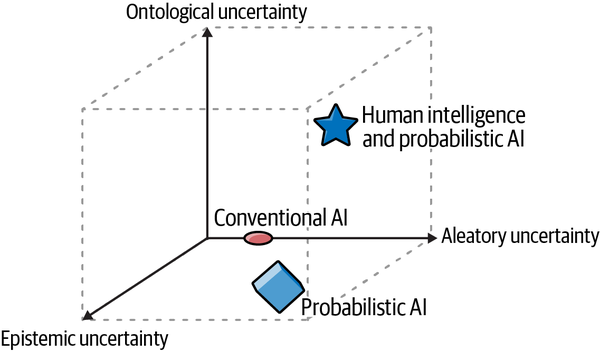
Figure 2-7. Human intelligence supported by probabilistic AI systems is the most useful model for navigating the three-dimensional uncertainties of finance and investing
The No Free Lunch Theorems
In 1891, Rudyard Kipling, a Nobel laureate in literature and an English imperialist from the province of Bombay, recounted a visit to a saloon in his travel journal American Notes: “It was the institution of the ‘free lunch’ that I had struck. You paid for a drink and got as much as you wanted to eat. For something less than a rupee a day a man can feed himself sumptuously in San Francisco, even though he be a bankrupt. Remember this if ever you are stranded in these parts.”17
Fortuitously, I have been “stranded” in these parts for some time now and have a few rupees left over from my recent visit to the former province of Bombay. Unfortunately, this once popular American tradition of the “free lunch” is no longer common and has certainly disappeared from the bars in San Francisco, where a couple of hundred rupees might get you some peanuts and a glass of tap water. However, the idea that lunch is never free and we eventually pay for it with a drink—or personal data, or something else—has persisted and is commonly applied in many disciplines, especially economics, finance, and investing.
David Wolpert, an eminent computer scientist and physicist, discovered that this idea also applied to machine learning and statistical inference. In 1996 he shocked both these communities by publishing a paper that proved mathematically the impossibility of the existence of a superior ML learning algorithm that can solve all problems optimally. Prior knowledge of the problem domain is required to select the appropriate learning algorithm and improve its performance.18 Wolpert, who was a postdoctoral student at the time of the publication, was subjected to ad hominem attacks by industry executives and derision by academics who felt threatened by these theorems because they were debunking their specious claims of discovering such optimal, bias-free, general purpose ML learning algorithms.
Wolpert subsequently published another paper with William Macready in 1997 that provided a similar proof for search and optimization algorithms.19 These theorems are collectively known as the no free lunch (NFL) theorems.Please note that prior knowledge and assumptions about the problem domain that is used in the selection and design of the learning algorithm is also referred to as bias. Furthermore, a problem is defined by a data generating target distribution that the algorithm is trying to learn from training data. A cost function is used to measure the performance of the learning algorithm on out-of-sample test data. These theorems have many important implications for ML that are critical for us to understand.
One important implication is that the performance of all learning algorithms when averaged across all problem domains will be the same. As shown in Figure 2-8, each data scientist has a different learning algorithm (A, B, C) whose performance is measured on unseen data of four different problem domains (apples, pears, tools, and shoes). On the apple problem domain, all three learning algorithms perform optimally. So we don’t have a unique optimal learning algorithm for the apple domain or any other problem domain for that matter. However, the learning algorithms have varying performance measures on each of the other three problem domains. None of the learning algorithms performs optimally on all four problem domains. Regardless, the performance of all three learning algorithms when considered independently and averaged across the four problem domains is the same at 32 / 4 = 8.
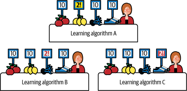
Figure 2-8. The performance of all three learning algorithms averaged across all four problem domains is the same, with a score of 8.20
This example illustrates the central idea in the NFL theorems that there are no mathematical reasons to prefer one learning algorithm over another based on expected performance across all problem domains. Since learning algorithms have varying performances on different problem domains, we must use our empirical knowledge of a specific problem domain to select a learning algorithm that is best aligned with the domain’s target function. So how well the learning algorithm performs is contingent on the validity of our domain knowledge and assumptions. There are no free lunches in ML.
If we don’t make the payment of prior knowledge to align our learning algorithm with the underlying target function of the problem domain, like the freeloading frequentists claim we must do to remain unbiased, the learning algorithm’s predictions based on unseen data will be no better than random guessing when averaged over all possible target distributions. In fact, the risk is that it might be worse than random guessing. So we can’t have our lunch and not pay for it in ML. If we bolt for the exit without paying for our lunch, we’ll realize later that what we wolfed down was junk food and not a real meal.
The most common criticism of NFL theorems is that all target distributions are not equally likely in the real world. This criticism is spurious and misses the point of using such a mathematical technique. The reason is that in the bias-free world that frequentists fantasize about, we are required to assign equal probability to all possible target distributions by definition. Any selection of a single target distribution from a finite set of all possible target distributions must necessarily involve making a subjective choice, which, by definition of an unbiased world, is not allowed. Because we are forbidden in a bias-free world from using our prior knowledge of the problem domain to pick a single target distribution, the performance of an unbiased algorithm must be averaged over all possible, equally likely target distributions. The result is that the unbiased algorithm’s average performance on unseen data is reduced to being no better than random guessing. The frequentist trick of implicitly selecting a target function while obfuscating their biased choice with statistical jargon and a sham ideology of objectivity doesn’t stand up to scrutiny.
The most important practical implication of the NFL theorems is that good generalization performance of any learning algorithm is always context and usage dependent. If we have sound prior knowledge and valid assumptions about our problem domain, we should use it to select and align the learning algorithm with the underlying structure of our specific problem and the nature of its target function. While this may introduce biases into the learning algorithm, it is a payment worth making, as it will lead to better performance on our specific problem domain.
But remember that this optimality of performance is because of our “payment” of prior knowledge. Since our learning algorithm will be biased toward our problem domain, we should expect that it will almost surely perform poorly on other problem domains that have divergent underlying target functions, such that its average performance across all problem domains will be no better than the performance of another learning algorithm.
But the performance of our learning algorithms on other problem domains is not our concern. We are not touting our biased learning algorithms and models as a panacea for all problem domains. That would be a violation of the NFL theorems. In this book, we are concerned primarily with optimizing our probabilistic machine learning algorithms and models for finance and investing.
Most importantly, the NFL theorems are yet another mathematical proof of the sham objectivity and deeply flawed foundations of frequentist/conventional statistics. The frequentists’ pious pretense of not using prior domain knowledge explicitly and making statistical inferences based solely on in-sample data is simply wrong and has had serious consequences for all the social sciences. It has led to base rate fallacies and a proliferation of junk studies whose results are no better than random guessing. We will discuss this further in Chapter 4.
Investing and the Problem of Induction
Inductive reasoning synthesizes information from past observations to formulate general hypotheses that will continue to be plausible in the future. Simply put, induction makes inferences about the general population distribution based on an analysis of a random data sample. Figure 2-9 shows how deductive and inductive reasoning are used in the scientific method.
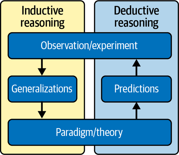
Figure 2-9. The use of inductive and deductive reasoning in the scientific method21
This is generally what we do in finance and investing. We analyze past data to detect patterns (such as trends) or formulate causal relationships between variables (such as earnings and price returns) or human behavior (such as fear and greed). We try to come up with a cogent thesis as to why these historical patterns and causal relationships will most likely persist in the future. Such financial analysis is generally divided into two types:
- Technical analysis
This is the study of historical patterns of an asset’s price and volume data during any time period based on its market dynamics of supply and demand. Patterns and statistical indicators are correlated with the asset’s future uptrends, downtrends, or trendless (sideways) price movements. See Figure 2-10 for a technical pattern called a double bottom, which is a signal that indicates the asset will rally in the future after it is confirmed that it has found support at the second bottom price.
Generally speaking, technical analysts are not concerned with the nature of the asset or what is causing its prices to change at any given time. This is because all necessary information is assumed to be reflected in the price and volume data of the asset. Technical analysts are only concerned with detecting patterns in historical prices and volumes, computing statistical indicators, and using their correlations to predict future price changes of the asset. Technical investing and trading strategies assume that historical price and volume patterns and their related price correlations will repeat in the future because human behavior and the market dynamics of supply and demand on which they are based don’t essentially change.
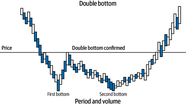
Figure 2-10. A double bottom technical pattern predicts that the price of the asset will rise in the future.
- Fundamental analysis
- This is the study of financial, economic, and human behavior. Analysts study historical company financial statements and economic, industry, and consumer reports. Using past empirical data, statistical analysis, or academic financial theories, analysts formulate causal mechanisms between features (or risk factors) and the fundamental value of an asset. Fundamental analysts are mainly concerned with the nature of the asset that they analyze and the underlying causal mechanisms that determine its valuation.
For instance, the discounted cash flow (DCF) model is used extensively for valuing assets, such as the equity and debt of a company or the value of its factory. Fundamental analysts forecast the cash flows that a company or capital project is expected to generate in the future (typically three to five years) and discount them back to the present using an interest rate to account for the opportunity cost of the company’s capital. They also forecast macroeconomic variables like tax rates, inflation rates, gross domestic product, and currency exchange rates, among others. The fundamental principle of the DCF model is that cash tomorrow is worth less than cash today and must be discounted accordingly. This assumes that interest rates are always positive and cash can be lent out to earn interest at the appropriate rate. By forgoing the opportunity to lend out their cash at the appropriate rate, an investor incurs an opportunity cost that is reflected in the discount rate. See Figure 2-11.
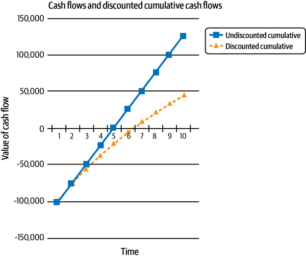
Figure 2-11. Cash flows need to be discounted because cash tomorrow is worth less than cash today, assuming interest rates are positive
The DCF model is very sensitive to minor changes in the discount rate and the projected growth rate of its cash flows. This is why the interest rate set by central bankers is pivotal to the valuation of all assets, as it directly impacts an investor’s cost of capital. Fundamental trading and investing strategies assume that the formulated causal mechanisms between features (risk factors) and asset valuation will persist into the future.
All other methods, such as quantitative analysis or machine learning, use some combination of technical and fundamental analysis. Regardless, how do we know that the patterns of technical analysis and causal relationships of fundamental analysis that have been observed thus far will continue to persist in the future? Well, because the past has resembled the future so far. But that is exactly what we are trying to prove in the first place! This circular reasoning is generally referred to as the problem of induction.
This is a confounding metaphysical problem that has been investigated by the Carvaka school of Indian philosophy, at least 2,400 years before David Hume articulated the problem in the 18th century for a Western audience.22 We can ignore the problem of induction in physics (see Sidebar). However, we cannot do that in the social sciences, especially finance and investing, where it is a clear and present danger to any extrapolation of the past into the future. That’s because human beings have free will, emotions, and creativity, and they react to one another’s actions in unpredictable ways. Sometimes history repeats itself, sometimes it rhymes, and sometimes it makes no sense at all. That’s why Securities and Exchange Commission (SEC) in the United States mandates all marketing materials in the investment management industry to have a disclaimer that states past returns are no guarantee of future results. This trite but true statement is merely echoing the age-old problem of induction. Unlike the physical universe, social systems don’t need infinite time and space to generate seemingly impossible events. An average lifetime is more than enough to witness a few of these mind-boggling events. For instance, in the last decade, over 15 trillion dollars’ worth of bonds were issued with negative interest rates in Japan and Europe! Negative interest rates contradict common sense, fundamental principles of finance, and the foundation of the DCF model.
The Problem of Induction, NFL Theorems, and Probabilistic Machine Learning
Inductive inference is foundational to ML All ML models are built on the assumption that patterns discovered in past training data will persist in future unseen data. It is important to note that the NFL theorems are a brilliant algorithmic restatement of the problem of induction within a probabilistic framework. In both frameworks, we have to use prior knowledge or assumptions about the problem domain to make predictions that are better than chance on unseen data. More importantly, this knowledge cannot be acquired from in-sample data alone or from principles of deductive logic or theorems of mathematics. Prior knowledge based on past empirical observations and assumptions about the underlying structural unity of the observed phenomenon or data-generating target function are required. It is only when we apply our prior knowledge about a problem domain can we expect to optimize our learning algorithm for making predictions on unseen data that will be much better than random guessing.
Most importantly, epistemic statistics embraces the problem of induction zealously and directly answers its central question: can we ever be sure that the knowledge that we have acquired from past observations is valid and will continue to be valid in the future? Of course not—the resounding answer is, we can almost never be sure. Learning continually from uncertain and incomplete information is the foundation on which epistemic statistics and probabilistic inference is built.
Consequently, as we will see in Chapter 5, epistemic statistics provides a probabilistic framework for machine learning that systematically integrates prior knowledge and keeps updating it with new observations because we can never be certain that the validity of our knowledge will continue to persist into the future. Almost all knowledge is uncertain to a greater or lesser degree and is best represented as a probability distribution, not a point estimate. Forecasts about the future (predictions) and the past (retrodictions) are also generated from these models as predictive probability distributions. Its biggest challenge, however, is dealing with ontological uncertainty, for which human intelligence is crucial.
Summary
In this chapter, we used the famous Monty Hall problem to review the fundamental rules of probability theory and apply them to solve the Monty Hall problem. We also realized how embarassingly easy it is to derive the inverse probability rule that is pivotal to epistemic statistics and probabilistic machine learning. Furthermore, we used the Monty Hall game to explore the profound complexities of aleatory, epistemic, and ontological uncertainty that pervade our lives and businesses. A better understanding of the three types of uncertainty and the meaning of probability will enable us to analyze and develop appropriate models for our probabilistic ML systems to solve the difficult problems we face in finance and investing.
We know for a fact that even a physical object like a coin has no intrinsic probability based on long-term frequencies. It depends on initial conditions and the physics of the toss. Probabilities are epistemic, not ontological—they are a map, not the terrain. It’s about time frequentists stop fooling themselves and others with their mind-projection fallacies and give up their pious pretense of objectivity and scientific rigor.
The NFL theorems can be interpreted as restating the problem of induction for machine learning in general and finance and investing in particular. Past performance of an algorithm or investment strategy is no guarantee of its future performance. The target distribution of the problem domain or the out-of-sample dataset may change enough to degrade the performance of the algorithm and investment strategy. In other words, it is impossible to have a unique learning algorithm or investment strategy that is both bias-free and optimal for all problem domains or market environments. If we want an optimal algorithm for our specific problem domain, we have to pay for it with assumptions and prior domain knowledge.
Probabilistic machine learning incorporates the fundamental concepts of the problem of induction and NFL theorems within its framework. It systematically incorporates prior domain knowledge and continually updates it with new information while always expressing the uncertainty about its prior knowledge, inferences, retrodictions, and predictions. We will examine this epistemologically sound, mathematically rigorous, and commonsensical machine learning framework in Chapter 5. In the next chapter, we dive deeper into basic Monte Carlo methods and their applications to quantify aleatory and epistemic uncertainty using independent sampling.
References
Clark, Matthew P. A., and Brian D. Westerberg. “How Random Is the Toss of a Coin?” Canadian Medical Association Journal 181, no. 12 (December 8, 2009): E306–E308.
Dale, A. I. A History of Inverse Probability: From Thomas Bayes to Karl Pearson. New York: Springer, 1999.
Diaconis, Persi, Susan Holmes, and Richard Montgomery. “Dynamical Bias in the Coin Toss.” Society for Industrial and Applied Mathematics (SIAM) Review 49, no.2 (2007): 211–235.
Hemingway, Ernest. The Sun Also Rises. New York: Charles Scribner’s Sons, 1954.
Jaynes, E. T. Probability Theory: The Logic of Science. Edited by G. Larry Bretthorst, New York: Cambridge University Press, 2003.
Kahneman, Daniel. Thinking, Fast and Slow. New York: Farrar, Straus and Giroux, 2011.
Kipling, Rudyard. From Sea to Sea: Letters of Travel, Part II. New York: Charles Scribner’s Sons, 1899.
McElreath, Richard. Statistical Rethinking: A Bayesian Course with Examples in R and Stan. Boca Raton, FL: Chapman and Hall/CRC, 2016.
McGrath, James. The Little Book of Big Management Wisdom. O’Reilly Media, 2017. Accessed June 23, 2023. https://www.oreilly.com/library/view/the-little-book/9781292148458/html/chapter-079.html.
Njå, Ove, Øivind Solberg, and Geir Sverre Braut. “Uncertainty—Its Ontological Status and Relation to Safety.” In The Illusion of Risk Control: What Does It Take to Live with Uncertainty? edited by Gilles Motet and Corinne Bieder, 5–21. Cham, Switzerland: SpringerOpen, 2017.
Patterson, Scott. The Quants: How a New Breed of Math Whizzes Conquered Wall Street and Nearly Destroyed It. New York: Crown Business, 2010.
Perrett, Roy W. “The Problem of Induction in Indian Philosophy.” Philosophy East and West 34, no. 2 (1984): 161–74.
Stigler, Stephen M. “Who Discovered Bayes’s Theorem?” The American Statistician 37, no. 4a (1983): 290–296.
Thaler, Richard. Misbehaving: The Making of Behavioral Economics. New York: W. W. Norton & Company, 2015.
Wolpert, David. “The Lack of A Priori Distinctions between Learning Algorithms.” Neural Computation 8, no. 7 (1996): 1341–90.
Wolpert, David H., and William G. Macready. “No Free Lunch Theorems for Optimization.” IEEE Transactions on Evolutionary Computation 1, no. 1 (1997): 67.
1 Adapted from an image on Wikimedia Commons.
2 Richard Thaler, Misbehaving: The Making of Behavioral Economics (New York: W. W. Norton & Company, 2015); Daniel Kahneman, Thinking, Fast and Slow (New York: Farrar, Straus and Giroux, 2011).
3 Adapted from an image on Wikimedia Commons.
4 Stephen M. Stigler, “Who Discovered Bayes’s Theorem?” The American Statistician 37, no. 4a (1983): 290–96; E. T. Jaynes, “Historical Digression,” in Probability Theory: The Logic of Science, ed. G. Larry Bretthorst (New York: Cambridge University Press, 2003), 112–14; A. I. Dale, “Inverse Probability,” in A History of Inverse Probability: From Thomas Bayes to Karl Pearson (New York: Springer, 1999), 1–16.
5 Adapted from an image on Wikimedia Commons.
6 Richard McElreath, “The Golem of Prague,” in Statistical Rethinking: A Bayesian Course with Examples in R and Stan (Boca Raton, FL: Chapman and Hall/CRC, 2016), 1–18.
7 Adapted from an image on Wikimedia Commons.
8 Scott Patterson, The Quants: How a New Breed of Math Whizzes Conquered Wall Street and Nearly Destroyed It (New York: Crown Business, 2010).
9 Quoted in “Quotation 64: Dwight D. Eisenhower on Why Plans Are Useless but Planning Is Essential,” in The Little Book of Big Management Wisdom by Dr. James McGrath (O’Reilly Media, 2017), https://www.oreilly.com/library/view/the-little-book/9781292148458/html/chapter-079.html.
10 Jaynes, “How to Cheat at Coin or Die Tossing,” in Probability Theory, 317–20.
11 Persi Diaconis, Susan Holmes, and Richard Montgomery, “Dynamical Bias in the Coin Toss,” Society for Industrial and Applied Mathematics (SIAM) Review 49, no. 2 (2007): 211–35.
12 Matthew P. A. Clark and Brian D. Westerberg, “How Random Is the Toss of a Coin?” Canadian Medical Association Journal 181, no. 12 (December 8, 2009): E306–E308.
13 Adapted from an image on Wikimedia Commons.
14 Adapted from an image on Wikimedia Commons.
15 Ove Njå, Øivind Solberg, and Geir Sverre Braut, “Uncertainty—Its Ontological Status and Relation to Safety,” in The Illusion of Risk Control: What Does It Take to Live with Uncertainty?, ed. Gilles Motet and Corinne Bieder (Cham, Switzerland: SpringerOpen, 2017), 5–21.
16 Ernest Hemingway, The Sun Also Rises (New York: Charles Scribner’s Sons, 1954), 136.
17 Rudyard Kipling, From Sea to Sea: Letters of Travel, Part II (New York: Charles Scribner’s Sons, 1899), 39.
18 David Wolpert, “The Lack of A Priori Distinctions between Learning Algorithms,” Neural Computation 8, no. 7 (1996): 1341–90.
19 David H. Wolpert and William G. Macready, “No Free Lunch Theorems for Optimization,” IEEE Transactions on Evolutionary Computation 1, no. 1 (1997): 67.
20 Adapted from an image on Wikimedia Commons.
21 Adapted from an image on Wikimedia Commons.
22 Roy W. Perrett, “The Problem of Induction in Indian Philosophy,” Philosophy East and West 34, no. 2 (1984): 161–74.