Chapter 8. Making Probabilistic Decisions with Generative Ensembles
But I realized that the odds as the game progressed actually depended on which cards were still left in the deck and that the edge would shift as play continued, sometimes favoring the casino and sometimes the player.
—Dr. Edward O. Thorp, the greatest quantitative gambler and trader of all time
In the previous chapter, we designed, developed, trained, and tested a generative ensemble of linear regression lines. Probabilistic linear regression is fundamentally different from frequentist or conventional linear regression, introduced in Chapter 4. For starters, frequentist linear regression produces a single regression line with parameters optimized to fit a noisy financial dataset generated by a stochastic process that is neither stationary nor ergodic. Probabilistic linear regression generates many regression lines, each corresponding to different combinations of possible parameters, which can fit the observed data distribution with various plausibilities while remaining consistent with prior knowledge and model assumptions.
Generative ensembles have the desirable characteristics of being capable of continually learning and revising model parameters from data and explicitly stated past knowledge. What truly distinguishes generative ensembles from their conventional counterparts are their capabilities of seamlessly simulating new data and counterfactual knowledge conditioned on the observed data and model assumptions on which they were trained and tested regardless of the size of the dataset or the ordering of the data.
Generative ensembles do all these activities consistently with their transparent model assumptions and the rigors of probability calculus, while appropriately scaling the aleatory and epistemic uncertainties inherent in such predictions and counterfactual knowledge. Probabilistic models know their limitations and honestly express their ignorance by widening their highest-density intervals in their extrapolations.
In the previous three chapters, we were primarily focused on inferring the distributions of our ensemble’s parameters. In this chapter, we focus our attention on using the simulated outputs of our trained and tested generative ensembles for making financial and investment decisions in the face of three-dimensional uncertainty and incomplete information. In other words, our focus will be on the data-generating posterior predictive distribution of our model instead of the posterior distribution of its parameters. Generally speaking, the ensemble’s outputs are what decision makers understand and need for making their decisions. For instance, the distribution of stock price returns is more meaningful to senior management and clients than the distribution of the alpha and beta parameters of the model used to generate them.
After reviewing the probabilistic inference and prediction framework used in this book, we systematize our approach to decision making by using objective functions. In the first example of probabilistic decision making, we explore how you can use the framework to integrate subjective human behavior with the objectivity of data and rigors of probability calculus. Finance and investing involves people, not particles or pendulums, and a decision-making framework that cannot integrate the intrinsic subjectivity of humanity is utterly useless. This also emphasizes the fact that decision making is both an art and a science in which human common sense and judgment are of paramount importance.
Two loss functions that are commonly used by risk managers and corporate treasurers are value at risk (VaR) and expected shortfall (ES). I introduce a new method of computing these risk measures as an integral part of generative ensembles. To use ensemble averages and its simulated data appropriately, we explore the statistical concept of ergodicity to understand why expected value or ensemble average has severe limitations and doesn’t work as conventional economic theory will have us believe.
Finally, we explore the complex problem of allocating our hard-earned capital to favorable investment opportunities without the risk of financial ruin at any time. We examine the differences between gambling and investing, making decisions regarding one-off investments and a sequence of investments. The two most important capital allocation algorithms, Markowitz’s mean variance and Kelly’s capital growth investment criterion, are applied and their strengths and weaknesses are examined.
Probabilistic Inference and Prediction Framework
Let’s review and summarize the framework we have used in the second half of the book to make inferences about model parameters, retrodictions about in-sample training data distributions, and predictions about out-of-sample test data distributions. We will illustrate this framework by using the debt default example from Chapter 5—when you were working as an analyst at the hedge fund that invested in high-yielding debt or “junk” bonds:
-
Specify all the possible scenarios or event outcomes that can occur in the sample space. The scenarios S1 and S2 are the model parameters that we want to estimate:
-
S1 is the scenario in which XYZ portfolio company defaults on its debt obligations. S2 is the scenario in which it doesn’t.
-
Scenarios S1 and S2 are mutually exclusive and collectively exhaustive, which implies P(default) + P(no default) = 1.
-
-
Research and use any and all personal, institutional, scientific, and common knowledge about the problem domain that might help you to design your model and assign prior probabilities to the various parameters in the sample space before observing any new data. This is the prior probability distribution of the model.
-
Your hedge fund management team used its experience, expertise, and institutional knowledge to estimate the following prior probabilities for the parameters S1 and S2:
-
P(default) = 0.10 and P(No default) = 0.90
-
-
-
Apply similar prior knowledge and domain expertise to specify likelihood functions for each model parameter. Understand what kind of data might be generated from your parametric model.
-
You used your fund’s proprietary ML classification system that leveraged the features of a valuable database about debt defaulters and nondefaulters. In particular, your fund’s analysts have found that companies that eventually default on their debt accumulate 70% negative ratings. However, the companies that do not eventually default only accumulate 40% negative ratings.
-
The likelihood functions of the model are: P(negative | default) = 0.70 and P(negative | no default) = 0.40
-
-
Generate data D′ using the model’s prior predictive distribution. The model generates yet-to-be-seen data by averaging the likelihood function over the prior probability distribution of its parameters. The prior predictive distribution serves as an initial model check by simulating data we might have observed in the past based on our current model. The prior predictive distribution is a retrodiction of past data. In general, we can compare the data distribution to our prior knowledge. In particular, we can compare its simulated data to the training data.
-
Based on all your model’s assumptions encoded in your prior probability distribution and the likelihood function, you can expect XYZ portfolio company to generate negative and positive ratings with the following probabilities:
-
P(negative) = P(negative | default) P(default) + P(negative | no default) P( no default) = (0.70 × 0.10) + (0.40 × 0.90) = 0.43
-
P(positive) = P(positive | default) P(default) + P(positive | no default) P( no default) = (0.30 × 0.10) + (0.60 × 0.90) = 0.57
-
-
Conduct a prior predictive check by observing in-sample data D and comparing it to the simulated data generated in the previous step.
-
If the retrodiction of the data meets your requirements, the model is ready to be trained and you should go to the next step.
-
Otherwise, review the parameters and the functional forms of prior probability distribution and the likelihood function.
-
Repeat steps 2–4 until the model passes your prior predictive check and is ready for training.
-
-
Apply the inverse probability rule to update the distributions of model parameters. Our model’s posterior probability distribution updates our prior parameter estimates, given the actual training data.
-
You observed a negative rating and updated the posterior probability of default of XYZ company as follows:
-
P(default | negative) = P(negative | default) P(default) / P(negative) = (0.70 × 0.10)/0.43 = 0.16
-
-
Generate data D″ using the model’s posterior predictive distribution. The trained model simulates yet-to-be-seen data by averaging the likelihood function over the posterior probability distribution of the updated parameters. The posterior predictive distribution serves as a second model check by retrodicting the in-sample data it was trained on and predicting the out-of-sample or test data distribution we might observe later in testing.
-
Based on all your model’s assumptions encoded in your prior probability distribution, the likelihood function, and the newly observed negative rating, you can expect that XYZ portfolio company will generate new ratings, negative″ and positive″, with the following updated probabilities:
-
P(negative″ | negative) = P(negative″ | default) P(default | negative) + P(negative″ | no default) P( no default | negative) = (0.70 × 0.16) + (0.40 × 0.84) = 0.35
-
P(positive″) = 1 − P(negative″) = 0.65
-
We are now faced with one of the most important decisions regarding the outputs of our inferences: how are we going to apply its results to make decisions given incomplete information and three-dimensional uncertainty, so that we increase the odds of achieving our objectives?
Probabilistic Decision-Making Framework
To make systematic decisions in the face of incomplete information and uncertainty, we need to specify an objective function. A loss function is a specific type of objective function where the objective is to minimize the expected value or weighted average loss of our decisions.1 Simply put, a loss function quantifies our losses for every decision we take based on inferences and predictions we make.
Let’s continue working through our debt default example to understand what a loss function does and how to apply it to outcomes that are simulated by our generative ensembles. We will then generalize it so that we can apply it to any decision-making activity that we might face using any type of objective function.
Integrating Subjectivity
The most difficult decisions are the ones that involve a complex interplay between the objective logic of the situation and the equally rational subjective self-interests of various people involved. Of course, the numbers we assign to any loss function for different decisions can be subjective. In such situations, the absolute numbers of the losses are not important. What is important is that we calibrate the losses consistently to reflect the magnitude of the consequences that would result logically from the various decisions that we make.
Assume that you are working as an analyst at the aforementioned hedge fund. Basically, your job is to excel at data analysis and follow your portfolio manager’s directions, especially regarding her risk limits for any portfolio company’s bonds. The biggest risk you face at your job is getting fired and losing your main source of income. Here is a scenario you might face in your nascent career in investment management:
-
Because of two negative ratings in a row, the probability of default for XYZ company bonds is now 25%.
-
Your portfolio manager has directed you to call a risk management meeting when the probability of default of XYZ portfolio company exceeds 30%, her risk limit, which she swears by based on her experiences and expertise.
-
You aspire to be a portfolio manager in the near future and need to demonstrate judgment and the ability to bear risk to your manager and colleagues.
The next rating that your ML system assigns XYZ bonds will almost surely not seal the fate of XYZ bonds’ default status. But as you see it, the next rating will have dramatic consequences to your life that could rival any Shakespearean tragedy. The outcomes could range from your getting fired to your getting promoted as a portfolio manager. To call a meeting or not to call a meeting with your portfolio manager before the next rating—that is the question. To help you with your dilemma, we need to specify the probability distribution for the next rating, XYZ’s probability of default breaching the risk limit, and the loss you might experience based on your decision to call or not to call the meeting with your portfolio manager before observing the rating.
Let’s calculate the probability of default for XYZ company if the next rating you observe is a negative one (which would make it three negative ratings in a row):
-
P(3 negatives | default) = 0.70 × 0.70 × 0.70 = 0.343
-
P(3 negatives | no default) = 0.40 × 0.40 × 0.40 = 0.064
-
P(3 negatives) = P(3 negatives | default) P(default) + P(3 negatives | no default) P( no default) = 0.343 × 0.10 + 0.064 × 0.90 = 0.0343 + 0.0576 = 0.0919
-
P(default | 3 negatives) = P(3 negatives | default) P(default) / P(3 negatives) = 0.0343/0.0919 = 0.37
So if the next rating is a negative one, your estimate of the probability of default of XYZ company would be around 37% and would blow past your portfolio manager’s risk limit of 30%. But what is the probability that the next rating for XYZ company is a negative one give that we have already observed 2 negative ratings? We have already computed the posterior predictive distribution for the next rating given two consecutive negative ratings for XYZ company:
-
P(negative′ | 2 negatives) = P(negative′ | default) P(default | 2 negatives) + P(negative′ | no default) P(no default | 2 negatives) = (0.7 × 0.25) + (0.4 × 0.75) = 0.475
-
P(positive′ | 2 negatives) = 1 – P(negative′ | 2 negatives) = 0.525
It seems that the odds don’t favor calling a meeting with your portfolio manager since there is only a 47.5% probability that the next rating for XYZ company is going to be negative. However, these odds don’t consider the consequences of your decisions on your career and your colleagues. More specifically, we need to figure out the losses you and your portfolio manager might face based on your decision to call or not to call the risk management meeting with her preemptively.
Estimating Losses
Let’s define a loss function, L(R, D″), that quantifies the losses you might experience as a consequence of a decision, R, that you make based on an out-of-sample data prediction, D″.
We now enumerate our outcome data and decision spaces.
-
The possible ratings of XYZ bonds are D1″ = negative″ and D2″ = positive″. Note that these data predictions are mutually exclusive and collectively exhaustive.
Based on the predictions of this future, out-of-sample data, D″ given observed data D, your possible decisions, (R,D″), are enumerated here:
- (R1,D1″)
- Call a meeting with your portfolio manager based on your prediction that the next rating for XYZ bonds is going to be negative and the company’s probability of default will breach her risk limit of 30%.
- (R2,D2″)
- Don’t call a meeting with your portfolio manager based on your prediction that the next rating for XYZ bonds will be positive and the company’s probability of default would be well below her risk limit.
- (R3,D2″)
- Call a meeting with your portfolio manager based on your prediction that the next rating of XYZ company will be positive. Persuade your manager to take advantage of current discounted market prices of XYZ bonds to increase her position size.
- (R4,D1″)
- Don’t call a meeting with your portfolio manager based on your prediction that the next rating of XYZ bonds will be negative. Clearly, that would be foolish and not an option you would ever consider. We have merely listed it here for completeness.
Decisions (R1,D1″), (R2, D2″), and (R3, D2″) are the only viable decisions that you can make, and they are mutually exclusive and collectively exhaustive. We need to assign losses to each of these decisions to reflect their consequences to your life.
The possible losses for decision (R1, D1″)—in which you call a meeting with your portfolio manager to apprise her of the impending breach of her risk limit by XYZ bonds based on your prediction that the next rating will be negative—are as follows:
-
One possible outcome is that the next rating of XYZ company turns out to be negative″. This is a great outcome for you and your portfolio manager. You would have shown sound judgment, anticipation, and risk management—some of the most important qualities of an investment manager. Your portfolio manager would have proactively managed her position risk thanks to your brilliant actions. Consequently, you would make significant progress toward your career goals of becoming a portfolio manager.
-
Your loss function reflects this favorable outcome by giving you a reward or a negative loss. Let’s assign it a value of +100 points: L(R1,D1″ | negative″) = +100
-
-
The only other possible outcome is that the next rating of XYZ company turns out to be positive″. This is not a good outcome for you. Your portfolio manager would take some losses on her hedges that she put on to protect her XYZ bonds based on your previous prediction. She might suspect that you panicked since the probability of a negative rating was 47.5%, less than a coin toss. She could conclude that you might not have the grit and gumption it takes to be a portfolio manager. Your dream of becoming a portfolio manager in the near future would gradually fade away. But let’s look at the bright side of such a possible scenario: you would still have your job, and this could turn out to be a good learning experience for you.
-
Your loss function would reflect this by giving you a small loss of say –100 points: L(R1,D1″ | positive″) = −100
-
For the decision (R2, D2″), where you don’t call a meeting based on your prediction of a positive rating for XYZ bonds, your possible losses are as follows:
-
One possible outcome is that the next rating of XYZ company turns out to be negative. This is your nightmare scenario. Now the probability that XYZ company is going to default will have blown past your portfolio manager’s risk limit. Market prices of bonds of XYZ company would take a hit. Your manager’s portfolio would start underperforming her peers and her annual bonus would be in jeopardy. Quite possibly, she would be the one to call a meeting with you. You would be wished the very best in the future and politely escorted out of the door by security personnel.
-
This awful outcome is encoded in your loss function by assigning a large loss to it, say −1000 points: L(R2, D2″ |negative″) = −1000
-
-
The only other outcome is that the next rating of XYZ company may turn out to be positive″. This would be a good outcome for you. However, it would not be clear to your manager whether it was good judgment or luck that played a role in your decisions and prediction. After all, the probability that the next rating would be a positive one was just 52.5%, a little better than a coin toss. She might conclude that you were cutting it a bit too close for comfort. Contrast this with her reaction to (R1, D1″|positive″). Both are inconsistent but rational viewpoints based on subjective attitudes toward risk that change at any given time for whatever reason. But that’s exactly how people and markets can and do behave. We just have to deal with it in the best way we can.
-
Your loss function would reflect this neutral outcome with no loss or 0 points: L(R2, D2″ | positive″) = 0
-
Finally, the possible losses for the decision (R1, D2″)—where you call a meeting based on your prediction of a positive rating for XYZ bonds and convince your portfolio manager to increase her position size—are as follows:
-
One possible outcome after the meeting with your portfolio manager is that the next rating of XYZ bonds turns out to be positive″ as predicted. This is the best outcome for you. Based on your recommendation, your portfolio manager would have already bought more XYZ bonds at discounted market prices. She would most likely have taken the opportunity to make a quick profit as XYZ bond prices rally on the new positive information. You would have demonstrated predictive capabilities and the smarts to monetize it. This would impress everyone at the fund, especially your fund manager, whose bonus check would surely increase. Now it would seem to only be a matter of time until you would be managing a multimillion-dollar portfolio yourself.
-
The loss function would calibrate this positive reward by giving you a larger reward or negative loss. Let’s assign it a value of +500 points: L(R1,D2″ | positive″) = +500
-
-
The other outcome after the meeting with your portfolio manager is that the next rating of XYZ company turns out to be negative. This would be the worst outcome for you. Now the probability that XYZ company is going to default has blown past your portfolio manager’s risk limit. Market prices of bonds of XYZ company would have taken a big hit while her position size had grown bigger. Your manager’s portfolio performance would be bringing up the rear at the fund, and her job would be at risk. There would be nothing to discuss, and you would be escorted out of the door by security personnel.
-
The loss function calibrates this disastrous outcome by assigning a huge loss of –2000 points: L(R2, D2″ |negative″) = −2000
-
Minimizing Losses
We can now calculate the expected losses for each of the three decisions (R1, D1″), (R2, D2″), (R3, D2″) by averaging over the posterior predictive probability distribution, P(D″ | D), for the next rating of XYZ bonds, given that we have already observed 2 negative ratings:
-
E[L(R1, D1″)] = P(negative″ | 2 negatives) L(R1, D1″ | negative″) + P(positive″ | 2 negatives) L( R1,D1″ | negative″) = 0.475 × +100 + 0.525 × –100 = –5 points
-
E[L(R2, D2″)] = P(negative″ | 2 negatives) L(R2, D2″ | negative″) + P(positive″ | 2 negatives) L( R2, D2″ | positive″) = 0.475 × –1000 + 0.525 × 0 = –475 points
-
E[L(R3, D2″)] = P(negative″ | 2 negatives) L(R3, D2″ | negative″) + P(positive″ | 2 negatives) L( R3, D2″ | positive″) = 0.475 × –2000 + 0.525 × +500 = –687.5 points
In probabilistic decision making, the best decision you can make is the one that minimizes the expected value of your losses averaged over the consequences of your specific decisions. In the formula for minimizing losses, we have averaged the loss function over the posterior predictive distribution of simulated data. Since E[L(R1, D1″)] > E[L(R2, D2″)] > E[L(R3, D2″)], you should decide on (R1, D1″). Your best option is to call for a meeting with our portfolio manager as soon as possible and apprise her that XYZ bonds are probably going to blow past her risk limit and that she needs to manage her position appropriately. This choice minimizes your career risks.
It is common knowledge that real-life decision making is an art and a science. Career risks, executive egos, conflicting self-interests, greed, and fear of people are some of the most powerful drivers of financial transactions everywhere in the world—from mundane daily trades to megamergers of the largest companies to the Federal Reserve raising interest rates. You ignore such subjective drivers of decision making at your peril and could miss out on profitable, if not life-changing, opportunities.
At any rate, based on our exercise of minimizing career risks, we can posit that, for discrete distributions, with a posterior predictive distribution P(D″|D) and a loss function L(R, D″), the best decision is the one that minimizes the expected loss, E[L(R)], of predicted outcomes over all possible actions R, as shown here:
This expected loss formula for discrete functions can be extended to continuous functions by substituting summation with integration. We can now apply loss functions to continuous distributions that we encounter in our regression ensembles. As before, we minimize the expected loss over all possible actions R as shown here:
These formulas make it look more difficult than it really is in applying our decision framework. What is indeed difficult is understanding and applying the expected value of our ensemble, as we will discuss in the next section.
Risk Management
Investors, traders, and corporate executives aim to profit from risky undertakings in which financial losses are not only expected but inevitable over the investment’s holding period. The key to success in these probabilistic endeavors is to proactively and systematically manage losses so that they do not overwhelm profits or impair the capital base in any finite time period. In Chapter 3, we examined the inadequacies of volatility for risk management. Value at risk (VaR) and expected shortfall (ES) are two risk measures that are used extensively by almost all financial institutions, government regulators, and corporate treasurers of nonfinancial institutions.2 It is very important that practitioners have a strong understanding of the methods used to calculate these measures as they, too, have serious weaknesses that can lead to disastrous mispricing of financial risks. In this section we explore risk management in general and how to apply the aforementioned risk measures to generative ensembles in particular.
Capital Preservation
Warren Buffett, the greatest discretionary equity investor of all time, has two well-known rules for making investments in risky assets like equities:
-
Rule number one: Don’t lose money.
-
Rule number two: Don’t forget rule number one.
Buffett’s sage advice is that when making a risky investment, we must focus more on managing the ever-present risks affecting the investment than on its potential future returns. Most importantly, we must never lose sight that the primary objective in investing is the return of our capital; the return on our capital is a secondary objective. We shouldn’t go broke before we get our just deserts, should the investment opportunity actually turn out to be a profitable one in the future. Furthermore, even if the current investment doesn’t work out as expected, there will always be others in the future that we can participate in as long as we preserve our capital base. Underlying Buffet’s avuncular precept—borne out of decades of exemplary investing experiences—is the important statistical idea of ergodicity, which we explore next.
Ergodicity
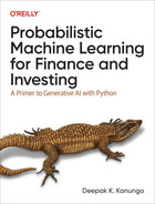
Let’s go back to the linear ensemble in the previous chapter and analyze the simulated 20,000 posterior predictive samples that our ensemble has generated using our model assumptions and the observed data. It is important to note that the posterior predictive distribution generates a range of possible future outcomes, each of which could have been generated by any combination of parameter values of our ensemble that is consistent with its model assumptions and the data used to train and test it.
While we can easily calculate descriptive statistics of the posterior predictive samples as we do later, we cannot directly associate any sample outcome with specific values of the model parameters. Of course, we can always infer the credible interval of each parameter that might have generated the samples from its marginal posterior distribution, as we did in the previous chapter. Let’s use the following Python code to summarize the predicted excess returns of a hypothetical position in Apple stock:
# Flatten posterior predictive xdarray into one numpy array of# 20,000 simulated samples.simulated_data=target_predicted.flatten()# Create a pandas dataframe to analyze the simulated data.generated_data=pd.DataFrame(simulated_data,columns=["Values"])# Print the summary statistics.(generated_data.describe().round(2))# Plot the predicted samples of Apple's excess returns generated by# tested linear ensemble.plt.hist(simulated_data,bins='auto',density=True)plt.title("Apple's excess returns predicted by linear ensemble")plt.ylabel('Probability density'),plt.xlabel('Simulated excess returns of Apple');
It is more important to note that this posterior predictive distribution of daily excess returns does not predict the specific timing or duration of those returns, only the distribution of possible returns in the future based on our ensemble’s model assumptions and data observed during the training and testing periods. Our ensemble average is the expected value of our hypothetical investment in Apple stock. Let’s see if it can help us decide whether to hold, increase, or decrease our position size.
A simple loss function, L(R, D″), is simply the market value of our position size multiplied by the daily excess returns of Apple for each simulated data point from the posterior predictive distribution of the ensemble:
-
L(R, D″) = R × D″
-
R is the market value of our investment in Apple stock.
-
D″ is a simulated daily excess return generated by our linear ensemble.
-
In the following Python code, we assume that our hypothetical investment in Apple stock is valued at $100,000 and compute the ensemble average of all simulated excess returns:
#Market value of position size in the portfolioposition_size=100000#The loss function is position size * excess returns of Apple#for each prediction.losses=simulated_data/100*position_size#Expected loss is probability weighted arithmetic mean of all the losses#and profitsexpected_loss=np.mean(losses)#Range of losses predicted by tested linear ensemble.("Expected loss on investment of $100,000 is ${:.0f}, with max possiblelossof${:.0f}andmaxpossibleprofitof${:.0f}".format(expected_loss,np.min(losses),np.max(losses)))Expectedlossoninvestmentof$100,000is$-237,withmaxpossiblelossof$-10253andmaxpossibleprofitof$8286
The expected value of –$237 is almost a rounding error based on an investment of $100,000. This suggests we can expect to experience little or no losses if we hold our position, assuming market conditions remain approximately the same as those encoded in our model and reflected in the observed data used to train and test it. Given the large range of possible daily losses and profits our position might incur over time, from –10.25% to +8.29%, isn’t the expected value of –0.24% misleading and risky? It seems that an ensemble average or expected value is a useless and dangerous statistic for risk management decisions. Let’s dig deeper into the statistical concept of expected value to understand why and how we can apply it appropriately.3
Recall that when we estimate the expected value of any variable, such as an investment, we compute a probability weighted average of all possible outcomes and their respective payoffs. We also assume that the outcomes are independent of one another and are identically distributed, i.e., they are drawn from the same stochastic process. In other words, the expected value of the investment is a probability-weighted arithmetic mean. What is noteworthy is that the expected value has no time dependency and is also referred to as the ensemble average of a stochastic process or system. If you have an ensemble of independent and identically distributed investments or trades you are going to make simultaneously, expected value is a useful tool for decision making. Or if you are running a casino business, you can calculate the expected value of your winnings across all gamblers at any given time.
However, as investors and traders, we only observe a specific path or trajectory that our investment takes over time. We measure the outcomes and payoffs of our investment sequentially as a time average over a finite period. In particular, we may only observe a subset of all the possible outcomes and their respective payoffs as they unfold over time. In the unlikely scenario that our investment’s trajectory realizes every possible predicted outcome and payoff over time, the time average of the trajectory will almost surely converge to the ensemble average. Such a stochastic process is called ergodic. We discussed this briefly in Chapter 6 in the Markov chain section.
What is special about an ergodic investment process is that the expected value of the investment summarizes the return observed by any investor holding that investment over a sufficiently long period of time. Of course, as was mentioned in Chapter 6, this assumes that there is no absorbing state in the Markov chain that truncates the investor’s wealth trajectory. As we will see in this section and the next, investment processes are non-ergodic, and relying on expected values for managing risks or returns can lead to large losses, if not financial ruin.
Even if a process is assumed to be ergodic, the time average of our investment does not take the actual ordering of the sequence of outcomes and payoffs into account. Why should it? After all, it’s just another arithmetic mean. What is noteworthy is that this, too, assumes that investors are passive, buy-and-hold investors. The specific sequence of returns that an investment follows in the market is crucial as it leads to different consequences and decisions for different types of investors. An example will help illustrate this point.
A stock trajectory that has a loss of –10.25% followed by a gain of +8.29% entails different decisions and consequences for an investor than a stock trajectory that has a gain of +8.29% followed by a loss of –10.25%. This is despite the fact that in both these two-step sequences the stock ends up down at –2.81% for a buy and hold investor. This up and down returns sequence is called volatility drag as it drags down the expected returns, an arithmetic mean, to the geometric mean, or compounded returns. If the volatility drag is constant, compounded returns = average return - 1/2 variance of returns. But the risks from the volatility drag for an investor could be very different depending on their investment strategy. Let’s see why.
Assume that for any stock position in their portfolio, an investor has a daily loss limit of –10% and a daily profit limit of +5%. The former stock sequence (–10.25%, +8.29%) will hit the investor’s stop-loss limit order at –10% and force them out of their position. To add insult to injury, the next day the stock comes roaring back +8.29%, while the investor is nursing a –10% realized loss on their investment. Now the investor would be down –7.19% compared to their peers who held onto their position or other investors who had a risk limit of –10.26% or lower. Talk about rubbing salt into our investor’s wounds! It would now be hard for the investor to decide to re-enter their position after such a bruising whiplash.
Let’s now consider what happens if the stock follows the latter sequence (+8.29%, –10.25%). The investor would take a profit of +5% when the stock shoots up +8.29%. They would feel some regret about not selling out of their position at the recent high price. But no one ever times the market perfectly or can do it consistently. However, the next day the investor would feel extremely smart and pleased with themselves when the stock falls –10.25%. They would be outperforming their peers by +7.81% and can gloat about it if they so choose. It would now be quite easy for the investor to re-enter their position in the stock since their break-even price would have been lowered by +5%.
This example demonstrates another reason why volatility, or standard deviation of returns, is a nonsensical measure of risk, as was discussed in Chapter 3. Volatility is just another ensemble average and is non-ergodic. In the first trajectory volatility hurts the investor’s returns, and in the second trajectory it helps them.
While the numbers are specific to our probabilistic ensemble, investment trajectories over any time period can be profoundly consequential to most active investors and traders in general. The specific ordering of return sequences impacts an investor’s decisions, experiences, and investment success. The concept of the “average investor” experiencing the expected value of returns on an investment is just another financial fairy tale.
Generative Value at Risk
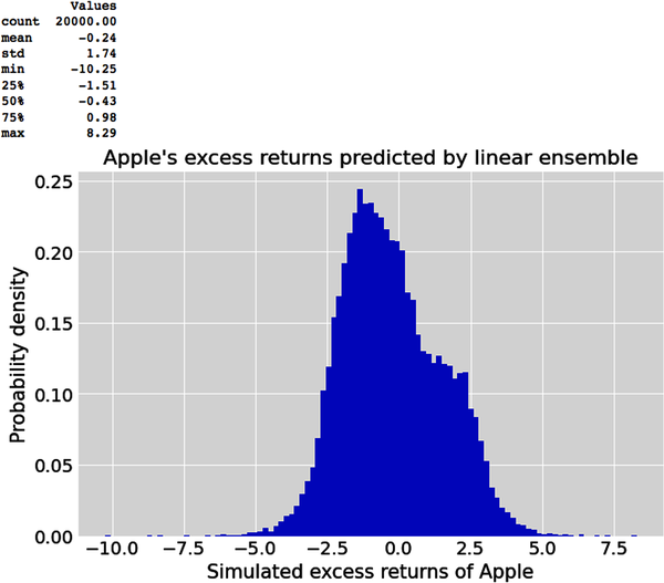
Rather than relying on the ensemble average, a popular loss function called value at risk (VaR) can help us make better risk management decisions for any time period. VaR is a percentile measure of a return distribution, representing the value below which a given percentage of the returns (or losses) fall. In other words, VaR is the maximum loss that is expected to be incurred over a specified period of time with a given probability. See Figure 8-1, which shows VaR and conditional VaR (CVaR), which is explained in the next subsection.
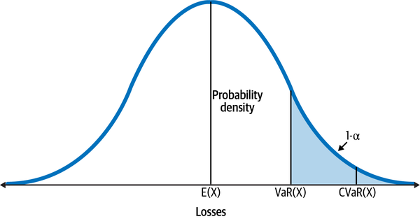
Figure 8-1. Value at risk (VaR) with alpha probability and conditional VaR (CVaR), also known as expected shortfall (ES), with 1-alpha probability shown for a distribution of returns of a hypothetical investment4
Unlike volatility, this measure is based on a commonsensical understanding of risk. As an example, say the daily VaR for a portfolio is $100,000, with 99% probability. This means that we estimate that there is a:
-
99% probability that the daily loss of the portfolio will not exceed $100,000
-
1% probability that the daily loss will exceed $100,000
Generally speaking, the time horizon of VaR is often related to how long a decision maker thinks might be necessary to take an action, such as to liquidate a stock position. Longer time horizons generally produce larger VaR values because there is more uncertainty involved the further out you go into the future.
In Chapter 3, we used Monte Carlo simulation to expose the deep flaws of using volatility as a measure of risk. It is common in the industry to use Monte Carlo simulations to estimate VaR for complex investments or portfolios using theoretical or empirical models. The risk estimate is called Monte Carlo VaR. In probabilistic machine learning, this simulation is done seamlessly and epistemologically consistently using the posterior predictive distribution. I use posterior predictive samples to estimate VaR, which I call Generative VaR or GVaR, as follows:
-
Sort N simulated excess returns in descending order of losses.
-
Take the first M of those losses such that 1 − M/N is the required probability threshold.
-
The smallest loss in the subset of M losses is your GVaR.
Now let’s use Python to compute the GVaR of our linear ensemble from the losses in the tail of its posterior predictive distribution:
#Generate a list the 20 worst daily losses predicted# by tested linear ensemble.sorted_returns=generated['Values'].sort_values()sorted_returns.head(20).round(2)
# Compute the first percentile of returns.probability=0.99gvar=sorted_returns.quantile(1-probability)(f"The daily Generative VaR at{probability}% probability is{gvar/100:.2%}implyingadollarlossof${gvar/100*position_size:.0f}")ThedailyGenerativeVaRat0.99%probabilityis-3.79%implyingadollarlossof$-3789
Generative Expected Shortfall
After the Great Financial Crisis, it became common knowledge that there is a deep flaw in the VaR measure that was used by financial institutions. It doesn’t estimate the heavy losses that can occur in the tail of the distribution beyond VaR’s cutoff point. Expected shortfall (ES), also known as conditional VaR, is a loss function that is commonly used to estimate the rare but extreme losses that might occur in the tail of the return distribution. Refer back to Figure 8-1 to see the relationship between VaR and ES. As the name implies, ES is an expected value and is estimated as a weighted average of all the losses after the VaR’s cutoff point. Let’s compute the generative ES of our linear ensemble and compare it to all the worst returns in the tail of the posterior predictive distribution:
# Filter the returns that fall below the first percentilegenerated_tail=sorted_returns[sorted_returns<=gvar]# Expected shortfall is the mean of the tail returns.ges=generated_tail.mean()# Generated tail risk is the worst possible loss predicted# by the linear ensemblegtr=generated_tail.min()# Plot a histogram of the worst returns or generated tail risk (GTR)plt.hist(generated_tail,bins=50)plt.axvline(x=gvar,color='green',linestyle='solid',label='Generative Value at Risk')plt.axvline(x=ges,color='black',linestyle='dashed',label='Generative expected shortfall')plt.axvline(x=gtr,color='red',linestyle='dotted',label='Generative tail risk')plt.xlabel('Simulated excess returns of Apple')plt.ylabel('Frequency of excess returns')plt.title('Simulation of the bottom 1% excess returns of Apple')plt.legend(loc=0)plt.show()(f"The daily Generative VaR at{probability}% probability is{gvar/100:.2%}implyingadollarlossof${gvar/100*position_size:.0f}")(f"The daily Generative expected shortfall at{1-probability:.2}%probabilityis{ges/100:.2%}implyingadollarlossof${ges/100*position_size:.0f}")(f"The daily Generative tail risk is{gtr/100:.2%}implyingadollarlossof${gtr/100*position_size:.0f}")

From the loss functions of VaR and ES, we can see that there is a 99% probability that the daily losses on our hypothetical investment in Apple stock is not expected to be lower than –3.79%. Should the loss exceed that GVaR threshold, the GES or daily loss in 1% of the scenarios is not expected to be lower than –4.50%.
Generative Tail Risk
The major flaw of ES is that it is yet another expected value or ensemble average that understates the risks due to extreme events. It’s an even more dangerous statistic as it is averaging over a subset of the worst losses of the returns of our regression ensemble in a region of the distribution that is even more non-ergodic and fat-tailed as shown in the previous graph of the simulated losses in the tail of the posterior predictive distribution. For our specific ensemble, the worst loss is over twice the GES. If an extreme loss impairs your capital base, you will not be around to observe the expected shortfall. As a volatility trader who is short volatility quite often, I use the worst loss generated by the posterior predictive distribution— –10.25% for our ensemble—as my shortfall and hedge my trades accordingly. I refer to it as the Generative tail risk (GTR) of the ensemble.
If you own a stock, as most people do, you are in essence short volatility and are making a high-probability bet that the stock is not going to make unexpected moves in the future. Based on your risk preferences, position size, and confidence in your regression ensemble, you might choose a different percentile in the tail of the return distribution as a reference point to manage your tail risk. Consequently, you may decide to hold your stock position, reduce it, or hedge it with options or futures or both. Regardless, you should continue to monitor your investment and the overall market by continually updating your regression ensemble with more recent data as it becomes available. As we have discussed in the latter half of this book, continual probabilistic machine learning is the hallmark of generative ensembles.
Capital Allocation
Capital preservation, or return of our capital, is our primary objective. In the previous section, we explored the tools we can use to manage our risky investments to achieve that objective. Now let’s focus our attention on the second objective: the return on our capital, or capital appreciation. As investors and traders, we have two related, fundamental decisions to make when faced with investing in risky assets in an environment of three-dimensional uncertainty and incomplete information:
-
Evaluate and decide if the investment will appreciate in value over a reasonable time period.
-
Decide what fraction of our hard-earned capital to allocate to that opportunity.
Expected value is used extensively for evaluating the attractiveness of investment opportunities. It is applied in almost every situation in finance and investing, from estimating the free cash flows of a company’s capital project to valuing its debt and its outstanding equity. However, like all concepts and tools, expected value has its strengths, weaknesses, and limitations. As we have already discussed in the previous section, expected value as an ensemble average is a complex idea. In this section we continue to deepen our understanding of ensemble averages to see if and where they can be applied appropriately by an investor looking to allocate their capital to increase their wealth without risking financial ruin at any time.
Gambler’s Ruin
It was not until the 17th century that Blaise Pascal, an eminent mathematician and physicist, working with a French aristocrat to improve his gambling skills, proved mathematically what was known to be true for a few millennia: eventually all gamblers go broke. Gambles are useful probabilistic models and have played a pivotal role in the development of probability and decision theories.6 The classic problem of gambler’s ruin is instructive for investors as it emphasizes that a positive expected value is a necessary condition for making investments.
Suppose you decide to play the following coin-tossing game. You start with $M, and your opponent starts with $N. Each of you bets $1 on the toss of a coin, which turns up heads with probability p and tails with probability q = (1 – p). If it’s heads, you win $1 from your opponent; if it’s tails, you lose $1 to your opponent. The game ends when either player goes broke (i.e., ruined). This is no silly game. It’s a stochastic process called an arithmetic random walk and can be used to model stock prices and collisions of dust particles. It is also a Markov chain, since its future state only depends on its current state and not the path it took to get there.
The gambler’s ruin is a two-part problem in which a gambler makes a series of bets with negative or zero expected value. Using the arithmetic random walk model, it can be shown mathematically that any gambler will almost surely go broke in both of the following scenarios:
-
A gambler makes a series of bets, where the probability of success for each bet is less than 50% and payoff equals the amount staked. In such games the gambler will eventually go broke regardless of their betting strategy since their wager always has negative expectation. It doesn’t even matter how big the gambler’s bankroll is compared to their opponents. The gambler’s probability of ruin P(ruin) is:
-
A gambler is given a series of bets where the probability of success of each bet is 50% and the payoff equals the amount staked. These are fair odds, but the gambler’s opponent has a bigger bankroll. Surprisingly, the gambler will eventually go broke even in this scenario, if their opponent has a marginally bigger bankroll. If their opponent has a much larger bankroll, such as a casino dealer, the bumpy road to ruin transforms into a highway with no speed limit. The probability of ruin P(ruin) is:
-
Note that in the first scenario, we are assuming that the gambler is not able or allowed to count cards or use the physics of the gambling machine, such as a roulette wheel, as the great Ed Thorp did to beat the dealers in Vegas in the 1960s.7
The math is brutally clear. No matter how hard you try or what betting system you invent, because of negative expectations of the bets, gambling is a fool’s errand for the ages. Gamblers will take all kinds of random walks that will zig and zag between gains and losses, but all roads will eventually lead to ruin. Games involving equal odds with equal bankrolls are implausible situations for almost all gamblers. So to avoid going broke, a gambler needs to make bets with positive expected values.
But a gamble with positive expectation is commonly known as an investment. In mathematical models, the sign of the expected value of each bet is the main difference between a gamble and an investment, according to John Kelly, the inventor of the optimal capital growth algorithm.8 By engaging in positive expectation bets, a degenerate gambler morphs into a respectable investor who can now pursue a statistically feasible path of increasing their wealth while avoiding financial ruin. But what fraction of our capital do we allocate to investments with positive expectations? Does it make sense to go all in when we are offered really favorable odds?
Expected Valuer’s Ruin
Say you are confronted by a wealthy and powerful adversary who owns a biased coin that has a 76% probability of showing heads. Assume that the probability of this biased coin is known precisely to all, but the physics of any coin toss is always unknown. Your adversary makes you a legally binding offer—an offer you can refuse.
If you stake your entire net worth on a single toss of his coin and it shows heads, he will pay you three times the value of your net worth. But if the coin shows tails, you lose your entire net worth except the clothes you are wearing—it’s not personal, it’s just business. This seems like the wager of a lifetime because it gives you the opportunity to increase your net worth twofold in a blink of an eye:
-
Expected value of wager = (3 × net worth × 0.76) – (net worth × 0.24) = 2.04 × net worth.
-
Payoffs are in multiples of your net worth, which will get estimated in legal proceedings (or not), so bluffing your net worth won’t help.
Do you accept this offer, which clearly has a high expected value, with a 76% probability of success but with a nontrivial 24% probability of financial ruin? Tossing a coin once doesn’t really involve time, so can expected value as an ensemble average work here to help us evaluate this opportunity?
Our common sense instinctively raises red flags about relying on any financial rule of maximizing expected value for such high-stakes decision making. It’s as if we were the ones staring down the barrel of Detective “Dirty” Harry’s famous .44 magnum handgun, wondering whether there is a bullet left, and him warning us: “You’ve gotta ask yourself one question: ‘Do I feel lucky?’ Well, do ya, punk?”
Any responsible person, experienced investor, trader, or corporate executive (all of whom, generally speaking, are not punks) would refuse this offer because any investment opportunity that even hints at the possibility of financial ruin is a deal-breaker. This is expressed succinctly in a market maxim that says, “There are old traders, there are bold traders, but there are no old, bold traders.” Or another one that says, “Bulls make money, bears make money, but pigs get slaughtered.” One essential statistical insight of these two aphorisms, built over centuries of collective observations and life experiences, is that maximizing the expected value of investments almost surely leads to heavy losses, if not financial ruin, even if the odds are in your favor.
What about a series of favorable bets where you maximize the expected value of each bet by going all in? Even if your same adversary were to give you a series of independent and identically distributed (i.i.d.) positive expectation bets, it would be ruinous for you to bet everything you have on each successive bet. You don’t need mathematical proof to figure out that it only takes one losing bet to wipe out all the accumulated profits and the initial bankroll of any investor who is an expected value maximizer.
So how should you make your decision in one-off binary opportunities with positive expectations that don’t involve betting your entire net worth? Let’s return to the situation we described in Chapter 6 regarding ZYX technology company and its earnings expectations. Recall that after observing ZYX successfully beat its earnings expectations in the last three quarters, your model’s prediction was that there was a 76% probability that it would beat its earnings expectations in the next quarter. Assume that you continue to find the probabilistic model useful, and ZYX is going to announce its earnings after the close of trading today.
Based on prices of options traded on ZYX stock, it seems that the market is pricing a 5% move up in the stock price if ZYX beats its earnings expectations. However, the market is also pricing a 15% move down in ZYX stock price if it does not. For the sake of this discussion, assume that these are accurate forecasts of the move in the stock prices after the earnings event. How can you use this market information and your model’s prediction to allocate capital to ZYX stock before the earnings announcement today?
Let’s create an objective function V(F, Y″) where F is the fraction of your total capital you want to invest in ZYX and Y″ is the predicted outcome of an earnings beat. Given your objectives of avoiding any possibility of penury, F must be in the interval [0, 1):
-
Since F cannot equal 1 for any investment, we avoid the expected value maximizing strategy and the gambler’s ruin, as previously discussed.
-
Furthermore, leveraging your position is not allowed as F < 1. This means you cannot borrow cash from your broker to invest more capital than the cash in your account. When you borrow money from your broker to invest in stocks, you can end up owing more than your initial capital outlay, which is worse than blowing up your account.
-
Since F cannot be negative, you cannot short stocks. Shorting a stock is an advanced trading technique in which you borrow the shares from your broker to sell the stock with the expectation of buying it at a lower price. It’s buying low and selling high but in reverse order. Note that stock prices have a floor at $0 because of the limited liability of corporate ownership. However, stocks do not have a theoretical upper limit, which many unfortunate investors have realized in bubbles and manias. This is why shorting stocks can be risky and requires expertise and disciplined risk management. Stocks can burst into powerful rallies, called short covering rallies, for the flimsiest of reasons. These rallies can be twice as powerful, since there are buy orders from buyers and buy orders from short sellers, who are rushing to cover their short positions by buying back the stocks they had previously sold short. I have been on the wrong side of such short covering rallies several times, and the phrase “face-ripping rallies” is a fitting description of these experiences.
Recall that Y″ is our probabilistic model’s out-of-sample predictions of ZYX’s earnings announcements based on observed in-sample data D, with P(Y1″ = 1 | D) = 76% when ZYX beats earnings expectations and P(Y0″ = 0 | D) = 24% when it doesn’t. Therefore, the expected value of our objective function, E[V(F)], is the probability weighted average over a profit (W) outcome of 5% and a loss outcome (L) of –15%:
-
E[V(F)] = W × F × P(Y1″ = 1 | D) + L × F × P(Y0″ = 0 | D)
-
E[V(F)] = 0.05 × F × 0.76 – 0.15 × F × 0.24 = 0.002 × F
-
The trade has an edge or positive expectation of about 0.2%.
It only takes common sense to see that no single investor will observe an increase of 0.2% in the stock value of ZYX, or any other expected value they might have estimated, after the earnings event. Depending on the actual earnings results of ZYX, each investor who is long on the stock will either incur a 5% gain or –15% loss, or vice versa if they are short on the stock. The expected value we have computed is an ensemble average of all the profits and losses of all ZYX stockholders. It is hard to estimate, and it may or may not be within a reasonable range of your estimate.
But why should we care about the ensemble average anyway in this situation? As you can see, it is a completely useless tool for decision making in such one-off binary events for a single investor. A positive expected value of ZYX’s earnings event sounds great until you get hit with a –15% loss in a high-frequency microsecond, much faster than your eye can even blink. Mike Tyson, a former heavyweight boxing champion, summarized such hopeful positive expectations eloquently when he said, “Everyone has a plan until they get punched in the mouth.”
So what capital allocation algorithm can help you make decisions in one-off binary trades regardless of the amount of capital you are going to allocate to the bet? Unfortunately, there are none. Only your capacity to bear the worst known outcome of your decision, which is subjective by definition, can help you make such one-off binary decisions. We have already discussed how to integrate subjectivity into probabilistic decision making. Say you have a daily loss limit of –10% and daily profit limit of +5% for any position in your portfolio. This makes the decision systematic and much easier to make, especially for automated systems:
-
Don’t invest in ZYX before the earnings announcement, since the non-trivial probability of losing –10% in one day conflicts with the risk limits of your objective function.
-
Don’t short ZYX stock since that conflicts with your objective function.
-
If you already have an investment in ZYX stock, you need to recalibrate your position size and hedge it with options or futures such that the daily loss doesn’t exceed –10%. Of course, hedging costs will lower the 5% expected gain, so you will have to recalculate the expected value to make sure it is still positive.
Searching for investment opportunities that have positive expected values over a reasonable time horizon is generally the difficult part of any investment strategy. But in this section, we have learned that making investments with positive expectation is a necessary but not a sufficient condition. Therefore, investors are faced with a dilemma:
-
If they allocate too much capital to such a favorable opportunity, they risk bankruptcy or making devastating losses.
-
If they allocate too little capital, they risk wasting a favorable opportunity.
This implies that investors need a capital allocation algorithm that computes a percentage of their total capital to a series of investment opportunities with positive expectation such that it balances two fundamental objectives:
-
Avoids financial ruin at all times
-
Increases their wealth in a finite time period
Some investors have additional objectives that are to be achieved on the capital they manage over a specific time period, generally one year:
-
Percentage profits to exceed a defined threshold
-
Percentage losses not to exceed a defined threshold
These objectives can be encoded in an investor’s objective function that will condition and constrain their capital allocation algorithm. As we have already learned in this chapter so far, applying expected value in investing and finance is neither intuitive nor straightforward, as investment processes are non-ergodic. Let’s explore a capital allocation algorithm that is widely used in academia and in the industry.
Modern Portfolio Theory
Modern portfolio theory (MPT), developed by Harry Markovitz in 1952, focuses on quantifying the benefits of diversification using correlations of returns of different assets in a portfolio. It maximizes the expected value of the returns of a portfolio of assets for a given level of variance over a single time period, so volatility (the square root of variance) is used as a constraint on the expected value optimization algorithm. MPT assumes that asset price returns are stationary ergodic and normally distributed.
As we have learned already, these are unrealistic and dangerous assumptions, due to the following factors:
-
They ignore skewness and kurtosis of asset price returns, which are known to be asymmetric and fat-tailed even by academics.
-
Portfolio diversification is reduced or eliminated in periods of extreme market stress, as we saw recently in 2020 and previously in 2008.
-
In normal periods, fat-tailed distributions can introduce large errors in correlations among securities in the portfolio.
-
Portfolio weights can be extremely sensitive to estimates of returns, variances, and covariances. Small changes in return estimates can completely change the composition of the optimal portfolio.
MPT portfolios are much riskier than advertised and provide suboptimal returns—diversification leads to “diworsification.” Buffet has called MPT “a whole lot of nonsense” and has been laughing all the way to his mega bank ever since.
In an interview, Markowitz admitted to not using his “Nobel prize–winning” mean-variance algorithm for his own retirement funds! If that is not an indictment of the mean-variance algorithm, I don’t know what else is.9 Instead Markowitz used 1/N heuristic or the naive diversification strategy. This is an investment strategy in which you allocate equal amounts of your capital to each of N investments. This naive diversification portfolio strategy has been shown to outperform mean variance and other complex portfolio strategies.10
We focus our attention on another simpler but equally useless model of MPT to highlight the conceptual blunder of using volatility as a measure of total risk. The capital asset pricing model (CAPM) discussed in Chapter 4 was derived from Markovitz’s portfolio theory by his student William Sharpe. It simplifies MPT in terms of thinking about expected return for any risky investment. According to the CAPM, an asset has two types of risks: unsystematic and systematic. Unsystematic risk is idiosyncratic to the asset concerned and is diversifiable. Systematic risk is market risk that affects all assets and is not diversifiable.
The CAPM builds on the heroic assumptions of MPT that all investors are rational and risk-averse and have the same expectations at the same time given the same information, such that markets are always in equilibrium. Such financial fairy tales rival any you might see in Disney’s Magic Kingdom. At any rate, these Markovitz investors are supposed to create strongly efficient markets and only hold diversified portfolios that will reduce the correlation among assets and eliminate the idiosyncratic risk of any particular asset. Statistically, this implies that in a well-diversified portfolio, the idiosyncratic risk of any particular asset will be zero, as will the expected value of any error term in the regression line. Therefore, Markovitz investors will only pay a premium for systematic risk of an asset, as it cannot be diversified away.
In such strongly efficient markets, all fairly priced investments will plot on a regression line called the security market line with the intercept equal to the risk-free rate and the slope equal to beta, or systematic risk. An asset’s beta gives the magnitude and direction of the movement of the asset with respect to the market. See Figure 8-2 (M is the market portfolio with beta = 1).
The systematic risk term, beta, of the asset’s MM is the same as the one calculated using its CAPM. However, note that an asset’s market model (MM) is different from its CAPM in three important respects:
-
The CAPM formulates expected returns of an asset, while its MM formulates realized returns.
-
The MM has both an idiosyncratic risk term (alpha) and an error term in its formulation.
-
Based on MPT, the expected value of alpha is zero since it has been diversified away by rational investors. That is the reason it does not appear in the CAPM.
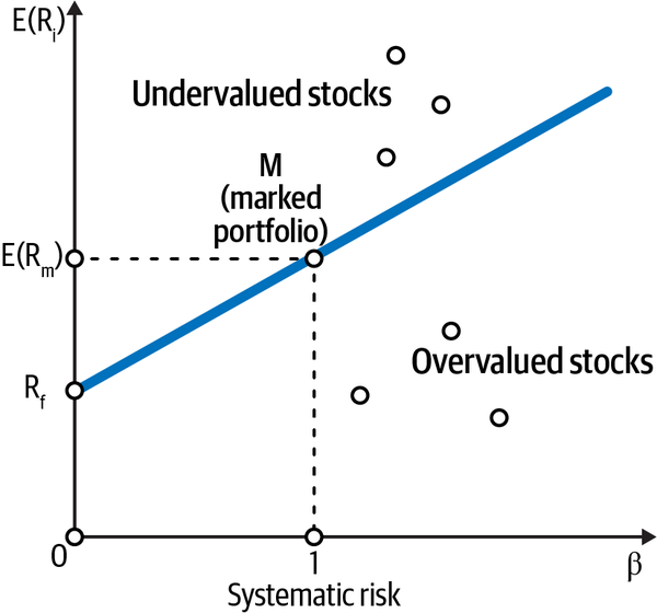
Figure 8-2. The CAPM claims that as you increase the systematic risk of your investment, or beta, its expected return increases linearly. Beta is directly proportional to the volatility of returns of the investment11
In simple linear regression, beta quantifies the average change in the target for a unit change in the associated feature. Based on the assumptions of simple linear regression, especially the one about constant variance of the residuals, beta has an analytical formula that is equal to:
-
Beta = Rxy × Sy / Sx where:
-
Sy = standard deviation of the target or investment
-
Sx = standard deviation of the feature or market portfolio
-
Rxy = coefficient of correlation between the feature and the target
-
Beta can also be interpreted as the parameter that correlates the volatility of the risky investment with the volatility of the market.
Markowitz Investor’s Ruin
As you can see from Figure 8-2, the CAPM claims that you can increase the expected value of returns as much as you want, by selecting risky investments or using leverage or both, as long as you are willing to accept the attendant volatility of the asset’s price returns.
Let’s test these assumptions about the expected value of returns by generating a very large sample of hypothetical trades with the same probabilities, outcomes, and payoffs as ZYX’s earnings event. In the following Python code, we generate 20,000 samples from our posterior predictive distribution. That should be sufficiently large for the law of large numbers (LLN) to kick in and enable the convergence of any asymptotic property of stochastic processes.
In particular, we will calculate our ensemble average by computing the posterior predictive mean across the 20,000 simulated samples. These samples simulate the two outcomes of ZYX’s earnings event. We then provide the same 20,000 outcomes sequentially as a time series to 100 simulated investors. Each simulated investor applies MPT/CAPM theory to their investing process. They allocate anywhere from 1% to 100% of their initial capital of $100,000 to ZYX stock. The profit or loss resulting from each of the simulated outcomes for a specific investor/fraction of the total capital is computed. Our code keeps track of the terminal wealth for each specific fraction/investor iteratively. Finally, we plot the terminal wealth for each fraction/investor and check if the time average of the typical investor equals the ensemble average computed earlier:
#Fix the random seed so numbers can be reproducednp.random.seed(114)#Number of posterior predictive samples to simulateN=20000#Draw 100,000 samples from the model's posterior distribution#of parameter p#Random.choice() selects 100,000 values of p from the#earnings_beat['parameter'] column using the probabilities in the#earnings_beat['posterior'] column.posterior_samples=np.random.choice(earnings_beat['parameter'],size=100000,p=earnings_beat['posterior'])#Draw a smaller subset of N random samples from the#posterior samples of parameter pposterior_samples_n=np.random.choice(posterior_samples,size=N)#Generate N random simulated outcomes by using the model's likelihood#function and posterior samples of the parameter p#Likelihood function is the Bernoulli distribution, a special case#of the binomial distribution where number of trials n=1#Simulated data are the data generated from the posterior#predictive distribution of the modelsimulated_data=np.random.binomial(n=1,p=posterior_samples_n)#Plot the simulated data of earnings outcomes y=0 and y=1plt.figure(figsize=(8,6))plt.hist(simulated_data)plt.xticks([0,1])plt.xlabel('Predicted outcomes')plt.ylabel('Count')plt.title('Simulated outcomes of ZYX beating earnings expectations')plt.show()#Count the number of data points for each outcomey_0=np.sum(simulated_data==0)y_1=np.sum(simulated_data==1)#Compute the posterior predictive distribution(f"Probability that ZYX will not beat earnings expectations (y=0) is:{y_0/(y_0+y_1):.3f}")(f"Probability that ZYX will beat earnings expectations (y=1) is:{y_1/(y_0+y_1):.3f}")
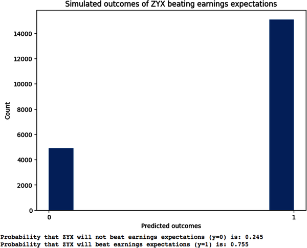
Notice that the probabilities of the outcome variables based on our posterior predictive distribution are almost equal to the theoretical probabilities for y = 0 and y = 1. This validates our claim that the sample size is large enough for asymptotic convergence and the LLN is working as expected. Now we continue to calculate our profits and losses based on a sequence of 20,000 possible outcomes generated by our model to compute the terminal wealth of all investors:
#Percentage losses when y=0 and earnings don't beat expectationsloss=-0.15#Percentage profits when y=1 and earnings beat expectationsprofit=0.05#Set the starting capitalstart_capital=100000#Create a list of values for position_size or percentage of total capital#invested in ZYX by an investorposition_size=np.arange(0.00,1.00,0.01)#Create an empty list to store the final capital values for#each position_size of an investorfinal_capital_values=[]#Loop over each value of position_size f to calculate#terminal wealth for each investorforfinposition_size:#Set the initial capital for this simulationcapital=start_capital#Loop over each simulated data point and calculate the P&L based on y=0 or y=1foryinsimulated_data:ify==0:capital+=capital*loss*felse:capital+=capital*profit*f# Append the final capital value to the listfinal_capital_values.append(capital)#Find the value of f that maximizes the final capital of each investoroptimal_index=np.argmax(final_capital_values)optimal_f=f_values[optimal_index]max_capital=final_capital_values[optimal_index]#Plot the final capital values as a function of position size, fplt.figure(figsize=(8,6))plt.plot(position_size,final_capital_values)plt.xlabel('Position size as a fraction of total capital')plt.ylabel('Final capital values')plt.title('Growth of total capital as a function of position size in ZYX')# Plot a vertical line at the optimal value of fplt.axvline(x=optimal_f,color='red',linestyle='--')plt.show()#Print the optimal value of f and the corresponding final capital(f"The optimal fraction of total capital is{optimal_f:.2f}")(f"Initial capital of ${start_capital:.0f}grows to afinalcapitalof${max_capital:.0f}")
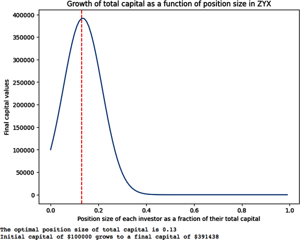
We can make a few obvious observations based on our simulation:
-
Investors experience different wealth trajectories based on the fraction of the initial capital they invested in this series of hypothetical positive expectation bets (total of 20,000 i.i.d. bets).
-
Investors start losing money if they invested more than 26% of their capital.
-
All investors who invested more than 40% of their capital are broke.
-
All investors who invested between 1% to 26% of their capital increased their wealth.
-
The investor who invested only 13% of their capital had the greatest amount of terminal wealth. In this investment scenario, 13% of total capital is the Kelly optimal position size for growing one’s wealth.
-
It is important to note that an investor’s risk of ruin is closely related to the position size of their initial capital and not to the volatility of returns of the stochastic process, which is the same for every investor.
-
Most importantly, even if you are willing to accept the related volatility of your investment, there is a limit to how much capital you should allocate to an investment. This is the fatal flaw of MPT/CAPM and reveals the foolishness of using volatility as a measure of risk.
As shown in our simulation, assuming that investing is an ergodic process and optimizing expected value leads to financial ruin for the majority of the investors applying MPT/CAPM principles of using volatility as a proxy for risk and disregarding position size. This is how LTCM justified leveraging its positions arbitrarily highly and disregarding the possibility of financial ruin.
Kelly Criterion
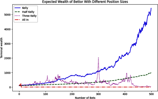
In 1956, John Kelly, a physicist working at Bell Labs, came up with the groundbreaking solution to the vexing problem of how much is optimal to invest in positive expectation opportunities following a non-ergodic stochastic process. His solution, commonly referred to as the Kelly criterion, is to maximize the expected compound growth rate of capital, or the expected logarithm of wealth.12 The Kelly position size is the optimal amount of capital allocated to a sequence of positive expectation bets or investments that results in the maximum terminal wealth in the shortest amount of time without risking financial ruin.
Say your wealthy adversary gives you another weighted coin that has a 55% probability of turning up heads. He offers you an infinite series of trades with even odds:
-
On heads, you get two times your stake. On tails, you lose your entire stake.
-
How much capital do you allocate to maximize your capital in the long term?
Let’s run a simulation in Python of a simple series of binary bets with fixed odds to illustrate the power of the Kelly criterion for maximizing your wealth:
importnumpyasnpimportmatplotlib.pyplotaspltnp.random.seed(101)# Weighted coin in your favorp=0.55# The Kelly position size (edge/odds) for odds 1:1f_star=p-(1-p)# Number of series in Monte Carlo simulationn_series=50# Number of trials per seriesn_trials=500defrun_simulation(f):#Runs a Monte Carlo simulation of a betting strategy with#the given Kelly fraction.#Takes f, The Kelly fraction, as the argument and returns a NumPy array#of the terminal wealths of the simulation.# Array for storing resultsc=np.zeros((n_trials,n_series))# Initial capital of $100c[0]=100foriinrange(n_series):fortinrange(1,n_trials):# Use binomial random variable because we are tossing# a weighted coinoutcome=np.random.binomial(1,p)# If we win, we add the Kelly fraction to our accumulated capitalifoutcome>0:c[t,i]=(1+f)*c[t-1,i]# If we lose, we subtract the Kelly fraction from# our accumulated capitalelse:c[t,i]=(1-f)*c[t-1,i]returnc# Run simulations for different position sizes# The Kelly position size is our optimal betting sizec_kelly=run_simulation(f_star)# Half Kelly size reduces the volatility while keeping the gainsc_half_kelly=run_simulation(f_star/2)# Anything more than twice Kelly leads to ruin in the long runc_3_kelly=run_simulation(f_star*3)# Betting all your capital leads to ruin very quicklyc_all_in=run_simulation(1)# Plot the expected value/arithmetic mean of terminal wealth# over all the iterations of 500 trials eachfig,ax=plt.subplots(figsize=(10,6))# Overlay multiple plots with different line styles and markersax.plot(c_kelly.mean(axis=1),'b-',lw=2,label='Kelly')ax.plot(c_half_kelly.mean(axis=1),'g--',lw=2,label='Half Kelly')ax.plot(c_3_kelly.mean(axis=1),'m:',lw=2,label='Three Kelly')ax.plot(c_all_in.mean(axis=1),'r-.',lw=2,label='All In')ax.legend(loc=0)ax.set_title('Expected Wealth of Bettor With Different Position Sizes')ax.set_ylabel('Terminal wealth')ax.set_xlabel('Number of Bets')plt.show()
For binary outcomes, an investor can compute the percentage of capital, F, to be allocated to an opportunity with positive expectation in the real world of non-ergodic investing processes. However, the popular literature on the Kelly criterion doesn’t provide the general Kelly position sizing formula that you can apply to investments or bets in which you lose a percentage of your stake and not your entire stake. The optimal fraction, F′, is:
-
F′ = (W × p – L × q) / (W × L) where
-
p is the probability of gain and q = 1 – p is the probability of loss.
-
W is percentage gain and L is the percentage loss.
-
-
Note when L = 1, you lose your entire stake and you get the popular formula:
-
F′ = (W × p – q) / W, or as it is popularly known, edge over odds.
-
This formula is used in sports betting, where you can lose your entire stake.
-
It is important to note that the Kelly formula relates the ensemble average to the time average of a single trajectory. The expected value, or edge, of the investment is in its numerator. But the denominator modifies the position size implied by the ensemble average by including the multiplicative losses and profits that will be incurred sequentially in the time average. This is the volatility drag we discussed in the ergodicity subsection earlier.
The Kelly formula solves the gambler’s ruin problem for multiplicative dynamics quite elegantly. Recall that the gambler’s ruin problem involves a series of additive bets. In contrast, the Kelly criterion is used for a series of multiplicative bets. When the expected value or edge of an opportunity is zero, the Kelly formula gives it a zero position size. Furthermore, when the expectation is negative, the position size is also negative. This implies you should take the other side of the bet. In gambling, this would mean betting against gamblers and with the casino dealer. In markets, it means betting that markets will fall and taking a short position in an investment.
The Kelly criterion has many desirable properties for investing in positive expectation investment opportunities:13
-
It is mathematically indisputable that the Kelly position maximizes the terminal wealth in the shortest amount of time without the risk of going broke.
-
It generates exponential growth since profits are reinvested.
-
It involves a multiperiod, myopic trading strategy where you can focus on the present opportunities without a need for a long-term plan.
-
-
It has risk management built into the formula:
-
Kelly position size is a fraction of your capital.
-
Position size becomes smaller as losses accumulate.
-
The Kelly criterion expressed mathematically that evaluating expected values of investment opportunities is necessary but not sufficient. Sizing our investment position to account for the non-ergodic process of investing is of paramount importance and the sufficient condition we need. Unfortunately, capital allocation in financial markets is not that simple, and applying the Kelly criterion is challenging because markets are not stationary.
Kelly Investor’s Ruin
As we have mentioned in Chapter 1, financial markets are not only non-ergodic, but they are also nonstationary. The underlying data-generating stochastic processes vary over time. This makes estimating the continually changing statistical properties of these processes hazardous, especially when the underlying structure of the market changes abruptly.
Note that the posterior predictive distribution of the outcome variable Y″, the event that ZYX will beat earnings expectations, has a probability distribution due to the uncertainty of its parameter and data sampling. The 76% probability is just the mean value of its posterior predictive distribution. The expected value of our objective function turns negative if our estimate is less than 75%. There is not much margin for error here, and that should raise red flags. Based on the analytical formula and theoretical probability of an earnings beat of 75%, the Kelly position size should be zero. However, we have overshot the Kelly position, and our capital growth is suboptimal but positive for this simulation. It is quite possible that for another simulation with more samples, the position size changes and the current position size of 13% would lead to ruin.
The Kelly position sizing formula is very sensitive to estimates of both the expected value (the “edge”) and the probabilities of gains and losses (the “odds”). The cardinal sin in applying the Kelly formula is to overbet or to have a position size larger than the Kelly size. As an investor’s position size goes past the Kelly optimum, the growth rate of their wealth decreases and inexorably moves them toward financial ruin.14
Practitioners of the Kelly criterion use a fraction of the Kelly optimal size, such as half Kelly, to avoid overbetting, as it hedges against:
-
Overestimating one’s edge
-
Misestimating event odds
-
Changing edge and odds
Fractional Kelly allocation strategies also reduce the volatility of returns that can accompany full Kelly position sizes. The full application of the Kelly criterion to a portfolio of investments involves nonlinear programming and is beyond the scope of this primer.15
Summary
Complex decision making in the real world is an art and a science. Our probabilistic decision framework gives us the perspective and the tools to integrate our prior knowledge and subjective reasons with the objectivity of observed data and the unrelenting rigors of probability calculus. It enables us to make the best decisions that optimize our objectives in the face of uncertainty and incomplete information. To make such systematic decisions that we can entrust to machines, we need to specify an objective function and evaluate the function based on all possible outcomes generated from the posterior predictive distribution of our generative ensembles.
Expected value, also known as an ensemble average, needs to be applied with great caution because finance and investing processes are non-ergodic. Since each investor’s wealth trajectory is unique and different from the ensemble average computed across all possible trajectories of all market participants, their time average is not the same as the expected value of the ensemble. Also, different sequences of events lead to different decisions and outcomes even though the time average may be equivalent. In risk management, it is prudent to use value at risk instead of volatility, as VaR is estimated from the distribution of possible returns. Furthermore, it is better to use a tail-risk value instead of expected shortfall as that, too, is an ensemble average. My generative versions of these risk measures are produced seamlessly by probabilistic ensembles as I have demonstrated in this chapter.
The expected value of investments is a useful evaluation tool because it separates gambling from investing. However, while positive expectation is a necessary condition for investing, it is not a sufficient condition in a non-ergodic world. You need a capital allocation algorithm to appropriately size your investment so that you don’t go broke on any wealth trajectory your investment takes and you have a realistic chance of growing your wealth.
If you are looking to maximize the growth of your capital, you might want to consider the Kelly investment strategy, which outperforms any other capital allocation strategy, especially the suboptimal Markowitz’s mean-variance investment strategy. The Kelly criterion investment strategy has been used by the most successful investors of all time, including Warren Buffet, Ed Thorp, and James Simons. It is a travesty that the Kelly criterion is not taught in academia or professional programs. However, the Kelly formula is not a silver bullet and is hard to implement in a nonstationary world. That’s why most practitioners like me use fractional Kelly trading strategies to avoid overbetting and the risk of ruin.
Unfortunately, there are no easy formulas or algorithms for success in trading, investing, and finance that can be encoded in any AI system, because markets are not stationary ergodic. Symbolic AI and probabilistic machine learning systems require human common sense and expertise to separate correlation from causation to successfully navigate the aleatory, epistemic, and ontological uncertainties produced by creative, emotional, and free-willed market participants. Now that is a generative ensemble that can almost surely put the odds in your favor.
References
Bhide, A. V. “Compulsive Gambling in Ancient Indian Texts.” Indian Journal of Psychiatry 49, no. 4 (2007): 294–95.
Bower, Bruce “Simple Heresy: Rules of Thumb Challenge Complex Financial Analyses.” Science News 179, no. 12 (2011): 26–29.
DeMiguel, Victor, Lorenzo Garlappi, and Raman Uppal. “Optimal Versus Naïve Diversification: How Inefficient is the 1/N Portfolio Strategy?” Review of Financial Studies 22, no. 5 (2009): 1915–53.
Karasan, Abdullah. Machine Learning for Financial Risk Management with Python. O’Reilly Media, 2021.
Kelly Jr., J. L. “A New Interpretation of Information Rate.” The Bell System Technical Journal 35, no. 4 (1956): 917–26.
MacLean, L. C., E. O. Thorp, and W. T. Ziemba. “Long-Term Capital Growth: Good and Bad Properties of the Kelly Criterion.” Quantitative Finance 10, no. 7 (2010): 681–687.
MacLean, L. C., E. O. Thorp, and W. T. Ziemba. “Medium Term Simulations of the Full Kelly and Fractional Kelly Investment Strategies.” In The Kelly Capital Growth Investment Criterion: Theory and Practice, edited by L. C. MacLean, E. O. Thorp, and W. T. Ziemba, 543–61 (Hackensack, NJ: World Scientific Publishing Company, 2011).
Peters, Ole. “The Ergodicity Problem in Economics.” Nature Physics 15 (2019): 1216–21.
Peters, Ole, and A. Adamou. “The Time Interpretation of Expected Utility Theory.” arXiv.org, February 28, 2021. https://arxiv.org/abs/1801.03680.
Peters, Ole, and Murray Gell-Mann. “Evaluating Gambles Using Dynamics,” arXiv.org, June 5, 2015. https://arxiv.org/abs/1405.0585.
Poundstone, William. Fortune’s Formula: The Untold Story of the Scientific Betting System That Beat the Casinos and Wall Street. New York: Hill and Wang, 2006.
Robert, Christian P. The Bayesian Choice: From Decision-Theoretic Foundations to Computational Implementation. New York: Springer Science+Business Media, 2007.
Thorp, Edward O. A Man for All Markets: From Las Vegas to Wall Street, How I Beat the Dealer and the Market. New York: Random House, 2017.
Further Reading
MacLean, L.C., E. O. Thorp, and W. T. Ziemba (eds.). The Kelly Capital Growth Investment Criterion: Theory and Practice. World Scientific Publishing Company, 2011.
1 Christian P. Robert, The Bayesian Choice: From Decision-Theoretic Foundations to Computational Implementation (New York: Springer Science+Business Media, 2007).
2 Abdullah Karasan, Machine Learning for Financial Risk Management with Python (O’Reilly Media, 2021).
3 Ole Peters, “The Ergodicity Problem in Economics,” Nature Physics 15 (2019): 1216–1221; Ole Peters and A. Adamou, “The Time Interpretation of Expected Utility Theory,” arXiv.org, February 28, 2021, https://arxiv.org/abs/1801.03680.
4 Adapted from an image on Wikimedia Commons.
5 A. V. Bhide, “Compulsive Gambling in Ancient Indian Texts,” Indian Journal of Psychiatry 49, no. 4 (2007): 294–95.
6 Ole Peters and Murray Gell-Mann, “Evaluating Gambles Using Dynamics,” arXiv.org, June 5, 2015, https://arxiv.org/abs/1405.0585.
7 Edward O. Thorp, A Man for All Markets: From Las Vegas to Wall Street, How I Beat the Dealer and the Market (New York: Random House, 2017).
8 William Poundstone, Fortune’s Formula: The Untold Story of the Scientific Betting System That Beat the Casinos and Wall Street (New York: Hill and Wang, 2006).
9 Bruce Bower, “Simple Heresy: Rules of Thumb Challenge Complex Financial Analyses,” Science News 179, no. 12 (2011): 26–29.
10 Victor DeMiguel, Lorenzo Garlappi, and Raman Uppal, “Optimal Versus Naïve Diversification: How Inefficient is the 1/N Portfolio Strategy?” Review of Financial Studies 22, no. 5 (2009): 1915–53.
11 Adapted from an image on Wikimedia Commons.
12 J. L. Kelly Jr., “A New Interpretation of Information Rate,” The Bell System Technical Journal 35, no. 4 (1956): 917–26.
13 L. C. MacLean, E. O. Thorp, and W. T. Ziemba, “Long-Term Capital Growth: Good and Bad Properties of the Kelly Criterion,” Quantitative Finance 10, no. 7 (2010): 681–687.
14 L. C. MacLean, E. O. Thorp, Yonggan Zhao, and W. T. Ziemba, “Medium Term Simulations of the Full Kelly and Fractional Kelly Investment Strategies,” in The Kelly Capital Growth Investment Criterion: Theory and Practice, eds. L. C. MacLean, E. O. Thorp, and W. T. Ziemba (Hackensack, NJ: World Scientific Publishing Company, 2011), 543–61.
15 The Kelly Capital Growth Investment Criterion: Theory and Practice, eds. L.C. MacLean, E.O. Thorp, and W.T. Ziemba (Hackensack, NJ: World Scientific Publishing Company, 2011).