
Chapter 7. Probabilistic Machine Learning with Generative Ensembles
Don’t look for the needle in the haystack. Just buy the haystack!
— John Bogle, inventor of the index fund and founder of the Vanguard Group
Most of us probably didn’t know we were learning one of the most powerful and robust ML algorithms in high school when we were finding the line of best fit to a scatter of data points. The ordinary least squares (OLS) algorithm that is used to estimate the parameters of linear regression models was developed by Adrien-Marie Legendre and Carl Gauss more than two hundred years ago. These types of models have the longest history and are viewed as the baseline machine learning models in general. Linear regression and classification models are considered to be the most basic artificial neural networks. It is for these reasons that linear models are considered to be the “mother of all parametric models.”
Linear regression models play a pivotal role in modern financial practice, academia, and research. The two foundational models of financial theory are linear regression models: the capital asset pricing model (CAPM) is a simple linear regression model; and the model of arbitrage pricing theory (APT) is a multiple regression model. Factor models used extensively by investment managers are just multiple regression models with public and proprietary factors. A factor is a financial feature such as the inflation rate. Linear models are also the model of choice for many high-frequency traders (HFT), who are some of the most sophisticated algorithmic traders in the industry.
There are many reasons why linear regression models are so popular. These models have a sound mathematical foundation and have been applied extensively in various fields—from astronomy to medicine to economics—for over two centuries. They are viewed as base models and the first approximations for any solution. Linear regression models have a closed-form analytical solution that most people learn in high school. These models are easy to build and interpret. Most spreadsheet software packages have this algorithm already built in with associated statistical analysis. Linear regression models can be trained very quickly and handle noisy financial data well. They are highly scalable to large datasets and become even more powerful in higher-dimensional spaces.
In this chapter, we examine how a probabilistic linear regression model is fundamentally different from a conventional/frequentist linear regression model that is based on maximum likelihood estimates (MLE) of parameters. Probabilistic models are more useful than MLE models because they are less wrong in their modeling of financial realities. As usual, probabilistic models demonstrate this usefulness by including the additional dimension of epistemic uncertainty about the model’s parameters and by explicitly including our prior knowledge or ignorance about them.
The inclusion of epistemic uncertainty in the model transforms probabilistic machine learning into a form of ensemble machine learning since each set of possible parameters generates a different regression model. This also has the desirable effect of increasing the uncertainty of the model’s predictions when the ensemble has to extrapolate beyond the training or test data. As discussed in Chapter 6, we want our ML system to be aware of its ignorance. A model should know its limitations.
We demonstrate these fundamental differences in approach by developing a probabilistic market model (MM) that transforms the MLE-based MM that we worked on in Chapter 4. We also use credible intervals instead of flawed confidence intervals. Furthermore, our probabilistic models seamlessly simulate data before and after being trained on in-sample data.
Numerical computations of probabilistic models present a major challenge in applying probabilistic machine learning (PML) models to real-world problems. The grid approximation method that we used in the previous chapter does not scale as the number of parameters increases. In the previous chapter, we introduced the Markov chain Monte Carlo (MCMC) sampling methods. In this chapter, we will build our PML model using the PyMC library, the most popular open source probabilistic machine learning library in Python. PyMC has a syntax that is close to how probabilistic models are developed in practice. It has several advanced MCMC and other probabilistic algorithms, such as Hamiltonian Monte Carlo (HMC) and automatic differentiation variational inference (ADVI), which are arguably some of the most sophisticated algorithms in machine learning. These advanced MCMC sampling algorithms can be applied to problems with a basic understanding of the complex mathematics underpinning them, as discussed in Chapter 6.
MLE Regression Models
Deterministic linear models, such as those found in physics and engineering, make mind-blowingly precise estimates and predictions that market participants can only dream about for their financial models. On the other hand, all nondeterministic or statistical linear models include a random component that captures the difference between a model’s prediction (Y) and its observed value (Y′). This difference is called the residual and is depicted in Figure 7-1 by the vertical lines that go from the line of best fit to the observed data points. The goal of training the model is to learn the optimal parameters that minimize some average of the residuals.
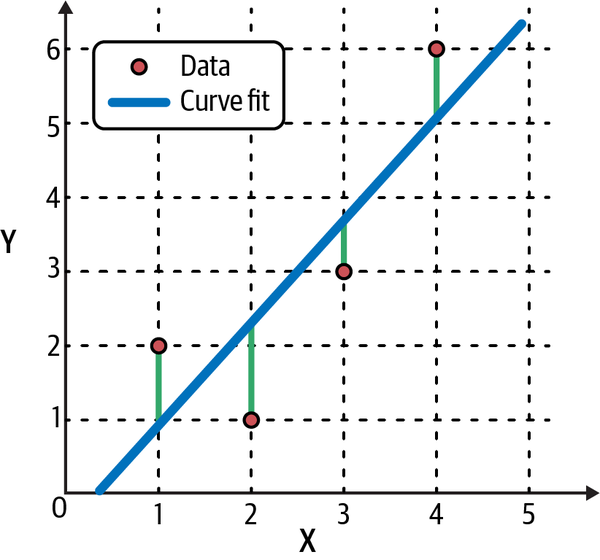
Figure 7-1. The line of best fit of a linear regression model. The residuals are the vertical lines between the observed data and the fitted line.1
As shown in Figure 7-1, the target (Y) of a simple linear regression model has only one feature (X) and is expressed as:
- Y = a + b × X + e, where a and b are constants to be learned from training data by minimizing the residual, e = Y − Y′.
A multiple linear regression model uses a linear combination of more than one feature for predicting the target. The general form of linear regression is expressed as:
- Y = b0 + b1 × X1 + b2 × X2 + …+ bn × Xn + e, where b0 − bn are constants to be learned from training data by minimizing the residual, e = Y − Y′.
It is important to note that in a linear model, it is the coefficients (b0 – bn) that have to be linear, and not the features. Recall from Chapter 4 that a financial analyst, relying on modern portfolio theory and the practice of the frequentist statistical approach, incorrectly assumes that there is an underlying, time-invariant, stochastic process generating the price data of an asset such as a stock.
Market Model
This stochastic process can be modeled as an MM, which is basically a simple linear regression model of the realized excess returns of the stock (target) regressed on the realized excess returns of the overall market (feature), as formulated here:
- (R − F) = a + b (M − F) + e (Equation 7.1)
-
Y = (R – F) is the target, X = (M − F) is the feature.
-
R is the realized return of the stock.
-
F is the return on a risk-free asset (such as the 10-year US Treasury note).
-
M is the realized return of a market portfolio (such as the S&P 500 index).
-
a (alpha) is the expected stock-specific return.
-
b (beta) is the level of systematic risk exposure to the market.
-
e (residual) is the unexpected stock-specific return.
Even though the alpha and beta parameters of this underlying random process may be unknown or unknowable, the analyst is made to believe that these parameters are constant and have “true” values. The assumed time-invariant nature of this stochastic process implies that model parameters can be estimated from any random sample of price data of the various securities involved over a reasonably long amount of time. This implicit assumption is known as the stationary ergodic condition. It is the randomness of sample-to-sample data that creates aleatory uncertainty in the estimates of the true, fixed parameters, according to frequentists. The aleatory uncertainty of the parameters is captured by the residual, e = (Y – Y′).
Model Assumptions
Many analysts are generally not aware that in order to make sound inferences about the model parameters, they have to make further assumptions about the residuals based on the Gauss-Markov theorem, namely:
-
The residuals are independent and identically distributed.
-
The expected mean of the residuals is zero.
-
The variance of the residuals is constant and finite.
Learning Parameters Using MLE
If the analyst assumes that the residuals are normally distributed, then it can be shown with basic calculus that the maximum likelihood estimate (MLE) for both parameters, alpha and beta, have the same values as those obtained using the OLS algorithm we learned in high school and applied in Chapter 4 using the Statsmodels library. This is because both algorithms are minimizing the mean squared error or the expected value of the square of the residuals E[(Y − Y′)2)]. However, the MLE algorithm is preferred over the OLS algorithm because it can be applied to many different types of likelihood functions.2
It is common knowledge that while financial data are abundant, they have very low signal-to-noise ratios. One of the biggest risks in financial ML is that of variance or overfitting of data. When the model is trained on data, the algorithm learns the noise instead of the signal. This results in model parameter estimates that vary wildly from sample to sample. Consequently, the model performs poorly in out-of-sample testing.
In multiple linear regression, overfitting of the data also occurs because the model might have highly correlated features. This is also called multicollinearity and is common in the financial and business world, where most features are interconnected, especially in times of financial distress.
Conventional statisticians have developed two ad hoc methods called regularizations to reduce this overfitting of noisy data by creating a penalty term in the optimization algorithm for reducing the impact of any one parameter. Never mind that this is the antithesis of the frequentist decree of letting “only the data speak for themselves.”
There are two types of regularization methods that penalize model complexity:
- Lasso or L1 regularization
- Penalizes the sum of the absolute values of the parameters. In Lasso regression, many of the parameters are shrunk to zero. Lasso is also used to eliminate correlated features and improve the interpretation of complex models.
- Ridge or L2 regularization
- Penalizes the sum of the coefficients squared of the parameters. In ridge regression, all parameters are shrunk to near zero, which reduces the impact of any one feature on the target variable.
In other words, instead of “only letting the data speak for themselves,” L2 regularization stifles all the voices, while L1 regularization silences many of them. Of course, models are regularized to make them useful in finance and investing, where data are extremely noisy, and the following Fisher’s dictum results in regression models failing abysmally and losing money.
Quantifying Parameter Uncertainty with Confidence Intervals
After estimating the model parameters from training data, the analyst computes the confidence intervals for alpha and beta to quantify their aleatory uncertainty. Most analysts are unaware about the three types of errors of using confidence intervals and don’t understand their flaws, as was discussed in Chapter 4. If they did, they would never use confidence intervals in financial analysis except in special cases when the central limit theorem applies.
Predicting and Simulating Model Outputs
Now that the linear model has been built, it is tested on unseen data to evaluate its usefulness for estimating and predicting. The same type of scoring algorithms that are used to evaluate the performance of the model on training data are used on testing data to compute its usefulness. However, to simulate data, the analyst will have to set up a separate Monte Carlo simulation (MCS) model, as discussed in Chapter 3. This is because MLE models are not generative models. They do not learn the underlying statistical structure of the data and so are unable to simulate data.
Probabilistic Linear Ensembles
In MLE modeling, the financial analyst tries to build models that are expected to emulate a “true” model that is supposedly optimal, elegant, and eternal. In probabilistic modeling, the financial analyst is freed from such ideological burdens. They don’t have to apologize for their financial models being approximate, messy, and transient because they merely reflect mathematical and market realities. We know that all models are wrong regardless of whether they are treated as prophetic or pathetic. We only evaluate them on their usefulness in achieving our financial goals.
The financial analyst using the probabilistic framework not only applies the inverse probability rule, but also inverts the MLE modeling paradigm. Spurning ideological dictums of orthodox statistics in favor of common sense and the principles of the scientific method, they invert the conventional treatment of data and parameters:
-
Training data of excess returns, such as Y = (R − F) and X = (M − F), are treated as constants because their values have already been realized and recorded and will never change. That is the epitome of what a constant means.
-
Model parameters, such as alpha (a), beta (b), and the residual (e), are treated as variables with probability distributions since their values are unknown and uncertain. Financial model parameters have aleatory, epistemic, and ontological uncertainty. Their estimates keep changing depending on the sample used, assumptions applied, and the time period involved. That is the quintessence of what a variable means.
The analyst understands that the search for any “true” constant parameter value of a financial model is a fool’s errand. This is because the dynamic randomness of markets and their participants ensure that probability distributions are never stationary ergodic. These analysts are painfully aware that creative, free-willed, emotional human beings make a mockery of theoretical, MLE-based “absolutist” financial models almost every day. The frequentist claim that financial model parameters have “true” values is simply unscientific, ideological drivel.
We will use the probabilistic framework to explicitly state our assumptions and assign specific probability distributions to all the terms of the probabilistic framework so far discussed. Each probability distribution has additional parameters that will have to be estimated by the analyst. The analyst will have to specify the reasons for their choices. If the models fail during the testing phase, the analysts will change any and all probability distributions, including their parameters. All financial models are developed based on the most fundamental of heuristic techniques: trial and error.
In a probabilistic framework, we apply the inverse probability rule to estimate our model parameters, as developed in Chapter 5. After we have designed our model, we will develop it in Python using the PyMC library. Based on the terms defined for the MM, the probabilistic linear ensemble (PLE) is formulated as:
- P(a, b, e| X, Y) = P(Y| a, b, e, X) P(a, b, e) / P(Y|X) where
-
Y = a + b × X + e, as expressed in the MLE linear model, but without its explicit or implicit assumptions. These will be specified explicitly in the PLE.
-
P(a, b, e) are the prior probabilities of all model parameters before observing the training data (X, Y).
-
P(Y| a, b, e, X) is the likelihood of observing the target training data Y given the parameters a, b, e, and feature training data X.
-
P(Y|X) is the marginal likelihood of observing the training values of target Y given the training values of feature X averaged over all possible prior values of the parameters (a, b, e).
-
P(a, b, e| X, Y) is the posterior probabilities of the parameters a, b, e given the training data (X,Y).
We now discuss each component of the PLE model in more detail.
Prior Probability Distributions P(a, b, e)
Before the analyst sees any training data (X,Y), they may specify the prior probability distributions of the PLE parameters (a, b, e) and quantify their epistemic uncertainty. All prior distributions are assumed to be independent of one another. These prior distributions may be based on personal, institutional, experiential, or common knowledge. If the analyst does not have any prior knowledge about the parameters, they can express their ignorance with uniform distributions that consider each value between the upper and lower limits equally likely. Remember that having bounds of 0 and 1 should be avoided unless you are absolutely certain that a parameter can take these values. The main objective is to specify one of the most important model assumptions explicitly and quantitatively.
Given the tendency of models to overfit noisy financial data that don’t have any persistent structural unity, the analyst is aware that it is foolish to follow the orthodox dictum of “only letting the data speak for themselves.” The ad hoc use of regularization methods in MLE models to manage this overfitting risk are merely prior probability distributions in disguise. It can be shown mathematically that L1 regularization is equivalent to using a Laplacian prior, and L2 regularization is equivalent to using a Gaussian prior.3
The analyst systematically follows the probabilistic framework and explicitly quantifies their knowledge, or ignorance, about the model parameters with prior probability distributions. This makes the model transparent so it can be changed and critiqued by anyone, especially the portfolio manager. For instance, the analyst could assume that:
-
alpha is normally distributed: a ~Normal()
-
beta is normally distributed: b ~Normal()
-
Residual is Half-Student’s t-distributed: e ~HalfStudentT()
Likelihood Function P(Y| a, b, e, X)
After the analyst observes the training data (X,Y), they need to formulate a likelihood function that best fits that data and quantifies the aleatory uncertainty of the model parameters (a, b, e). This is the same likelihood function that was used in the MLE linear model. In standard linear regression, the likelihood function for the residuals (e) is assumed to be a Gaussian or normal distribution. However, instead of using a normal probability distribution, the analyst uses Student’s t-distribution to model the financial realities of fat-tailed asset price returns. Also, if the likelihood function can accommodate outliers as well as the Student’s t-distribution does, the linear regression is termed a robust linear regression.
Student’s t-distribution is a family of distributions that can approximate a range of other probability distributions based on its degrees of freedom parameter, v, which is a real number that can range from 0 to infinity. Student’s t-distributions are fat-tailed for lower values of v and get more normally distributed as v gets larger. It is important to note that for:
-
v ≤ 1, t-distributions have no defined mean and variance
-
1 < v ≤ 2, t-distributions have a defined mean but no defined variance
-
v > 30, t-distributions are approximately normally distributed
Say the analyst assigns a Student’s t-distribution with v = 6 to the likelihood function. Why v = 6? Financial research and practice has shown that this t-distribution does a good job of describing the fat-tailed stock price returns. So we are applying prior common knowledge to the choice of the likelihood function. The specific likelihood function can be expressed mathematically as:
-
Y ~StudentT(u, e, v = 6) where u = a + b × X and (a, b, e) are as defined by their prior probability distributions
Marginal Likelihood Function P(Y|X)
This is the hardest function to compute given it is averaging the likelihood functions over all the model’s parameters. The complexity increases as the types of probability distributions and number of parameters increase. As was mentioned earlier, we need groundbreaking algorithms to approximate this function numerically.
Posterior Probability Distributions P(a, b, e| X, Y)
Now that we have our model specified, we can compute the posterior probabilities for all our model’s parameters (a, b, e) given our training data (X,Y). To recap, our model is specified as follows:
-
Y ~StudentT(u, e, v = 6)
-
u = a + b × X
-
a ~Normal(), b ~Normal(), e ~HalfStudentT()
-
X,Y are training data pairs in a sample time period that reflect the current market conditions.
Model parameters, their probability distributions, and their relationships are displayed in Figure 7-2.
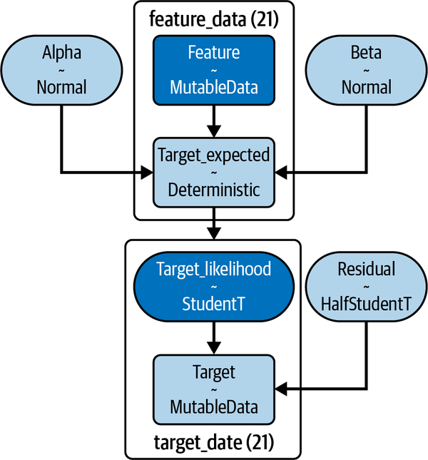
Figure 7-2. Probabilistic market model showing prior distributions used for parameters and the likelihood function used to fit training data
Because of the complexity of any realistic model, especially the marginal likelihood function, we can only approximate the posterior distributions of each of its parameters. PyMC uses the appropriate state-of-the-art MCMC algorithm to simulate the posterior distribution by sampling from it as discussed in Chapter 6. We then use the ArviZ library to explore these samples, enabling us to draw inferences and make predictions from them.
Assembling PLEs with PyMC and ArviZ
Let’s now build our PLE in Python by leveraging its extensive ecosystem of powerful libraries. In addition to the standard Python stack of NumPy, pandas, and Matplotlib, we will also be using PyMC, ArviZ, and Xarray libraries. As mentioned earlier, PyMC is the most popular probabilistic machine learning library in Python. ArviZ is a probabilistic language-agnostic tool for analyzing and visualizing probabilistic ensembles. It converts inference data of probabilistic ensembles into Xarray objects, which are labeled, multidimensional arrays. You can search the web for links to the relevant documentation of the previously mentioned libraries.
Building an ensemble of any kind requires a systematic process, and our PLE is no exception. We will follow the high-level ensemble-building process outlined in Figure 7-3. Each phase and its constituent parts will be explained along with the relevant code. It is important to note that even though we will go through our ensemble building process sequentially, this is an iterative, nonlinear process in practice. For instance, you could easily go back and forth from the training phase to the analyze features and target data phase. With that nonlinearity in mind, let’s go to the first phase.
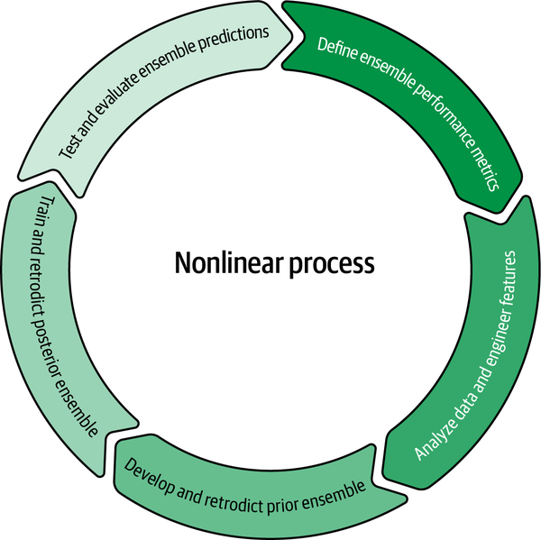
Figure 7-3. High-level process for assembling probabilistic learning ensembles
Define Ensemble Performance Metrics
Our financial objectives and activities should drive the effort of building our PLE. Consequently, this influences the metrics we use to evaluate its performance. Our financial tasks are generally to estimate the parameters of a financial model or to forecast its outputs or both. As you know by now, probabilistic machine learning systems are ideally suited to both these tasks because they do inverse propagation and forward propagation seamlessly. More importantly, these generative ensembles direct us to consider the aleatory and epistemic uncertainties of the problem we are addressing and its possible solutions.
Financial activities
Plausible estimates of the regression parameters alpha and beta in Equation 7.1 are required for several financial activities that are practiced in the industry:
- Jensen’s alpha
- By regressing the returns of a fund against the returns of its benchmark portfolio, investors evaluate the skill of the fund’s manager by estimating the regression’s alpha parameter. This metric is known as Jensen’s alpha in the industry.
- Market neutral strategies
- Alpha can also be viewed as the asset-specific expected return regardless of the movements of the market. If a fund manager finds this return significantly attractive, they can try to isolate it and capture it by hedging out the asset’s exposure to market movements. This also involves estimating the asset’s beta, or sensitivity to the market. The portfolio consisting of the asset and the hedge becomes indifferent or neutral to the vagaries of the market.
- Cross-hedging
- By assuming constant variance of the residuals in Equation 7.1, the beta parameter can also be shown mathematically to correlate the volatility of one asset (Y) with the volatility of another related asset (X). Cross-hedging programs in corporate treasury departments use this beta-related correlation to hedge a commodity required by their company, say jet fuel, with another related commodity, such as oil. Treasury departments buy or sell financial instruments, such as futures, in the open market to hedge their input costs.
- Cost of equity capital
- Corporate financial analysts estimate the cost of their company’s equity capital by estimating the realized return, R, in the regression Equation 7.1. This is supposedly the expected return on their stock that their public shareholders are demanding. Many analysts still use their stock’s CAPM model and estimate R by making alpha = 0 in Equation 7.1.
In this chapter, we will focus on estimating Apple’s equity price returns by using its MM, and not its CAPM, for the reasons detailed in Chapter 4. We will estimate the posterior probability distribution of Apple’s excess returns (R - F) given the current market regime. The generative linear ensemble can be applied to all the financial activities discussed earlier.
Objective function
A rule that is formulated to measure the performance of a model or ensemble is called an objective function. This function generally measures the difference between the ensemble’s estimates or predictions compared with the corresponding realized or observed values. Common objective functions that measure the difference between predicted and observed values in machine learning regression models are mean squared error (MSE) and median absolute errors (MAE). The choice of an objective function depends on the business problem we are trying to solve. An objective function that reduces losses/costs is called a loss/cost function.
Another regression objective function is R-squared. In frequentist statistics, it is defined as the variance of the predicted values divided by the total variance of the data. Note that R-squared can be interpreted mathematically as a standardized MSE objective function that needs to be maximized:
- R-squared(Y) = 1 – MSE(Y)/Var(Y)
Since we are dealing with aleatory and epistemic uncertainties in our probabilistic models, this R-squared formula has to be modified so that its value does not exceed 1. The probabilistic version of R-squared is modified to equal the variance of the predicted values divided by the variance of predicted values plus the expected variance of the errors. It can be interpreted as a variance decomposition.4 We will call this version of the R-squared objective function probabilistic R-squared.
Performance metrics
As mentioned earlier, financial data are very noisy, which implies that we need to be realistic about the performance metrics we establish for each development phase. At a minimum, we want our model to do better than random guessing, i.e., we want performance scores greater than 50%. We would like our PLE to meet or exceed the following performance metrics:
-
Probabilistic R-squared prior score > 55%
-
Probabilistic R-squared training score > 60%
-
Probabilistic R-squared test score > 65%
-
Highest-density intervals (HDIs): 90% HDI to include almost all training and test data (HDI will be explained shortly)
Keep in mind that all these metrics will be based on personal and organization preferences and are imperfect, as are the models used to produce them. It requires judgment and domain expertise. Regardless, we will use these metrics as another input to help us to evaluate our PLE, critique it, and revise it. In practice, we revise our PLE until we are confident that it will give us a high enough positive expected value in the financial activity we want to apply it to. Only then do we deploy our PLE out of the lab.
Analyze Data and Engineer Features
We have already done data analysis of the target and features in Chapter 4 and in rewriting Equation 7.1.
Data exploration
In general, in this phase you would define your target of interest, such as predicting asset price returns or estimating volatility. These target variables are real valued numbers and are termed as regression targets. Alternatively, a target of interest could also be classification of a company’s creditworthiness based on predictions of whether it will default or not. These are classification targets that take on discrete numbers like 0 or 1.
You would then identify various sources of data that will enable you to analyze your target and features in sufficient detail. Data sources can be expensive, and you will have to figure out how to get them in a cost-effective manner. Cleaning and processing data from various sources is generally quite time-consuming.
Feature engineering
Recall that a feature is some representation of data that serves as an independent variable enabling inference or prediction of a model’s target variable. Feature engineering is the practice of selecting, designing, and developing a useful set of features that work together to enable reliable inferences or predictions of the target variable(s) in out-of-sample data.
To predict a target variable, such as price returns, a model can have many different types of features. Here are examples of various types of features:
- Fundamental
- Company sales, interest rates, exchange rates, GDP growth rate
- Technical
- Momentum indicators, fund flows, liquidity
- Sentiment
- Consumer sentiment, investor sentiment
- Other
- Proprietary mathematical or statistical indicators
After you have selected and developed a possible set of features, it is generally a good idea to use relative changes in feature levels, rather than absolute levels, as inputs into your features’ dataframe. This reduces the serial autocorrelation endemic in financial time series. Serial correlation occurs when a variable is correlated with past values of itself over time. Traders and investors are generally interested in understanding if a good or bad condition is getting better or worse. So market participants are continually reacting to relative changes in levels in terms of percentages or differences.
If we have more than one feature, we need to check if some of them are highly correlated with one another. Recall that this issue is called multicollinearity. Highly correlated features can unduly amplify the same signal in data, leading to invalid inferences and predictions. Ideally, there should be zero correlation or no multicollinearity among features. Unfortunately, that almost never happens in practice. Coming up with a threshold variance above which you would remove redundant features is a judgment call based on the business context.
Feature engineering is critical to the performance of all ML systems. It requires domain expertise, judgment, experience, common sense, and a lot of trial and error. These are the qualities that enable human intelligence to distinguish correlation from causation, which AI-enabled agents cannot do to this day.
We are going to keep our feature engineering simple in this primer and leverage a vast body of financial knowledge and experience on market models. Our PLE has a single feature: the market as represented by the S&P 500 index.
Data analysis
PLEs demonstrate their strengths when we have small datasets, such that a weak or flat prior is not overwhelmed by the likelihood function. Here we will look at 31 days of data in the last two months of last year, from 11/15/2022 to 12/31/22. This period covers two Federal Reserve meetings and was exceptionally volatile. We will train our PLE on the first 21 days of data and test it on the last 10 days of data. This is called the time series split method of cross-validation. Because financial time series have strong serial correlation, we cannot use the standard cross-validation method, since it assumes that each data sample is independent and identically distributed.
Let’s actually download price data for Apple Inc., S&P 500, and the 10-year treasury note, and compute the daily price returns as we did for our linear MM in Chapter 4:
# Import standard Python libraries.importnumpyasnpimportpandasaspdfromdatetimeimportdatetimeimportxarrayasxrimportmatplotlib.pyplotasplt# Install and import PyMC and Arviz libraries.!pipinstallpymc-qimportpymcaspmimportarvizasazaz.style.use('arviz-darkgrid')# Install and import Yahoo Finance web scraper.!pipinstallyfinance-qimportyfinanceasyf# Fix random seed so that numerical results can be reproduced.np.random.seed(101)# Import financial data.start=datetime(2022,11,15)end=datetime(2022,12,31)# S&P 500 index is a proxy for the market factor.market=yf.Ticker('SPY').history(start=start,end=end)# Ticker symbol for Apple, the largest company in the world# by market capitalization.stock=yf.Ticker('AAPL').history(start=start,end=end)# 10 year US treasury note is the proxy for risk free rate.riskfree_rate=yf.Ticker('^TNX').history(start=start,end=end)# Create a dataframe to hold the daily returns of securities.daily_returns=pd.DataFrame()# Compute daily percentage returns based on closing prices for Apple and# S&P 500 index.daily_returns['market']=market['Close'].pct_change(1)*100daily_returns['stock']=stock['Close'].pct_change(1)*100# Compounded daily risk free rate based on 360 days for the calendar year# used in the bond market.daily_returns['riskfree']=(1+riskfree_rate['Close'])**(1/360)-1# Check for missing data in the dataframe.market.index.difference(riskfree_rate.index)# Fill rows with previous day's risk-free rate since# daily rates are generally stable.daily_returns=daily_returns.ffill()# Drop NaNs in first row because of percentage calculations# are based on previous day's closing price.daily_returns=daily_returns.dropna()# Check dataframe for null values.daily_returns.isnull().sum()# Check first five rows of dataframe.daily_returns.head()# Daily excess returns of AAPL are returns in excess of# the daily risk free rate.y=daily_returns['stock']-daily_returns['riskfree']# Daily excess returns of the market are returns in excess of# the daily risk free rate.x=daily_returns['market']-daily_returns['riskfree']# Plot the excess returns of Apple and S&P 500.plt.scatter(x,y)plt.ylabel('Excess returns of Apple'),plt.xlabel('Excess returns of S&P 500');# Plot histogram of Apple's excess returns during the period.plt.hist(y,density=True,color='blue')plt.ylabel('Probability density'),plt.xlabel('Excess returns of Apple');# Analyze daily returns of all securities.daily_returns.describe()# Split time series sequentially because of serial correlation# in financial data.test_size=10x_train=x[:-test_size]y_train=y[:-test_size]x_test=x[-test_size:]y_test=y[-test_size:]
Develop and Retrodict Prior Ensemble
Let’s start developing our PLE using the PyMC library. At this point, we explicitly state the assumptions of our ensemble in the prior probability distributions of the parameters and the likelihood function. This also includes our hypothesis about the functional form of the underlying data-generating process, i.e., linear with some noise.
After that, we check to see if the ensemble’s prior predictive distribution generates data that is plausible and may have occurred in the past, and are now in our training data sample. A prediction of a past event is called retrodiction and is used as a model check, before and after it is trained. If the data generated by the prior ensemble are implausible, because they don’t fall within our highest density interval, we revise all of our model assumptions.
Specify distributions and their parameters
We incorporate our prior knowledge into the ensemble by specifying the prior probability distributions of its parameters, P(a), P(b), and P(e). After that, we specify the likelihood of observing our data given the parameters, P(D | a, b, e).
In the following Python code block, we have chosen a Student’s t-distribution with nu = 6 for the likelihood function of our ensemble. Of course, we could also add nu as another unknown parameter that needs to be inferred. However, that would merely increase the complexity without adding much in terms of increasing your understanding of the development process.
# Create a probabilistic model by instantiating the PyMC model class.model=pm.Model()# The with statement creates a context manager for the model object.# All variables and constants inside the with-block are part of the model.withmodel:# Define the prior probability distributions of the model's parameters.# Use prior domain knowledge.# Alpha quantifies the idiosyncratic, daily excess return of Apple# unaffected by market movements.# Assume that alpha is normally distributed. The values of mu and# sigma are based on previous data analysis and trial and error.alpha=pm.Normal('alpha',mu=0.02,sigma=0.10)# Beta quantifies the sensitivity of Apple to the movements# of the market/S&P 500.# Assume that beta is normally distributed. The values of mu and# sigma are based on previous data analysis and trial and error.beta=pm.Normal('beta',mu=1.2,sigma=0.15)# Residual quantifies the unexpected returns of Apple# i.e returns not predicted by the linear model.# Assume residuals are Half Student's t-distribution with nu=6.# Value of nu=6 is based on research studies and trial and error.residual=pm.HalfStudentT('residual',sigma=0.20,nu=6)# Mutatable data containers are used so that we can swap out# training data for test data later.feature=pm.MutableData('feature',x_train,dims='feature_data')target=pm.MutableData('target',y_train,dims='target_data')# Expected daily excess returns of Apple are approximately# linearly related to daily excess returns of S&P 500.# The function specifies the linear model and the expected return.# It creates a deterministic variable in the trace object.target_expected=pm.Deterministic('target_expected',alpha+beta*feature,dims='feature_data')# Assign the training data sample to the likelihood function.# Daily excess stock price returns are assumed to be T-distributed, nu=6.target_likelihood=pm.StudentT('target_likelihood',mu=target_expected,sigma=residual,nu=6,observed=target,dims='target_data')
Figure 7-2 was generated by the graphviz method shown in the following code:
# Use the graphviz method to visualize the probabilistic model's data,# parameters, distributions and dependenciespm.model_to_graphviz(model)
Sample distributions and simulate data
Before we train our model, we should check the usefulness of the assumptions of our prior ensemble. The goal is to make sure that the ensemble is good enough for the training phase. This is done by conducting what is called a prior predictive check. We use the ensemble’s prior predictive distribution to simulate a data distribution that may have been realized in the past. Recall that this is called a retrodiction as opposed to a prediction, which simulates a data distribution that is most likely to occur in the future.
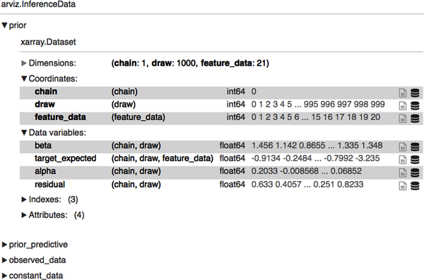
In the following code block, we simulate 21,000 data samples from the prior predictive distribution. We let ArviZ return the InferenceData object so that we can visualize and analyze the generated data samples. Expand the display after the inference object is returned to examine the structure of the various groups. We will need them for analysis and inference:
# Sample from the prior distributions and the likelihood function# to generate prior predictive distribution of the model.# Take 1000 draws from the prior predictive distribution# to simulate (1000*21) target values based on our prior assumptions.idata=pm.sample_prior_predictive(samples=1000,model=model,return_inferencedata=True,random_seed=101)# PyMC/Arviz returns an xarray - a labeled, multidimensional array# containing inference data samples structured into groups. Note the# dimensions of the prior predictive group to see how we got (1*1000*21)# simulated target data of the prior predictive distribution.idata
Let’s plot the marginal prior distributions of each parameter before we conduct prior predictive checks. Note that a kernel density estimate is a smoothed-out histogram of a continuous variable:
# Subplots on the left show the kernel density estimates (KDE) of# the marginal prior probability distributions of model parameters# from the 1000 samples drawn. Subplots on the right show the parameter# values from a single Markov chain that were sampled sequentially# by the NUTS sampler, the default regression sampler.az.plot_trace(idata.prior,kind='trace',var_names=['alpha','beta','residual'],legend=True);
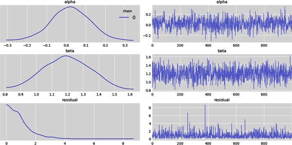
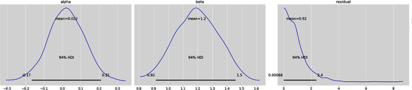
# Plot the marginal prior distributions of each parameter with 94%# highest density intervals (HDI).# Note the residual subplot shows the majority of probability density function# within 3 percentage points and the rest extending out into a long tail.# In Arviz, there is no method to plot the prior marginal distributions but we# can hack the plot posterior method and use the prior group instead.az.plot_posterior(idata.prior,var_names=['alpha','beta','residual'],round_to=2);
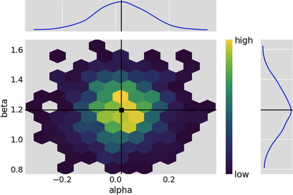
# Plot the joint prior probability distribution of alpha and beta with their# respective means and marginal distributions on the side.# Hexabin plot below shows little or no linear correlation with the high# concentration areas in the heat map forming a cloud.az.plot_pair(idata.prior,var_names=['alpha','beta'],kind='hexbin',marginals=True,point_estimate='mean',colorbar=True);
Let’s create a prior ensemble of 1000 regression lines, one for each value of the ensemble’s parameters (a, b) sampled from its prior distributions, and plot the epistemic uncertainty around the prior mean of the untrained linear ensemble. We also use the prior predictive distribution of the ensemble to simulate data. This displays the epistemic and aleatory uncertainties of the data distributions. Note that the training data is plotted to give us some context and a baseline for the ensemble’s retrodictions:
# Plot the retrodictions of prior predictive ensemble.# Retrieve feature and target training data from the constant_data group.# Feature is now an Xarray instead of a panda's series,# a requirement for ArviZ data analysis.feature_train=idata.constant_data['feature']target_train=idata.constant_data['target']# Generate 1000 linear regression lines based on 1000 draws from one# Markov chain of the prior distributions of alpha and beta.# Prior target values are in 1000 arrays with each array having 21 samples,# the same number of samples as our training data set.prior_target=idata.prior["alpha"]+idata.prior["beta"]*feature_train# Prior_predictive is the data generating distribution of the untrained ensemble.prior_predictive=idata.prior_predictive['target_likelihood']# Create figure of subplotsfig,ax=plt.subplots()# Plot epistemic and aleatory uncertainties of untrained# ensemble's retrodictions.az.plot_lm(idata=idata,x=feature_train,y=target_train,num_samples=1000,y_model=prior_target,y_hat=prior_predictive,axes=ax)#Label the figure.ax.set_xlabel("Excess returns of S&P500")ax.set_ylabel("Excess returns of Apple")ax.set_title("Retrodictions of untrained linear ensemble")ax.legend(loc='upper left');
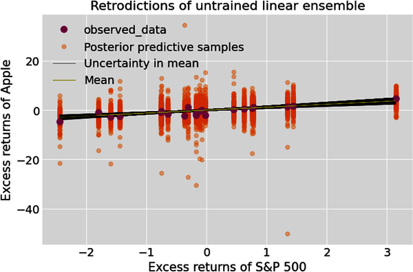
It is very important to observe that the linear ensemble’s epistemic uncertainty increases as we move away from the center of the plot. Confessions of ignorance is what we are seeking in any model: it should become increasingly unsure about its expected values as it moves into regions where it has no data and must extrapolate. Our ensemble knows its limitations.
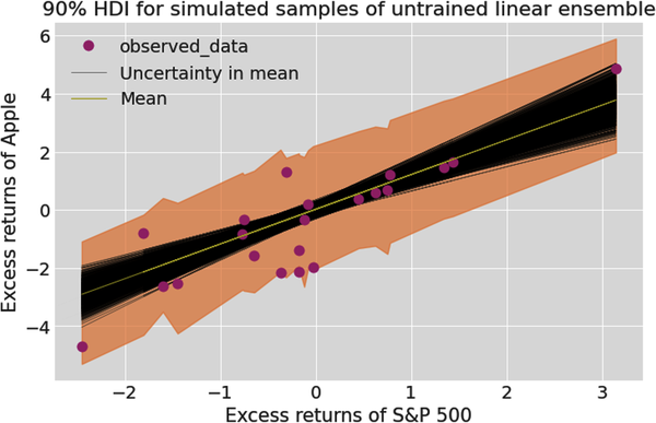
This is seen more clearly in the next plot where we generate and distribute the prior predictive data samples into a 90% high-density interval (HDI) and then conduct a prior predictive check:
# Plot 90% HDI of untrained ensemble.# This will show the aleatory (data related) and epistemic# (parameter related) uncertainty of model output before it is trained.# Create figure of subplots.fig,ax=plt.subplots()# Plot the ensemble of 1000 regression lines to show the# epistemic uncertainty around the mean regression line.az.plot_lm(idata=idata,x=feature_train,y=target_train,num_samples=1000,y_model=prior_target,axes=ax)# Plot the prior predictive data within the 90% HDI band to# show both epistemic and aleatory uncertainties.az.plot_hdi(feature_train,prior_predictive,hdi_prob=0.90,smooth=False)# Label figure.ax.set_xlabel("Excess returns of S&P 500")ax.set_ylabel("Excess returns of Apple")ax.set_title("90% HDI for simulated samples of untrained linear ensemble")ax.legend();
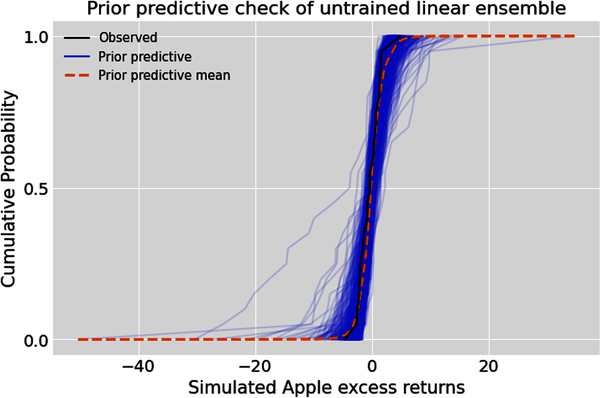
# Conduct a prior predictive check of the untrained linear ensemble.# Create figure of subplots.fig,ax=plt.subplots()# Plot the prior predictive checkaz.plot_ppc(idata,group='prior',kind='cumulative',num_pp_samples=1000,alpha=0.1,ax=ax)# Label the figure.ax.set_xlabel("Simulated Apple excess returns")ax.set_ylabel("Cumulative Probability")ax.set_title("Prior predictive check of untrained linear ensemble");
Evaluate and revise untrained model
Specifying a probabilistic model is never easy, and requires many revisions. Let’s use qualitative and quantitative prior predictive checks to see if our prior model is plausible and ready for training. From the recent plots, we can see that our ensemble has simulated all the training data within the 90% HDI band. However, the prior predictive check shows some low probability, extreme returns that have not occurred in the recent past. Let’s now compute the probabilistic R-squared measure to evaluate the ensemble’s retrodictions before it has been trained:
# Evaluate untrained ensemble's retrodictions by comparing simulated# data with training data.# Extract target values of our training data.target_actual=target_train.values# Sample the prior predictive distribution to simulate# expected target training values.target_predicted=idata.prior_predictive.stack(sample=("chain","draw"))['target_likelihood'].values.T# Use the probabilistic R-squared metric.prior_score=az.r2_score(target_actual,target_predicted)prior_score.round(2)
The probabilistic R-squared metric of the prior ensemble is 61%, with a standard deviation of 10%. This exceeds our performance benchmark of 55% for the prior model.
Please note that this performance is a result of many revisions to the prior model I made by changing the values of the various parameters of the prior distributions. I also experimented with different distributions, including a uniform prior for the alpha parameter. All the prior scores were greater than 55%, and the one you see here is closer to the median score. Feel free to make your own revisions to the prior model until you are satisfied that your ensemble is plausible and ready to be trained by in-sample data.
Train and Retrodict Posterior Model
We now have an ensemble that is ready to be trained, and we are confident it reflects our prior knowledge, including the epistemic uncertainty of its parameters and the aleatory uncertainty of the data it might generate. Let’s train it with actual in-sample data our ensemble has been anticipating by computing the posterior distribution.
Train and sample posterior
We execute the default sampler of PyMC, the Hamiltonian Monte Carlo (HMC) algorithm, a second-generation MCMC algorithm. PyMC directs HMC to generate dependent random samples from the joint posterior distribution of all the parameters:
# Draw 1000 samples from two Markov chains resulting in 2000 values of each# parameter to analyze the joint posterior distribution.# Check for any divergences in the progress bar. We want 0 divergences for a# reliable sampling of the posterior distribution.idata.extend(pm.sample(draws=1000,chains=2,model=model,random_seed=101))

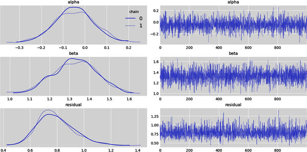
Evaluating the quality of the MCMC sampling is an advanced topic and will not be covered in this primer. Since we have no divergences in the Markov chains, let’s analyze the marginal distribution of each parameter and make inferences about each of them:
# Subplots on the left show the kernel density estimates (KDE)# of the marginal posterior probability distributions of each parameter.# Subplots on the right show the parameter values# that were sampled sequentially in two chains by the NUTS samplerwithmodel:az.plot_trace(idata.posterior,kind='trace',var_names=['alpha','beta','residual'],legend=True)
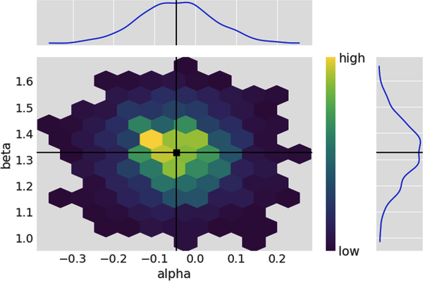
# Plot the joint posterior probability distribution of alpha and beta# with their respective means and marginal distributions on the side.# Hexabin plot below shows little or no linear correlation with the# high concentration areas in the heat map forming a cloud.az.plot_pair(idata.posterior,var_names=['alpha','beta'],kind='hexbin',marginals=True,point_estimate='mean',colorbar=True);
We can summarize the posterior distributions in a pandas DataFrame as follows:
# Examine sample statistics of each parameter's posterior marginal distribution,# including it's 94% highest density interval (HDI).display(az.summary(idata,kind='stats',var_names=['alpha','beta','residual'],round_to=2,hdi_prob=0.94))
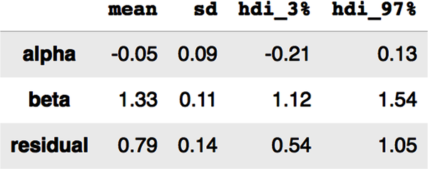
This statistical summary gives you the mean, standard deviation, and a 94% credible interval for all our parameters. Note that the 94% credible intervals are computed as the differences between the highest density intervals (HDI): hdi_97% – hdi_3% = hdi_94%.
Unlike the shenanigans of frequentist confidence intervals discussed in Chapter 4, a credible interval is exactly what a confidence interval pretends to be but is not. Credible intervals are a postdata methodology for making valid statistical inferences from a single experiment. This is exactly what we want as researchers, scientists, and practitioners in any field. For instance, the 94% credible interval for beta in the summary table means the following:
-
There is a 94% probability that beta is in the specific interval [1.12 and 1.55]. It is as simple as that. Unlike confidence intervals, we don’t have to deal with some warped definition that defies any semblance of common sense to interpret credible intervals.
-
There are no assumptions of asymptotic normality of any distribution.
-
There are no underhanded invocations to the central limit theorem.
-
Beta is not a point estimate with only aleatory uncertainty.
-
We are ignorant of the exact value of beta. It is highly unlikely that we will ever know the exact values of any model parameter for any realistic scenario in the social and economic sciences.
-
Parameters like beta are better interpreted as probability distributions with both aleatory and epistemic uncertainties.
-
It is much more realistic to model and interpret parameters like beta as unknowable variables rather than as unknowable constants.
It is important to note that credible intervals are not unique within a posterior distribution. Our preferred way is to choose the narrowest interval with the highest probability density within the posterior distribution. Such an interval is also known as the highest-density interval (HDI) and is the method we have been following in this chapter.
You might be wondering why PyMC/ArviZ developers have chosen the default credible interval to be 94%. It is a reminder that there are no physical or socioeconomic laws that dictate that we choose 95% or any other specific percentage. I believe it is a subtle dig at the conventional statistical community for sanctifying the 95% significance level in the social and economic sciences. At any rate, ArviZ provides a method for changing the default interval, as shown in the following code block:
# Change the default highest density interval to 90%az.rcParams['stats.hdi_prob']=0.90
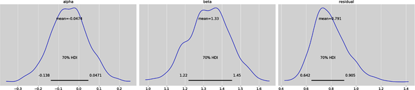
It helps to visualize the posterior distributions of our model parameters for credible intervals with different probabilities. The following plot shows 70% credible intervals for all three parameters:
# Plot the marginal posterior distribution of each parameter displaying# the above statistics but now within a 70% HDIaz.plot_posterior(idata,var_names=['alpha','beta','residual'],hdi_prob=0.70,round_to=3);
More often than not, we have to evaluate point estimates in making our financial and investment decisions. We can estimate how plausible any point estimate of a parameter is based on where it lies within its posterior probability distribution. For instance, if we want to evaluate the point estimate = 1.15 for beta, we can use it as a reference value and compare it to an HDI, as shown in the following code:
# Evaluate a point estimate for a single parameter using its# posterior distribution.az.plot_posterior(idata,'beta',ref_val=1.15,hdi_prob=0.80,point_estimate='mode',round_to=3);
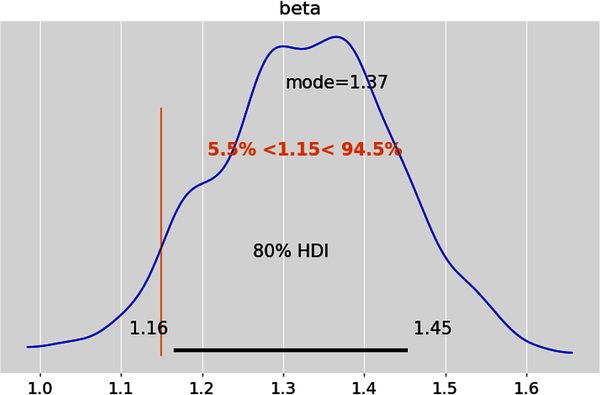
This plot implies that 94.5% of the distribution is above beta = 1.15. Beta = 1.15 is in the left tail of the distribution since only 5.5% of the distribution is below it. Note that the two percentages may not add up to 100% because of rounding errors. So, it is reasonable to conclude that beta = 1.15 is not the best estimate.
Retrodict and simulate training data
We now use the posterior predictive distribution (PPD) to simulate data from the trained ensemble and follow the same steps we did with the ensemble’s prior predictive distribution. This will help us to evaluate how well the ensemble has been trained:
# Draw 1000 samples each from two Markov chains of the# posterior predictive distribution.withmodel:pm.sample_posterior_predictive(idata,extend_inferencedata=True,random_seed=101)
# Generate 2000 linear regression lines based on 1000 draws each from# two chains of the posterior distributions of alpha and beta.# Posterior target values are in 2000 arrays, each with 21 samples,# the same number of samples as our training data set.posterior=idata.posteriorposterior_target=posterior["alpha"]+posterior["beta"]*feature_train# Posterior_predictive is the data generating distribution of the# trained ensemble.posterior_predictive=idata.posterior_predictive['target_likelihood']# Create figure of subplots.fig,ax=plt.subplots()# Plot epistemic and aleatory uncertainties of trained# ensemble's retrodictions.az.plot_lm(idata=idata,x=feature_train,y=target_train,num_samples=2000,y_model=posterior_target,y_hat=posterior_predictive,axes=ax)# Label the figure.ax.set_xlabel("Excess returns of S&P 500")ax.set_ylabel("Excess returns of Apple")ax.set_title("Retrodictions of the trained linear ensemble")ax.legend(loc='upper left');

# Plot 90% HDI of trained ensemble.# This will show the aleatory (data related) and epistemic# (parameter related) uncertainty of model output after it is trained.# Create figure of subplots.fig,ax=plt.subplots()# Plot the ensemble of 2000 regression lines to show the epistemic# uncertainty around the mean regression line.az.plot_lm(idata=idata,x=feature_train,y=target_train,num_samples=1000,y_model=posterior_target,axes=ax)# Plot the posterior predictive data within the 90% HDI band to show both# epistemic and aleatory uncertainties.az.plot_hdi(feature_train,posterior_predictive,hdi_prob=0.90,smooth=False)# Label the figureax.set_xlabel("Excess returns of S&P 500")ax.set_ylabel("Excess returns of Apple")ax.set_title("90% HDI for simulated samples of trained linear ensemble");
# Conduct a posterior predictive check of the trained linear ensemble.# Create a figure of subplots.fig,ax=plt.subplots()# Plot the posterior predictive check.az.plot_ppc(idata,group='posterior',kind='cumulative',num_pp_samples=2000,alpha=0.1,ax=ax)# Label the figure.ax.set_xlabel("Simulated Apple excess returns given training data")ax.set_ylabel("Cumulative Probability")ax.set_title("Posterior predictive check of trained ensemble");
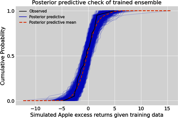
Evaluate and revise trained model
As we did earlier, let’s use qualitative and quantitative checks to see if our posterior model is plausible and ready for testing. The posterior predictive check shows us a range of returns that are more consistent with the recent historical returns of Apple. From its retrodictions, we can see that our ensemble has simulated most of the training data it has been trained on within the 90% HDI band. Let’s now compute the probabilistic R-squared measure to evaluate the trained ensemble’s performance:
# Evaluate trained ensemble's retrodictions by comparing# simulated data with training data.# Get target values of our training datatarget_actual=target_train.values# Sample the posterior predictive distribution# conditioned on training data.target_predicted=idata.posterior_predictive.stack(sample=("chain","draw"))['target_likelihood'].values.T# Compute probabilistic R-squared performance metric.training_score=az.r2_score(target_actual,target_predicted)training_score.round(2)
The probabilistic R-squared metric of the posterior ensemble is 65%, with a standard deviation of 8%. This is a performance improvement compared to that of the untrained ensemble. We can make this comparison because we are using the same dataset to make the performance comparison. It also exceeds the training score benchmark of 60%. Our ensemble is ready for its main test: predictions based on out-of-sample or unseen test data.
Test and Evaluate Ensemble Predictions
We are now confident that our trained ensemble reflects both our prior knowledge and new learnings from the in-sample data that were observed. Moreover, the ensemble has updated its parameter probability distributions in light of the training data, including their epistemic uncertainties. Consequently, the data distributions that the ensemble will generate have also been updated, including their aleatory uncertainties.
The various steps that led us here are all necessary but not sufficient for us to decide if we are going to commit hard-earned capital to the predictions of our ensemble. One of the most important tests for any ML system is how well it performs on previously unseen, out-of-sample test data.
Swap data and resample posterior predictive distribution
PyMC provides mutable data containers that enable the swapping of training data for test data without any other changes to the ensemble. We now have to resample the posterior predictive distribution with the new test data for our target and features.
# Now we use our trained model to make predictions based on test data.# This is the reason we created mutable data containers earlier.withmodel:#Swap feature and target training data for their respective test data.pm.set_data({'feature':x_test,'target':y_test})#Create two new inference groups, predictions and predictions_constant_data#for making predictions based on features in the test data.pm.sample_posterior_predictive(idata,return_inferencedata=True,predictions=True,extend_inferencedata=True,random_seed=101)
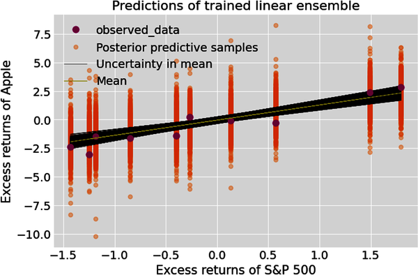
Predict and simulate test data
This creates a new inference group called predictions. We repeat the same steps as we did in the training phase but use test data instead:
# Get feature and target test data.feature_test=idata.predictions_constant_data['feature']target_test=idata.predictions_constant_data['target']# Prediction target values are in 2000 arrays, each with 10 samples,# the same number of samples as our test data set. Predict target values# based on posterior values of regression parameters and feature test data.prediction_target=posterior["alpha"]+posterior["beta"]*feature_test# Predictions is the data generating posterior predictive distribution# of the trained ensemble based on test data.simulate_predictions=idata.predictions['target_likelihood']# Create figure of subplots.fig,ax=plt.subplots()# Plot the 2000 regression lines showing the epistemic and# aleatory uncertainties of out-of-sample predictions.az.plot_lm(idata=idata,x=feature_test,y=target_test,num_samples=2000,y_model=prediction_target,y_hat=simulate_predictions,axes=ax)# Label figureax.set_xlabel("Excess returns of S&P 500")ax.set_ylabel("Excess returns of Apple")ax.set_title("Predictions of trained linear ensemble")ax.legend(loc='upper left');
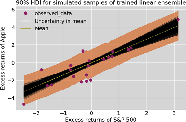
# Plot 90% HDI of trained ensemble. This will show the aleatory# (data related) and epistemic (parameter related) uncertainty# of trained model's predictions based on test data.# Create figure of subplots.fig,ax=plt.subplots()# Plot the ensemble of 2000 regression lines to show the epistemic uncertainty# around the mean regression line.az.plot_lm(idata=idata,x=feature_test,y=target_test,num_samples=2000,y_model=prediction_target,axes=ax)# Plot the posterior predictive data within the 90% HDI band# to show both epistemic and aleatory uncertainties.az.plot_hdi(feature_test,simulate_predictions,hdi_prob=0.90,smooth=False)# Label the figure.ax.set_xlabel("Excess returns of S&P 500")ax.set_ylabel("Excess returns of Apple")ax.set_title("90% HDI for predictions of trained linear ensemble")ax.legend();

Evaluate, revise, or deploy ensemble
From the recent plot we can see that our ensemble has simulated all of the test data within the 90% HDI band. Let’s also compute the probabilistic R-squared measure to evaluate the ensemble’s predictive performance:
# Evaluate out-of-sample predictions of trained# ensemble by comparing simulated data with test data.# Get target values of the test data.target_actual=target_test.values# Sample ensemble's predictions based on test data.target_predicted=idata.predictions.stack(sample=("chain","draw"))['target_likelihood'].values.T# Compute the probabilistic R-squared performance metric.test_score=az.r2_score(target_actual,target_predicted)test_score.round(2)
The probabilistic R-squared metric of the tested ensemble is 69%, with a standard deviation of 13%. It is better than our training score and exceeds the test score benchmark of 65%. We are ready to deploy our tested ensemble into our paper trading system or other simulated financial system that uses real-time data feeds with fictitious capital. This enables us to evaluate how our ensemble performs in real time before we are ready to deploy it into production and commit real hard-earned capital to our system.
Summary
In this chapter, we saw how probabilistic linear regression (PLE) modeling is fundamentally different from conventional linear regression (MLE) modeling. The probabilistic framework provides a systematic method for modeling physical phenomena in general and financial realities in particular.
Conventional financial models use the MLE method to compute the optimal values of parameters that fit the data. That would be appropriate if we were dealing with time-invariant statistical distributions. It is inappropriate in finance because we don’t have such time-invariant distributions. Learning optimal parameter values from noisy financial data is suboptimal and risky. Instead of relying on one expert in such a situation, we are better off relying on a council of experts for the many possible scenarios that are plausible and synthesize their expertise. This is exactly what a probabilistic ensemble does for us. It gives us the weighted average of all the estimates of model parameters.
In probabilistic regression modeling, as opposed to conventional linear modeling, data are treated as fixed and parameters are treated as variables because common sense and facts support such an approach. There is no need for the conventional use of ad hoc methods like L1 and L2 regularization, which are merely prior probability distributions in disguise. Most importantly, in the probabilistic paradigm, we are freed from ideological dictums like “let only the data speak for themselves” and unscientific claims of the existence of “true models” or “true parameters.”
Probabilistic ensembles make no pretense to analytical elegance. They do not lull us into a false sense of security about our financial activities with point estimates and bogus analytical solutions fit only for toy problems. Probabilistic ensembles are numerical and messy models that quantify aleatory and epistemic uncertainties. These models are suited for endemic uncertainties of finance and investing. Most importantly, it reminds us of the uncertainty of our knowledge, inferences, and predictions.
In the next chapter, we will explore how to apply our probabilistic estimates and predictions to decision making in the face of three-dimensional uncertainty and incomplete information.
References
Dürr, Oliver, and Beate Sick. Probabilistic Deep Learning with Python, Keras, and TensorFlow Probability. Manning Publications, 2020.
Gelman Andrew, Ben Goodrich, Jonah Gabry, and Aki Vehtari. “R-Squared for Bayesian Regression Models.” The American Statistician 73, no. 3 (2019): 307–309. https://doi.org/10.1080/00031305.2018.1549100.
Murphy, Kevin P. Machine Learning: A Probabilistic Perspective. Cambridge, MA: The MIT Press, 2012.
Further Reading
Martin, Osvaldo A., Ravin Kumar, and Junpeng Lao. Bayesian Modeling and Computation in Python. 1st ed. Boca Raton, FL: CRC Press, 2021.
1 Adapted from an image on Wikimedia Commons.
2 Oliver Dürr and Beate Sick, “Building Loss Functions with the Likelihood Approach,” in Probabilistic Deep Learning with Python, Keras, and TensorFlow Probability (Manning Publications, 2020), 93–127.
3 Kevin P. Murphy, “Sparse Linear Models,” in Machine Learning: A Probabilistic Perspective (Cambridge, MA: The MIT Press, 2012), 421–78.
4 Andrew Gelman et al., “R-Squared for Bayesian Regression Models,” The American Statistician 73, no. 3 (2019): 307–309, https://doi.org/10.1080/00031305.2018.1549100.