
CHAPTER 5
![]()
Looking Forward, a Standard for Performance
In Chapter 4 we built a JavaScript library to track ad hoc code and benchmark functions. This is a great tool to gather timing metrics and extrapolate performance gains through coding styles, as you’ll see in the coming chapters.
So far we’ve seen how to build our own tools, or use existing tools to gather the data that we need in order to measure performance, but now we will look at the work that the W3C has been doing to craft a standard for tracking performance metrics in browsers.
Note that some of these features are just now starting to be supported in modern browsers; some features are only available in beta and pre-beta versions of the browsers. For this reason I will identify the release version used in all of the examples in this chapter when relevant. It is also for this reason that I may show screen shots of the same thing but in different browsers, to illustrate the differing levels of support for these features.
W3C Web Performance Working Group
In late 2010 the W3C created a new working group, the Web Performance Working Group. The mission for this working group, as stated on its mission page, is to provide methods to measure aspects of application performance of user agent features and APIs. What that means in a very practical sense is that the working group has developed an API that browsers can and will expose to JavaScript that holds key performance metrics.
This is implemented in a new performance object that is part of the native window object:
>>window.performance
The Performance Object
If you type window.performance in a JavaScript console, you’ll see that it returns an object of type Performance with potentially several objects and methods that it exposes. Figure 5-1 shows the Performance object structure in Chrome 20 beta.
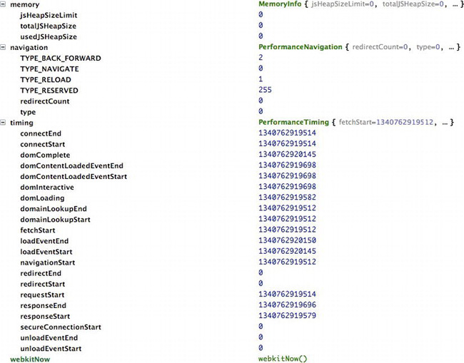
Figure 5-1. Window.performance in Chrome 20 beta
If we type this into Chrome we see that it supports a navigation object, of type PerformanceNavigation, and a timing object, of type PerformanceTiming. Chrome also supports a memory object, and webkitNow— a browser-specific version of High Resolution Time (I'll cover high-resolution time towards the end of this chapter).
Let’s take a look at each object and see how we can make use of these for our own performance tracking.
Performance Timing
The timing object has the following properties, all of which contain millisecond snapshots of when these events occur, much like our own startTimeLogging() function from last chapter. See Figure 5-2 for a flowchart of each timing metric in sequential order.
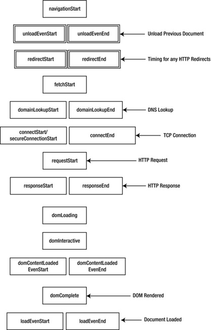
Figure 5-2. Sequential order of Performance metrics
navigationStart: This is the time snapshot for when navigation begins, either when the browser starts to unload the previous page if there is one, or if not, when it begins to fetch the content. It will either contain theunloadEventStartdata or thefetchStartdata. If we want to track end-to-end time we will often start with this value.
unloadEventStart: This is the time snapshot for when the browser begins to unload the previous page, if there is a previous page at the same domain to unload.
unloadEventEnd: This is the time snapshot for when the browser completes unloading the previous page.
redirectStart: This is the time snapshot for when the browser begins any HTTP redirects.
redirectEnd: This is the time snapshot for when all HTTP redirects are complete.
To calculate total time spent on HTTP redirects, simply subtract redirectStart from redirectEnd:
<script>

var http_redirect_time = performance.timing.redirectEnd - performance.timing.redirectStart;

</script>
fetchStart: This is the time snapshot for when the browser first begins to check the cache for the requested resource.
To calculate the total time spent loading cache, subtract fetchStart from domainLookupStart:
<script>

var cache_time = performance.timing.domainLookupStart - performance.timing.fetchStart;

</script>
domainLookupStart: This is the time snapshot for when the browser begins the DNS lookup for the requested content.
domainLookupEnd: This is the time snapshot for when the browser completes the DNS lookup for the requested content.
To calculate the total time spent on a DNS lookup, subtract the domainLookupStart from the domainLookupEnd:
<script>

var dns_time = performance.timing.domainLookupEnd - performance.timing.domainLookupStart;

</script>
connectStart: This is the time snapshot for when the browser begins establishing the TCP connection to the remote server for the current page.
secureConnectionStart:When the page is loaded over HTTPS, this property captures the time snapshot for when the HTTPS communication begins.
connectEnd: This is the time snapshot for when the browser finishes establishing the TCP connection to the remote server for the current page.
To calculate the total time spent establishing the TCP connection, subtract connectStart from connectEnd:
<script>

var tcp_connection_time = performance.timing.connectEnd - performance.timing.connectStart;

</script>
requestStart: This is the time snapshot for when the browser sends the HTTP request.
responseStart: This is the time snapshot for when the browser first registers the server response.
responseEnd: This is the time snapshot for when the browser finishes receiving the server response.
To calculate the total time spent on the complete HTTP roundtrip, including establishing the TCP connection, we can subtract connectStart from responseEnd:
<script>

var roundtrip_time = performance.timing.responseEnd - performance.timing.connectStart;

</script>
domLoading: This is the time snapshot for when the document begins loading.
domComplete: This is the time snapshot for when the document is finished loading.
To calculate the time spent rendering the page, we just subtract the domLoading from the domComplete:
<script>

var page_render_time = performance.timing.domComplete - performance.timing.domLoading;

</script>
To calculate the time spent loading the page, from the first request to when it is fully loaded, subtract navigationStart from domComplete:
<script>

var full_load_time =  performance.timing.domComplete - performance.timing.navigationStart

</script>
domContentLoadedEventEnd:This is fired when theDOMContentLoadedevent completes.
domContentLoadedEventStart:This is fired when theDOMContentLoadedevent begins.
The DOMContentLoaded event is fired when the browser completes parsing the document. For more information about this event, see the W3C’s documentation for the steps that happen at the end of the document parsing, located at http://www.w3.org/TR/html5/the-end.html.
domInteractive:This is fired when the document’sreadyStateproperty is set to interactive, indicating that the user can now interact with the page.
loadEventEnd:This is fired when the load event of the document is finished.
loadEventStart:This is fired when the load even of the document starts.
Let’s update perfLogger to use this new-found wealth of performance data! We’ll add read-only public properties that will return calculated values that we want to record. We’ll also update the prototype of the Test Result object so that each result we send to the server automatically has these performance metrics built in.
Let’s get started!
Integrating the Performance Object with perfLogger
First, you need to create private variables in the self-executing function of perfLogger. Create values for perceived time, redirect time, cache time, DNS lookup time, TCP connection time, total round trip time, and page render time:
var perfLogger = function(){ var serverLogURL = "savePerfData.php",
loggerPool = [];
if(window.performance){
var _pTime = Date.now() - performance.timing.navigationStart || 0,
_redirTime = performance.timing.redirectEnd - performance.timing.redirectStart || 0,
_cacheTime = performance.timing.domainLookupStart - performance.timing.fetchStart || 0,
_dnsTime = performance.timing.domainLookupEnd - performance.timing.domainLookupStart || 0,
_tcpTime = performance.timing.connectEnd - performance.timing.connectStart || 0,
_roundtripTime = performance.timing.responseEnd - performance.timing.connectStart || 0,
_renderTime = performance.timing.domComplete - performance.timing.domLoading || 0;
}
}
First this code wraps our variable assignments in an if statement to make sure we only invoke window.performance if the current browser supports it. Then note that we are using short circuit evaluation when assigning these variables. This technique uses a logic operator—in this case a logical OR—in the variable assignments. If the first value is unavailable, null or undefined, then the second value is used in the assignment.
Next, still within the self-executing function, you’ll explicitly create a TestResults constructor. Remember that we architected the TestResults object last chapter, but we never ended up using it, instead we had loggerPool hold general objects. You’re going to use TestResults now, and take advantage of prototypal inheritance to make sure each TestResults object has our new performance metrics built in.
First create the TestResults constructor.
function TestResults(){};
Then add a property to the prototype of TestResults for each of our window.performance metrics:
TestResults.prototype.perceivedTime = _pTime;

TestResults.prototype.redirectTime = _redirTime;

TestResults.prototype.cacheTime = _cacheTime;

TestResults.prototype.dnsLookupTime = _dnsTime;

TestResults.prototype.tcpConnectionTime = _tcpTime;

TestResults.prototype.roundTripTime = _roundtripTime;

TestResults.prototype.pageRenderTime = _renderTime;
Excellent! Now let’s go and edit our public method startTimeLogging(). Right now the first line of the function assigns an empty object to loggerPool:
loggerPool[id] = {};
Change that to instead instantiate a new instance of TestResults:
At this point if you console.log a TestResults object, it should look like Figure 5-3.
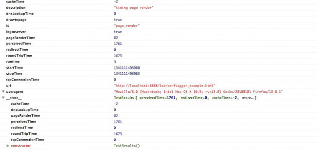
Figure 5-3. TestResults object
You can see that we now have cacheTime, dnsLookupTime, pageRenderTime, perceivedTime, redirectTime, roundTripTime, and tcpConnectionTime properties for each TestResults object that we create. You can also see that these properties exist on the prototype.
This is an important point, because if you console.log the serialized object in logToServer() you will see that those properties are not serialized with the rest of the object. This is because JSON.stringify does not serialize undefined values or functions within an object.
That’s not a problem, though. To solve this, you just need to make a small private function to concatenate two objects. Sogo back to the self-executing function at the top, where you’ll add a new function jsonConcat() and have it accept two objects:
function jsonConcat(object1, object2) {}
Next loop through each property in the second object and add the properties to the first object. Finally, return the first object:
for (var key in object2) {

object1[key] = object2[key];

}

return object1;
Note that this will also overwrite the values of any properties in the first object that the two objects may have in common.
The finished function should look like this.
function jsonConcat(object1, object2) {

for (var key in object2) {

object1[key] = object2[key];

     }
     return object1;

}
Now to make this work, go back to logToServer(). Recall that in the beginning of the function we serialize our TestResults object this way:
var params = "data=" + (JSON.stringify(loggerPool[id]));
Change that to pass the TestResults object and its prototype into jsonConcat(), and pass the returned object to JSON.stringify:
var params = "data=" + JSON.stringify(jsonConcat(loggerPool[id],TestResults.prototype));
If you console.log the params variable, it should look like this:
data={"id":"page_render","startTime":1341152573075,"description":"timing page render","drawtopag

e":true,"logtoserver":true,"stopTime":1341152573077,"runtime":2,"url":"http://localhost:8888/

lab/perfLogger_example.html","useragent":"Mozilla/5.0 (Macintosh; Intel Mac OS X 10.5; rv:13.0)

Gecko/20100101 Firefox/13.0.1","perceivedTime":78,"redirectTime":0,"cacheTime":-2,"dnsLookupTime

":0,"tcpConnectionTime":0,"roundTripTime":2,"pageRenderTime":72}
Next you’ll expose these private performance variables via public methods in order to expose them via the perfLogger namespace without needing to run any tests. If you didn’t expose the variables at the object level, you would need to create a test and pull them from the test object; recall that we added these Performance object numbers to the prototype of every test object.
//expose derived performance data

perceivedTime: function(){

return _pTime;

},

redirectTime: function(){

     _redirTime;

},

cacheTime: function(){

     return _cacheTime;

},

dnsLookupTime: function(){

     return _dnsTime;

},

tcpConnectionTime: function(){

     return _tcpTime;

},

roundTripTime: function(){

     return _roundtripTime;

},

pageRenderTime: function(){

     return _renderTime;

}
Excellent! These public functions expose the data from the perfLogger object like so:
>>> perfLogger.perceivedTime()

78
So now your updated perfLogger.js should look like this:
var perfLogger = function(){

var serverLogURL = "savePerfData.php",

     loggerPool = [],

     _pTime = Date.now() - performance.timing.navigationStart || 0,

     _redirTime = performance.timing.redirectEnd - performance.timing.redirectStart || 0,

     _cacheTime = performance.timing.domainLookupStart - performance.timing.fetchStart || 0,

     _dnsTime = performance.timing.domainLookupEnd - performance.timing.domainLookupStart || 0,

     _tcpTime = performance.timing.connectEnd - performance.timing.connectStart || 0,

     _roundtripTime = performance.timing.responseEnd - performance.timing.connectStart || 0,

     _renderTime = Date.now() - performance.timing.domLoading || 0;


function TestResults(){};

TestResults.prototype.perceivedTime = _pTime;

TestResults.prototype.redirectTime = _redirTime;

TestResults.prototype.cacheTime = _cacheTime;

TestResults.prototype.dnsLookupTime = _dnsTime;

TestResults.prototype.tcpConnectionTime = _tcpTime;

TestResults.prototype.roundTripTime = _roundtripTime;

TestResults.prototype.pageRenderTime = _renderTime;


function jsonConcat(object1, object2) {

for (var key in object2) {

     object1[key] = object2[key];

}

return object1;

}


function calculateResults(id){

     loggerPool[id].runtime = loggerPool[id].stopTime - loggerPool[id].startTime;

}


function setResultsMetaData(id){

     loggerPool[id].url = window.location.href;

     loggerPool[id].useragent = navigator.userAgent;

}


function drawToDebugScreen(id){

     var debug = document.getElementById("debug")

     var output = formatDebugInfo(id)

     if(!debug){

          var divTag = document.createElement("div");

          divTag.id = "debug";

          divTag.innerHTML = output

          document.body.appendChild(divTag);

     }else{

          debug.innerHTML += output

     }

}


function logToServer(id){

     var params = "data=" + JSON.stringify(jsonConcat(loggerPool[id],TestResults.prototype));
     var xhr = new XMLHttpRequest();

     xhr.open("POST", serverLogURL, true);

     xhr.setRequestHeader("Content-type", "application/x-www-form-urlencoded");

     xhr.setRequestHeader("Content-length", params.length);

     xhr.setRequestHeader("Connection", "close");

     xhr.onreadystatechange = function()

      {

      if (xhr.readyState==4 && xhr.status==200)

        {}

      };

     xhr.send(params);

}


function formatDebugInfo(id){

     var debuginfo = "<p><strong>" + loggerPool[id].description + "</strong><br/>";

     if(loggerPool[id].avgRunTime){

          debuginfo += "average run time: " + loggerPool[id].avgRunTime + "ms<br/>";

     }else{

          debuginfo += "run time: " + loggerPool[id].runtime + "ms<br/>";

     }

     debuginfo += "path: " + loggerPool[id].url + "<br/>";

     debuginfo += "useragent: " +  loggerPool[id].useragent + "<br/>";

     debuginfo += "</p>";

     return debuginfo

}


return {


startTimeLogging: function(id, descr,drawToPage,logToServer){

loggerPool[id] = new TestResults();

     loggerPool[id].id = id;

     loggerPool[id].startTime =  Date.now();

     loggerPool[id].description = descr;

     loggerPool[id].drawtopage = drawToPage;

     loggerPool[id].logtoserver = logToServer

},


stopTimeLogging: function(id){

loggerPool[id].stopTime =  Date.now();

     calculateResults(id);

     setResultsMetaData(id);

     if(loggerPool[id].drawtopage){

          drawToDebugScreen(id);

     }

     if(loggerPool[id].logtoserver){

          logToServer(id);

     }

},


logBenchmark: function(id, timestoIterate, func, debug, log){

     var timeSum = 0;
     for(var x = 0; x < timestoIterate; x++){

          perfLogger.startTimeLogging(id, "benchmarking "+ func, false, false);

          func();

          perfLogger.stopTimeLogging(id)

          timeSum += loggerPool[id].runtime

     }

     loggerPool[id].avgRunTime = timeSum/timestoIterate

     if(debug){

          drawToDebugScreen(id)

     }

     if(log){

          logToServer(id)

     }

},


//expose derived performance data

perceivedTime: function(){

return _pTime;

},

redirectTime: function(){

     _redirTime;

},

cacheTime: function(){

     return _cacheTime;

},

dnsLookupTime: function(){

     return _dnsTime;

},

tcpConnectionTime: function(){

     return _tcpTime;

},

roundTripTime: function(){

     return _roundtripTime;

},

pageRenderTime: function(){

     return _renderTime;

}

}

}();
Updating the Logging Functionality
Let’s next update our savePerfData.php file. Start by adding new headers to the formatNewLog() function, so that each new log file to be created has column headers for our new data points:
function formatNewLog($file){

     $headerline = "IP, TestID, StartTime, StopTime, RunTime, URL, UserAgent, PerceivedLoadTime,

PageRenderTime, RoundTripTime, TCPConnectionTime, DNSLookupTime, CacheTime, RedirectTime";

     appendToFile($headerline, $file);

}
Then update saveLog() to include the additional values that we are now passing in:
function saveLog($obj, $file){

     if(!file_exists($file)){

          formatNewLog($file);

     }

     $obj->useragent = cleanCommas($obj->useragent);

     $newLine = $_SERVER["REMOTE_ADDR"] . "," . $obj->id .",". $obj->startTime . "," . $obj-

>stopTime . "," . $obj->runtime . "," . $obj->url . "," . $obj->useragent . "," . $obj-

>perceivedTime . "," . $obj->pageRenderTime . "," . $obj->roundTripTime . "," . $obj-

>tcpConnectionTime . "," . $obj->dnsLookupTime . "," . $obj->cacheTime . "," . $obj-

>redirectTime;

     appendToFile($newLine, $file);

}
The updated log file should now look like this:
IP, TestID, StartTime, StopTime, RunTime, URL, UserAgent, PerceivedLoadTime, PageRenderTime,

RoundTripTime, TCPConnectionTime, DNSLookupTime, CacheTime, RedirectTime

127.0.0.1,page_render,1.34116648339,1.3411664834,2,http://localhost:8888/lab/perfLogger_example.

html,Mozilla/5.0 (Macintosh; Intel Mac OS X 10.5; rv:13.0) Gecko/20100101 Firef

ox/13.0.1115,86,21,1,1,-4,0

127.0.0.1,page_render,345.173000009,345.331000019,0.158000009833,http://localhost:8888/lab/

perfLogger_example.html,Mozilla/5.0 (Macintosh; Intel Mac OS X 10_5_8) AppleWebKit/536.11 (KHTML

like Gecko) Chrome/20.0.1132.43 Safari/536.11495,261,79,0,0,0,0
Performance Navigation
Let's now take a look at the Performance Navigation object. If you type performance.navigation into your console, you’ll see something like Figure 5-4.

Figure 5-4. Performance Navigation object
Note that the navigation object has two read-only attributes: redirectCount and type. The redirectCount attribute is exactly what it sounds like, the number of HTTP redirects that the browser follows to get to the current page.
![]() Note: HTTP redirects are significant because they cause a complete roundtrip for each redirect. The original request is returned from the web server as either a 301 or a 302 with the path to the new location. The browser must then initialize a new TCP connection and send a new request for the new location. See Figure 5-5 for a sequence diagram of a single HTTP redirect. Note how the DNS lookup, the TCP handshake, and the HTTP request are all repeated for the redirected asset. This repetition doubles the network connection time for a single redirect.
Note: HTTP redirects are significant because they cause a complete roundtrip for each redirect. The original request is returned from the web server as either a 301 or a 302 with the path to the new location. The browser must then initialize a new TCP connection and send a new request for the new location. See Figure 5-5 for a sequence diagram of a single HTTP redirect. Note how the DNS lookup, the TCP handshake, and the HTTP request are all repeated for the redirected asset. This repetition doubles the network connection time for a single redirect.

Figure 5-5. HTTP Redirect
We can access the redirectCount property like so:
>>> performance.navigation.redirectCount

0
The other attribute of the navigation object is type. The navigation.type attribute will be one of four values represented by the following constants:
TYPE_NAVIGATE:Has the value of 0, which indicates that the current page was navigated to by clicking on a link, submitting a form, or entering the URL directly in the address bar.
TYPE_RELOAD:Has the value of 1, indicating that the current page was arrived at via a reload operation.
TYPE_BACK_FORWARD:Has the value of 2, indicating that the page was navigated to via the browser history, either using the back or forward buttons or programmatically through the browser’s history object.
TYPE_RESERVED:Has the value of 255 and is a catch-all for any navigation type not defined above.
Performance Memory
The memory object is a feature of Chrome that allows us to see the memory usage that Chrome is taking up while running our page. Notice in Figure 5-1 earlier that all of the values return 0—that is because we need to enable the memory info flag before we can take advantage of this capability.
The way to do this is slightly platform dependent, but essentially you need to pass the --enable-memory-info command-line parameter into Chrome. To do this on a Windows platform, right-click the Chrome icon, go to Properties, and at the end of the path to the executable, append the flag --enable-memory-info. The executable should look like this:
[path to exe]chrome.exe --enable-memory-info
For the Mac OS, instead of updating a shortcut, go into Terminal and invoke the Chrome application like so:
/Applications/Google Chrome.app/Contents/MacOS/Google Chrome --enable-memory-info
For more information, see http://www.chromium.org/developers/how-tos/run-chromium-with-flags.
Once you launch Chrome with the flag enabled, you should see data now in the memory object, as in Figure 5-6.
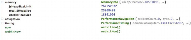
Figure 5-6. Performance Memory object with data
For reference, the heap is the collection of JavaScript objects that the interpreter keeps in resident memory. In the heap each object is an interconnected node, connected via properties, like the prototype chain, or composed objects. JavaScript running in the browser references the objects in the heap via object references, as diagrammed in Figure 5-7. When we destroy an object in JavaScript, what we are really doing is destroying the object reference. When the interpreter sees an object in the heap with no object references, it removes that object from the heap. This is called garbage collection.

Figure 5-7. the JavaScript Heap
The usedJsHeapSize property shown in Figure 5-6 is the amount of memory that all of the current objects in the heap are using. The totalJsHeapSize is size of the heap including free space not used by objects.
Because we need to launch the browser with command-line parameters to get these properties, this isn’t something that we can include in our library and put out in our production environment and hope to get real data from it. Instead it is a tool we can monitor and run in our own lab for profiling purposes.
![]() Note: Profiling allows us to monitor our memory usage. This is useful for detecting memory leaks, the creation of objects that never get destroyed. Usually in JavaScript this occurs when we programmatically assign event handlers to DOM objects and forget to remove the event handlers. More nuanced than just detecting leakages, profiling is also useful for optimizing the memory usage of our applications over time. We should intelligently create, destroy, or re-use objects and always be mindful of scope to avoid profiling charts that trend upward in an ever-growing series of spikes. A much better profile chart shows a controlled rise and plateau.
Note: Profiling allows us to monitor our memory usage. This is useful for detecting memory leaks, the creation of objects that never get destroyed. Usually in JavaScript this occurs when we programmatically assign event handlers to DOM objects and forget to remove the event handlers. More nuanced than just detecting leakages, profiling is also useful for optimizing the memory usage of our applications over time. We should intelligently create, destroy, or re-use objects and always be mindful of scope to avoid profiling charts that trend upward in an ever-growing series of spikes. A much better profile chart shows a controlled rise and plateau.
Firefox has started allowing insight into its memory usage as well. Typing about:memory into the location bar brings up a page that gives a high-level breakdown of memory usage; to get a more granular insight, type about:memory?verbose. See Figure 5-8 for the resulting granular breakdown of memory usage in Firefox.

Figure 5-8. Firefox memory window
High-Resolution Time
The next change we will look at is a feature called high-resolution time— time recorded in sub-millisecond values. This is useful for capturing timing data that happens in less than 1 millisecond. We’ll make extensive use of high-resolution time in the next chapter to capture run time performance metrics.
The Web Performance Working Group has detailed a public method of the performance object, performance.now().
As you saw in the previous chapter, when timing code execution we ran into cases where we had 0 millisecond results. That is because the values that are returned from the Date() object only had precision to up to 1 millisecond. Type the following into a JavaScript console to see the Date() object:
>>> new Date().getMilliseconds()

603

>>> Date.now()

1340722684122
Because of refinements in the performance of JavaScript interpreters and browser rendering engines, some of our operations may complete within microseconds. That’s when we get 0 millisecond results for our tests.
A more subtle danger with this sort of test is that the value in the Date object is based on system date, which theoretically can be changed during a test, and would skew the results. Any number of things could change the system date without our input, from daylight savings time adherence, to corporate policy synchronizing system times. And any of these would change our timed results, even to potentially negative results.
The performance.now() method returns results in fractions of milliseconds. It also is relative to the navigationStart event, not the system date, so it will not be impacted by changing system time. Chrome started supporting high-resolution time with Chrome 20 via the browser-specific prefixed webkitNow() function, which looks like this:
Google Chrome 20

>>> performance.webkitNow()

290117.4699999974
And Firefox began supporting high-resolution time with Firefox 15 Aurora release:
Firefox 15 aurora

>>> performance.now()

56491.447434
This is great, but how do we start to use this now, and how do we make sure the code that we write now will be relevant once this is supported in all browsers? To future-proof our perfLogger library, we can code against the performance.now() method and build in a shim for a fallback if the browser does not yet support it.
![]() Note: A shim is an abstraction layer that intercepts API calls or events and either changes the signature of the call and passes on the call to fit an updated API signature, or handles the functionality of the API itself. Figure 5-9 diagrams a shim intercepting an event or message dispatch, presumably to perform some logic, before republishing out the message. Figure 5-10 diagrams a shim that is overriding a function or an object, processes the information, and then either passes data to, or invokes via composition, the original object or function.
Note: A shim is an abstraction layer that intercepts API calls or events and either changes the signature of the call and passes on the call to fit an updated API signature, or handles the functionality of the API itself. Figure 5-9 diagrams a shim intercepting an event or message dispatch, presumably to perform some logic, before republishing out the message. Figure 5-10 diagrams a shim that is overriding a function or an object, processes the information, and then either passes data to, or invokes via composition, the original object or function.

Figure 5-9. Intercept

In this case you will override the performance.now() function call and add a layer of functionality before passing it on or handling it ourselves.
In perfLogger.js, after the perfLogger self-executing function, add a function declaration to override the native call to performance.now:
performance.now = (function() {

})();
This function should return performance.now if it is supported; if it is not, the code iterates through the potential browser-specific implementations, and if none of those are supported it defaults to the old Date() functionality.
performance.now = (function() {

return performance.now       ||

          performance.webkitNow ||

          function() { return new Date().getTime(); };

})();
Next update perfLogger’s startTimeLogging() and stopTimeLogging() functions to use performance.now():
startTimeLogging: function(id, descr,drawToPage,logToServer){

loggerPool[id] = {};

     loggerPool[id].id = id;

     loggerPool[id].startTime =  performance.now(); // high resolution time support

     loggerPool[id].description = descr;

     loggerPool[id].drawtopage = drawToPage;

     loggerPool[id].logtoserver = logToServer

}


stopTimeLogging: function(id){

loggerPool[id].stopTime =  performance.now(); //high resolution time support

     calculateResults(id);

     setResultsMetaData(id);

     if(loggerPool[id].drawtopage){

          drawToDebugScreen(id);

     }

     if(loggerPool[id].logtoserver){

          logToServer(id);

     }
}
Now let’s take a look at what the page render benchmarking results from last chapter look like with browsers that support high-resolution time. In Figure 5-11, we’ll look at our results in Chrome 19 to see how the browser reacts without the support of high-resolution time. In Figure 5-12, we’ll see our results in Firefox 15 Aurora release; and in Figure 5-13, we’ll see our results in Chrome 20, as both browsers support high-resolution time.

Figure 5-11. Chrome 19 defaulting to Date object

Figure 5-12. Firefox 15 Aurora release supports performance.now

Figure 5-13. Chrome 20 supports performance.webkitNow
At this point you’ve integrated the new Performance object into the perfLogger library and added several new columns to our log file. These new data points add additional dimensions for analyzing our data. With our new capability of capturing high-resolution time we are set up perfectly to begin gathering runtime metrics next chapter.
Visualizing the New Data
Now let’s have some fun with our new data! There are some great data points that we can look at: What is our average load time user agent? On average, what part of the HTTP transaction process takes the most time? And what is our general load time distribution? So let’s get started.
A sample of our data looks like this:
IP, TestID, StartTime, StopTime, RunTime, URL, UserAgent, PerceivedLoadTime, PageRenderTime,

RoundTripTime, TCPConnectionTime, DNSLookupTime, CacheTime, RedirectTime

75.149.106.130,page_render,1341243219599,1341243220218,619,http://www.tom-barker.com/

blog/?p=x,Mozilla/5.0 (Macintosh; Intel Mac OS X 10.5; rv:13.0) Gecko/20100101 Firef

ox/13.0.1790,261,-2,36,0,-4,0

75.149.106.130,page_render,633.36499998695,973.8049999869,340.43999999994,http://www.tom-barker.

com/blog/?p=x,Mozilla/5.0 (Macintosh; Intel Mac OS X 10_5_8) AppleWebKit/536.11 (KHTML like

Gecko) Chrome/20.0.1132.43 Safari/536.11633,156,-1341243238576,30,0,0,0

75.149.106.130,page_render,1498.2289999898,2287.9749999847,789.74599999492,http://www.tom-

barker.com/blog/?p=x,Mozilla/5.0 (Macintosh; Intel Mac OS X 10_5_8) AppleWebKit/536.11 (KHTML

like Gecko) Chrome/20.0.1132.43 Safari/536.111497,979,788,0,0,0,0
First let’s look at the frequency distribution of perceived load times. at a large enough scale, this will give us a pretty good idea of what the general experience is like for most users. We already have performance data being read into the perflogs variable back from the R script that we’ve been assembling since Chapter 3, so let’s just draw a histogram using that variable:
hist(perflogs$PerceivedLoadTime, main="Distribution of Perceived Load

Time", xlab="Perceived Load Time in Milliseconds", col=c("#CCCCCC"))
This creates the graph that we see in Figure 5-14.
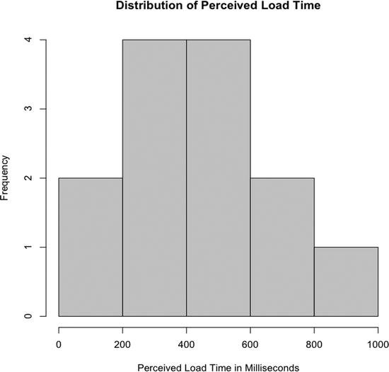
Figure 5-14. Histogram of perceived load time, frequency representing number of visits
Pretty simple so far. You just need to wrap it in a call to the pdf() function to save this as a file we can reference later:
loadTimeDistrchart <- paste(chartDirectory, "loadtime_distribution.pdf", sep="")

pdf(loadTimeDistrchart, width=10, height=10)

     hist(perflogs$Perceived

LoadTime, main="Distribution of Perceived Load Time", xlab="Perceived Load Time in Milliseconds", col=c("#CCCCCC"))

dev.off()
Now let’s take a look at all of the data that we have collected from our full HTTP request and break down the average time spent on each part of the request. This will give us a full picture of how long each step takes.
First create a new variable to hold the path to our next chart, and a new function to hold this in, called avgTimeBreakdownInRequest:
requestBreakdown <- paste(chartDirectory, "avgtime_inrequest.pdf", sep="")

avgTimeBreakdownInRequest <- function(){

}
Within the function you’ll do some things to clean up the data. If the numbers are large enough, R may store them in exponential notation. This is great for referencing large numbers, but to visualize these numbers for general consumption we should unfurl the exponential notation for ease of reading. To do this, pass the scipen parameter to the options() function. The options() function allows us to set global options in R, and scipen takes a numeric value; the higher the value passed in, the greater the chance that R will display numbers in fixed position, not in exponential notation:
options(scipen=100)
Next address some of those negative numbers that we see in the data. Negative numbers don’t make sense in this context. They appear because sometimes the window.performance object returns 0 for values, and we are doing subtraction between values to derive our saved performance data.
You have some choices here; you could remove the rows where negative numbers occur, or just zero out the negatives. You could wipe out the whole row if you thought one bad column indicated that the rest of the row was unreliable, but that’s not the case here. To avoid losing the values in the other columns that may be good, just zero out the negatives.
To zero out the negatives, we simply check for any values that are less than 0 in each column, and set those columns to 0. Do this for each column to graph:
perflogs$PageRenderTime[perflogs$PageRenderTime < 0] <- 0

perflogs$RoundTripTime[perflogs$RoundTripTime < 0] <- 0

perflogs$

TCPConnectionTime[perflogs$TCPConnectionTime < 0] <- 0

perflogs$DNSLookupTime[perflogs$DNSLookupTime < 0] <- 0
Next you will create a data frame that contains the average value for each column. To do this, use the data.frame() function and pass in a call to mean() for each column that should be averaged. Then set the column names for this new data frame:
avgTimes <- data.frame(mean(perflogs$PageRenderTime), mean(perflogs$RoundTripTime), mean(perflogs$T

CPConnectionTime), mean(perflogs$DNSLookupTime))


colnames(avgTimes) <- c("PageRenderTime", "RoundTripTime", "TCPConnectionTime", "DNSLookupTime")
Finally, create the chart. It will be a horizontal bar chart, much like we’ve made in previous chapters, and save this as a PDF.
pdf(requestBreakdown, width=10, height=10)

opar <- par(no.readonly=TRUE)

     par(las=1, mar=c(10,10,10,10))

     barplot(as.matrix(avgTimes), horiz=TRUE, main="Average Time Spent
During HTTP Request",

xlab="Milliseconds")

par(opar)

dev.off()
Your completed function should look as follows, and the chart it generates can be seen in Figure 5-15.
avgTimeBreakdownInRequest <- function(){

#expand exponential notation

options(scipen=100)


#set any negative values to 0
perflogs$PageRenderTime[perflogs$PageRenderTime < 0] <- 0

perflogs$RoundTripTime[perflogs$RoundTripTime < 0] <- 0

perflogs$TCPConnectionTime[perflogs$TCPConnectionTime < 0] <- 0

perflogs$DNSLookupTime[perflogs$DNSLookupTime < 0] <- 0


#capture avg times

avgTimes <- data.frame(mean(perflogs$PageRenderTime), mean(perflogs$RoundTripTime), mean(perflogs$TCPConnectionTime), mean(perflogs$DNSLookupTime))

colnames(avgTimes) <- c("PageRenderTime", "RoundTripTime", "TCPConnectionTime", "DNSLookupTime")


pdf(requestBreakdown, width=10, height=10)

opar <- par(no.readonly=TRUE)

     par(las=1, mar=c(10,10,10,10))

     barplot(as.matrix(avgTimes), horiz=TRUE, main="Average Time Spent
During HTTP Request",

xlab="Milliseconds")

par(opar)

dev.off()

}
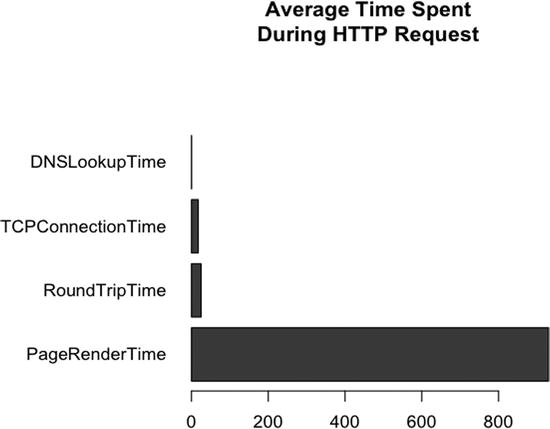
Figure 5-15. Avg Time for each step in HTTP Request
This is an interesting result. You may have figured already that the rendering of the page would take the longest, since it would have the most overhead and the most to do; it’s making sense of the message, not just transmitting it. But you may not have thought that the TCP connection time and round trip time were the same or that they would be so significantly higher than the DNS lookup time.
The final chart that we’ll look at for this chapter is a breakdown of perceived load time by browser. Notice that the sample data above stores the full user agent string, which gives not just the browser name, but the version, the sub-version, the operating system, and even the render engine. This is great, but if you want to roll up to a high level of browser information, irrespective of versioning or OS, we can search the user agent string for the specific high level browser name.
You can search for strings in data frame columns using grep(). The grep() function accepts the string to search for as its first parameter and the vector or object to search through as the second parameter. For our purposes we’ll use the grep() function as a filtering option that we pass into a data frame:
data frame[grep([string to search for], [data frame column to search])]
Create a function called getDFByBrowser() that will allow you to generalize the search by passing in a data frame to search and a string to search for:
getDFByBrowser<-function(data, browsername){

     return(data[grep(browsername, data$UserAgent),])

}
Next create a variable to hold the path to our new chart, loadtime_bybrowser:
loadtime_bybrowser <- paste(chartDirectory, "loadtime_bybrowser.pdf", sep="")
Next create a function to hold the main functionality for this chart; call it printLoadTimebyBrowser():
printLoadTimebyBrowser <- function(){

}
This function first creates data frames for each browser that we want to include in our graph:
chrome <- getDFByBrowser(perflogs, "Chrome")

firefox <- getDFByBrowser(perflogs, "Firefox")

ie <- getDFByBrowser(perflogs, "MSIE")
Next create a data frame to hold the average perceived load time for each browser, much as you did in the previous example for steps in the HTTP request. Also give the data frame descriptive column names:
meanTimes <- data.frame(mean(chrome$PerceivedLoadTime), mean(firefox$PerceivedLoadTime),

mean(ie$PerceivedLoadTime))

colnames(meanTimes) <- c("Chrome", "Firefox", "Internet Explorer")
And finally, create the graph as a bar chart and save it as a pdf:
pdf(loadtime_bybrowser, width=10, height=10)

     barplot(as.matrix(meanTimes), main="Average Perceived Load Time
By Browser", ylim=c(0,

600), ylab="milliseconds")

dev.off()
Your completed functionality should look like the following, and the finished chart should look like Figure 5-16.
getDFByBrowser<-function(data, browsername){

     return(data[grep(browsername, data$UserAgent),])

}


printLoadTimebyBrowser <- function(){

     chrome <- getDFByBrowser(perflogs, "Chrome")

     firefox <- getDFByBrowser(perflogs, "Firefox")

     ie <- getDFByBrowser(perflogs, "MSIE")

     meanTimes <- data.frame(mean(chrome$PerceivedLoadTime), mean(firefox$PerceivedLoadTime),

mean(ie$PerceivedLoadTime))

     colnames(meanTimes) <- c("Chrome", "Firefox", "Internet Explorer")
     pdf(loadtime_bybrowser, width=10, height=10)

          barplot(as.matrix(meanTimes), main="Average Perceived Load Time
By Browser",

ylim=c(0, 600), ylab="milliseconds")

     dev.off()

}
Figure 5-16 Average perceived load time by browser
Interestingly enough, the results of our tests show that Firefox has the best perceived load time, followed by Chrome, and finally Internet Explorer. This is just the smallest taste of a comparison; we could expand this by looking at versions and sub-versions if we wanted to.
The full updated R file should now look like this:
dataDirectory <- "/Applications/MAMP/htdocs/lab/log/"

chartDirectory <- "/Applications/MAMP/htdocs/lab/charts/"

testname = "page_render"


perflogs <- read.table(paste(dataDirectory, "runtimeperf_results.csv", sep=""), header=TRUE,

sep=",")

perfchart <- paste(chartDirectory, "runtime_",testname, ".pdf", sep="")


loadTimeDistrchart <- paste(chartDirectory, "loadtime_distribution.pdf", sep="")

requestBreakdown <- paste(chartDirectory, "avgtime_inrequest.pdf", sep="")

loadtime_bybrowser <- paste(chartDirectory, "loadtime_bybrowser.pdf", sep="")
pagerender <- perflogs[perflogs$TestID == "page_render",]

df <- data.frame(pagerender$UserAgent, pagerender$RunTime)

df <- by(df$pagerender.RunTime, df$pagerender.UserAgent, mean)

df <- df[order(df)]


pdf(perfchart, width=10, height=10)

opar <- par(no.readonly=TRUE)

     par(las=1, mar=c(10,10,10,10))

     barplot(df, horiz=TRUE)

par(opar)

dev.off()


getDFByBrowser<-function(data, browsername){

     return(data[grep(browsername, data$UserAgent),])

}


printLoadTimebyBrowser <- function(){

     chrome <- getDFByBrowser(perflogs, "Chrome")

     firefox <- getDFByBrowser(perflogs, "Firefox")

     ie <- getDFByBrowser(perflogs, "MSIE")


     meanTimes <- data.frame(mean(chrome$PerceivedLoadTime), mean(firefox$PerceivedLoadTime),

mean(ie$PerceivedLoadTime))

     colnames(meanTimes) <- c("Chrome", "Firefox", "Internet Explorer")

     pdf(loadtime_bybrowser, width=10, height=10)

          barplot(as.matrix(meanTimes), main="Average Perceived Load Time
By Browser",

ylim=c(0, 600), ylab="milliseconds")

     dev.off()

}


pdf(loadTimeDistrchart, width=10, height=10)

     hist(perflogs$PerceivedLoadTime, main="Distribution of Perceived Load Time", xlab="Perceived

Load Time in Milliseconds", col=c("#CCCCCC"))

dev.off()


avgTimeBreakdownInRequest <- function(){


#expand exponential notation

options(scipen=100, digits=3)


#set any negative values to 0

perflogs$PageRenderTime[perflogs$PageRenderTime < 0] <- 0

perflogs$RoundTripTime[perflogs$RoundTripTime < 0] <- 0

perflogs$TCPConnectionTime[perflogs$TCPConnectionTime < 0] <- 0

perflogs$DNSLookupTime[perflogs$DNSLookupTime < 0] <- 0


#capture avg times
avgTimes <- data.frame(mean(perflogs$PageRenderTime), mean(perflogs$RoundTripTime), mean(perflogs$T

CPConnectionTime), mean(perflogs$DNSLookupTime))

colnames(avgTimes) <- c("PageRenderTime", "RoundTripTime", "TCPConnectionTime", "DNSLookupTime")

pdf(requestBreakdown, width=10, height=10)

opar <- par(no.readonly=TRUE)

     par(las=1, mar=c(10,10,10,10))

     barplot(as.matrix(avgTimes), horiz=TRUE, main="Average Time Spent
During HTTP Request",

xlab="Milliseconds")

par(opar)

dev.off()


}


#invoke our new functions

printLoadTimebyBrowser()

avgTimeBreakdownInRequest()
Summary
This chapter explored the window.performance object, a new standardized way from the W3C to gather performance metrics from the browser. We incorporated the Performance object into our existing perfLogger project, including the performance metrics in each test that we run, as well as building in support for window.performance’s high-resolution time, if the browser supports it.
We used this new data to look at the overall web performance of our sites.
We touched upon the emerging possibilities of looking at client machine memory usage from a browser, specifically Chrome’s implementation, and a brief look at how to get Firefox to expose similar data.
The next chapter will take a look at optimizing web performance; you will run multivariate tests with the tools that we’ve developed to look at the results of our optimizations.