CHAPTER 2

Tools and Technology to Measure and Impact Performance

Chapter 1 outlined the concepts of web performance and runtime performance and discussed influencing factors for each. This chapter will look at some of the tools that are available to track performance and to help improve performance.

In future chapters we will explore how to use some of these tools programmatically and combine them to create charting and reporting applications, so getting familiar with them first is essential. Other tools, like Firebug and YSlow, are just essential tools for developing and maintaining performant web sites.

Firebug

2006 was a great year for web development. First of all, Microsoft released Internet Explorer 7, which brought with it native JavaScript support for the XMLHttpRequest object—previously web developers had to branch their code. If a browser’s JavaScript engine supported XHR we would use that; otherwise we would know that we were in an earlier version of IE and instantiate the XHR ActiveX control.

A slew of new frameworks also came out in 2006, including jQuery, MooTools, and YUI, all with the aim of speeding up and simplifying development.

Arguably the greatest milestone of the year was the release of Firebug from Joe Hewitt and the team at Mozilla. Firebug is an in-browser tool that allows web developers to do a number of tasks that were not possible previously. We can now invoke functions or run code via a console command line, alter CSS on the fly, and—the aspect that will interest us most when talking about performance—monitor network assets as they are downloaded to form a page. If you don’t currently have Firebug running on your computer, take the following steps to install it.

How to Install

First let’s install Firebug. You can get the latest version of Firebug here: https://getfirebug.com/downloads/. It was originally released as a Firefox extension, but since then there have been Firebug lite releases for most other browsers. Since Firebug lite doesn’t include the Network Monitoring tab, we’ll use Firefox for this section so that we have all the features of Firebug available to us.

If you navigate to the URL just shown, you come to a page presenting you with different versions of Firebug that are available for download, as shown in Figure 2-1.

Figure 2-1. The Firebug download screen

Once you choose the version of Firebug you want, you are taken to the download page (Figure 2-2). Click “Add to Firefox,” and the extension will download and install itself. Restart the browser to complete the installation.

Once Firebug is installed, either click the Firebug icon at the top-right of the browser or at the File menu click Web Developer Firebug to open the Firebug console, as seen in Figure 2-3.

The console is beautiful and wonderfully useful. From here you can view debug messages that you put into your code, view error messages, output objects to see their structure and values, invoke functions in scope on the page, and even run ad hoc JavaScript code. If you weren’t doing web development before Firebug was around, you may not be able to appreciate what a watershed it was to finally be able to do those things in a browser. Back then, if you had been used to the Integrated Development Environments (IDEs) for compiled languages, and thus accustomed to memory profiling and being able to debug your code at run time and see the value inside variables and step through your logic, you would have been quite dismayed at the lack of those tools for web development.

Figure 2-2. Click the Add to Firefox button to install the plugin.

Figure 2-3. The Firebug console

But as beautiful and useful as the console is, our concern right now is the Net tab.

How to Use

Network Monitoring in Firebug is a passive tool; you just click on the Net tab—short for Network Monitoring— (if this is the first time you click on the tab, you’ll need to enable the panel) and navigate to a web page (my tom-barker.com in the following examples). As the page loads, you see all of the network assets begin to load. This display is a waterfall chart (see Figure 2-4).

As introduced in Chapter 1, waterfall charts are a data visualization tool used to demonstrate the effects of sequentially adding and removing elements in a system. They are used in the world of web performance monitoring to demonstrate how the payload and load time of a page are influenced by the components that make up the page.

Each bar in the waterfall chart is a remote piece of content that is part of your page, whether it is an image, a JavaScript file, a SWF, or a web font. The bars are stacked in rows; sequentially top-down to indicate first to last items downloaded. This shows us where in the process each item is downloaded—image A is downloaded before image B, and our external JS files are downloaded last, and so on—and how long each piece of content takes to download. In addition to the bar of the chart, each row also has columns to indicate the URL, the HTTP status, the source domain, the file size, and the remote IP address for the corresponding piece of content. The blue vertical line indicates when the parsing of the document has completed, and the red vertical line indicates when the document has finished loading. The color coding of the vertical bars indicates where in the process of connecting the particular asset is at a given time. The blue section is for DNS lookup, the yellow section is for connecting, the red is for sending, the purple is for waiting for data, and green is for receiving data.

Below the Net tab is a sub-navigation bar that allows you to filter the results in the waterfall chart. You can show all the content, only HTML content, only JavaScript, only Ajax requests (called XHR for XML Http Request object), only images, only Flash content, or only media files. See Figure 2-5 for my results filtered by JavaScript.

Figure 2-4. A waterfall chart in the Network Monitoring tab

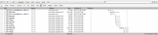
Figure 2-5. Filtering results by resource type

Generally you can use Firebug to get an idea of potential issues either during development or for production support. You can proactively monitor the size of your payloads and the general load time, and you can check to make sure that your pages aren’t taking too long to load. What is the overall size of my page, what are the largest assets, and what is taking the longest to load? You can answer questions like that. You can use the filters to focus on areas of concern, like seeing how large our external JavaScript files are. Or even sort the rows by domain name to see content grouped by domain, or sort by HTTP status to quickly pick out any calls that are erroring out.

Because Firebug is a passive tool that merely reports what is happening and doesn’t give recommendations for improvements, it’s best suited as a development tool or for debugging issues that arise.

YSlow

For a deeper analysis of a page’s web performance you can use YSlow.

Developed by Steve Souders and the team at Yahoo!, YSlow was released in 2007. It was initially released as a Firefox extension, but eventually it was ported to work with most other browsers as well. Like Firebug, YSlow is an in-browser tool, and like Firebug it does not allow much automation, but it is an invaluable tool to assess a page’s web performance and get feedback on steps to take to improve performance.

The steps for improvement are what really distinguish YSlow. It uses a set of criteria to evaluate the performance of a given page and gives feedback that is specific to the needs of your site. Best of all, the criteria are a living thing, and the YSlow team updates them as best practices change and old ones become less relevant.

Let’s try out YSlow.

How to Install

To install YSlow, simply navigate to http://yslow.org/ and choose the platform that you want to run it in. Figure 2-6 shows all the different browsers and platforms that are currently available on the YSlow website.

Since we are already using Firefox with Firebug, let’s continue to use that browser for YSlow. Once you select the Firefox version, install the extension and restart the browser, you are ready to start using YSlow.

Figure 2-6. Different ways to access YSlow

How to Use

In Firefox if you open up Firebug you can see that it has a new tab called YSlow. When you click on the tab you are presented with the splash screen shown in Figure 2-7. From this screen you can run the YSlow test on the page that is currently loaded in the browser or choose to always run the test whenever a new page is loaded.

You can also choose what rule set to have the page evaluated against, As I’ve been saying, best practices change, and the different rule sets reflect that. There is the classic set of rules that YSlow initially launched with, an updated rule set (V2) that changed the weighting of certain rules (like making CSS and JavaScript external) and added a number of new rules, and a subset of the rules for small-scale sites and blogs where those rules would be overkill.

After running the test you’ll see the results screen shown in Figure 2-8. The results screen is split into two sections: the rules with their respective ratings on the left and an explanation of the rule on the right.

For a detailed breakdown of the rules that YSlow uses, see http://developer.yahoo.com/performance/rules.html.

There is a sub-navigation bar that further breaks down the results, showing the page components, statistics for the page, and tools you can use for further refinement of performance.

The components section is much like the Network Monitoring tab in Firebug; it lists the individual assets in the page, and each component’s file size, URL, response header, response time, expires header, and etag.

Figure 2-7. The YSlow extension

Figure 2-8. The YSlow results screen

But beware; etags are unique to the server that generated them. If your content is being served by a cluster, that is an array of servers, rather than a single server. The etags won’t match if a client requests the content from a different server, and you won’t get the benefit of having the content cached.

The statistics section, shown in Figure 2-9, displays two pie charts that show the breakdown of page components. The left chart shows the results with no content cached, and the right shows a subsequent cached view. This is useful to identify the areas that can give the biggest improvement.

By comparing the two charts in Figure 2-9, you can see that JavaScript and images are the two largest pieces of the page before caching. Caching alleviates this for images, but I bet we can get our JavaScript footprint even lower by using a tool that we’ll be talking about soon, Minify.

There are other products similar to YSlow. Google has since made available Page Speed, as a standalone site located here: https://developers.google.com/speed/pagespeed/insights. Page Speed is also available as a browser extension for Chrome or Firefox, available here: https://developers.google.com/speed/pagespeed/insights_extensions.

The differences between YSlow and Page Speed are negligible, and subject to personal preferences in style and presentation.

Figure 2-10 shows the results of a Page Speed test run in the developer tools in Chrome.

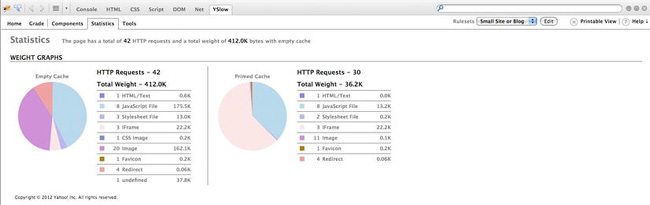
Figure 2-9. The YSlow results screen—statistics

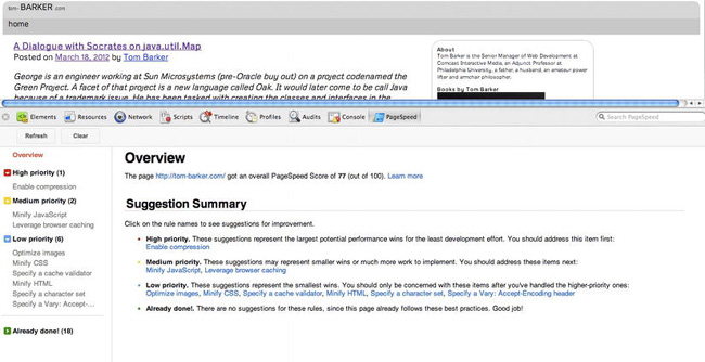
Figure 2-10. Page Speed results

Another similar product is WebPagetest. Because of its rich feature set and potential automation, WebPagetest will be the next product that we talk about at length.

WebPagetest

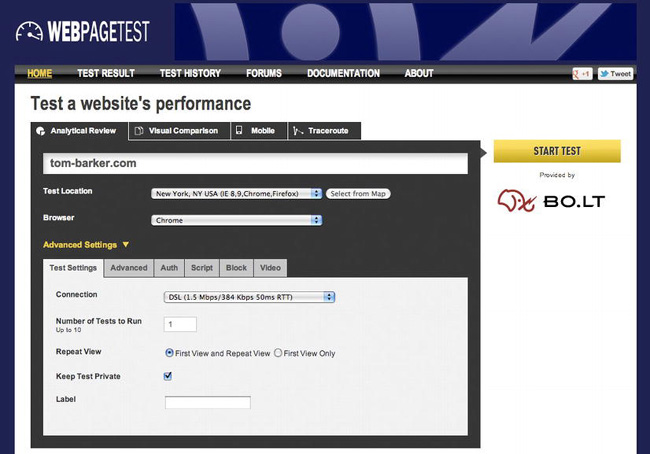
WebPagetest was originally created by AOL and open sourced for public consumption and contribution in 2008. It is available as a public web site, as an open source project, or for download to run a private instance. The code repository is found at http://code.google.com/p/webpagetest/. The public web site is located at http://www.webpagetest.org/ and can be seen in Figure 2-11. The public site is maintained and run by Pat Meenan, through his company WebPagetest LLC.

WebPagetest is a web application that takes a URL and a set of configuration parameters as input and runs performance tests on that URL. The number and range of parameters that we can configure for WebPagetest is extraordinarily robust.

If you want to run tests on web sites that are not publicly available—like a QA or development environment, or if you can only have your test results stored on your own servers because of legal or other reasons, then installing your own private instance of WebPagetest is the way to go.

Otherwise, there is no reason not to use the public instance.

You can choose from a set of locations from around the world where your tests can be run. Each location comes with one or more browsers that can be used for the test at that location. You can also specify the connection speed and the number of tests to run.

In the Advanced panel, you can have the test stop running at document completion. That will tell us when the document.onload event is fired, instead of when all assets on the page are loaded. This is useful because XHR communications that may happen after page load could register as new activity and skew the test results.

You can also have the test ignore SSL certification errors that would otherwise block the test because an interaction with the end user would be needed to either allow the transaction to proceed, view the certificate, or cancel the transaction.

Figure 2-11. Webpagetest.org

There are a number of other options in the Advanced tab; you can have the test capture the packet trace and network log, providing the granular details of the network transactions involved in the test, or select the “Preserve original User Agent string” option to have the test keep the user agent string of the browser running the test instead of appending a string to identify the visit as a WebPagetest test.

In the Auth tab you can specify credentials to use if the web site uses HTTP authentication for access; just remember to exercise caution. Using real production usernames and passwords for tests staged and stored on public servers is never recommended. It is much more advisable to create test credentials for just this purpose, with constrained permissions.

Sometimes you need to test very specific conditions. Maybe you are running a multivariate test on a certain feature set where you are only serving specific features on specific client configurations, like iPhone specific features. Or you are targeting certain features for users that are grouped by inferred usage habits. You would want to run performance tests on these features that are only triggered by special events.

The Script tab allows you to do just that. You can run more complex tests that involve multiple steps including navigate to multiple URLs, send Click and Key events to the DOM, submit form data, execute ad hoc JavaScript, and update the DOM. You can even alter the HTTP request settings to do things like set specific cookies, set the host IP, or change the user agent.

For example, to make a client appear to be an iPhone, simply add the following script:

The setUserAgent command spoofs the client user agent, and the navigate command points the test to the specified URL. You can read more about the syntax and some of the great things you can do with scripting WebPagetest here: https://sites.google.com/a/webpagetest.org/docs/using-webpagetest/scripting.

The Block tab allows us to block content coming in our request. This is useful to compare results with and without ads, with or without JavaScript, and with or without images. Instead of using the block tab we could just incorporate a blocking command as part of our script in the Script tab. If we wanted to script out blocking all PNGs in a site it would look like this:

And finally, the Video tab allows you to capture screen shots of your page as it loads and view them as a video. This is useful for being able to see what a page looks like as it loads, particularly when you have content loaded in asynchronously; you can see at what point in the process the page looks to be usable.

So once you’ve set all of the configuration choices, you can run the test. You can see my results screen in Figure 2-12.

Figure 2-12. The webpage test results page

First the Summary screen aggregates all of the vital relevant information for you. At the top right is a summary of the Page Speed results for our page. This is a high-level representation of the same information that would be presented if we had run a test in Page Speed, but shown in YSlow’s letter grading format.

Sitting in a table above the waterfall charts and screen shots are the page level metrics, numbers for the load time of the full page, how long the first byte took to load, how long until the first piece of content was drawn to the stage, how many DOM elements are on the page, the time it took for the document.onload event to fire, the time it took for all elements on the page to load, and the number of HTTP requests were needed to draw the page.

Make note of these data. They comprise the fundamental information that makes up the quantitative metrics that you will use to chart web performance in the next chapter. They are the true essence of a site’s web performance.

Below this table are two columns. On the left are waterfall charts for the first-time view and the cached repeat view, and on the right are the corresponding screen shots. We’ve already talked at length about how useful waterfall charts are.

Below these are two pie charts. The chart on the left shows the percent of requests by content type. The chart on the right shows the percent of bytes by content type, which is useful for identifying the largest areas that can be optimized. If your JavaScript is only 5% of your overall payload but your images are 70%, you would be better served optimizing images first.

This summary page aggregates at a high level all of the data that you can find in the pages accessed by its sub-navigation bar. Click on the Details, Performance Review, Page Speed, Content Breakdown, Domains, and Screen Shot links in this bar for a deeper dive into each. The Content Breakdown section can be seen in Figure 2-13. This shows how each piece of content fares in the criteria outlined in the column names (Keep-Alive, Gzip text, Compress Images, Cache Static, Combine, CDN detected, Minify JS, and cookies). The green check marks indicate a success in the criteria, the yellow triangles with the exclamation points indicate a warning, and the red Xs indicate errors.

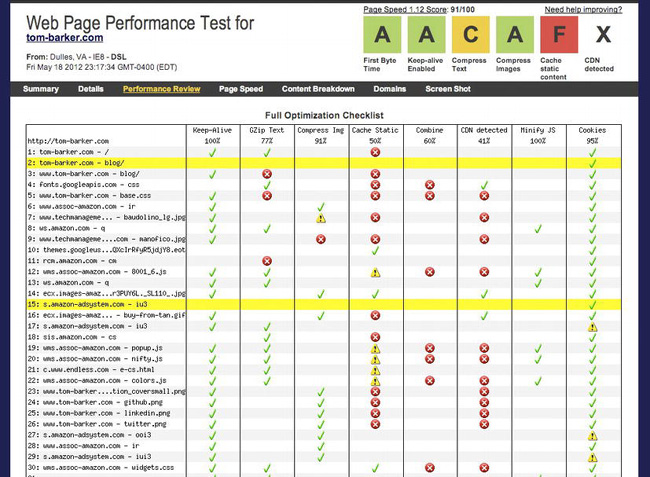
Figure 2-13. The Webpagetest performance optimization checklist

As you can see, WebPagetest provides a wealth of information about the web performance of a site, but best of all it’s fully programmable. It provides an API that you can call to provide all of this information. Next chapter we’ll explore the API and construct our own application for tracking and reporting out web performance.

Minification

In general, a good amount of energy is spent thinking about optimizing caching. This is a great thing because caching as much content as you can will both create a better user experience for subsequent visits and save on bandwidth and hits to your origin servers.

But when a user comes to a site for the first time there will be no cache. So to ensure that our first-time visits are as streamlined as possible, we need to minify our JavaScript.

Minification is originally based on the idea that the JavaScript interpreter ignores white space, line breaks, and of course comments, so we can save on total file size of our .js files if we remove those unneeded characters.

There are many products that will minify JavaScript. Some of the best ones add twists on that concept.

Minify

First we’ll look at Minify, available at http://code.google.com/p/minify/. Minify proxies the JavaScript file; the script tag on the page points to Minify, which is a PHP file (In the following code we point to just the /min directory because the PHP file is inde.php). The script tag looks like this:

Minify reads the JavaScript file in, minifies it and when it responds it sets the accept encoding HTTP header to gzip, deflate. Effectively it has built in HTTP static compression. This is especially useful if your web host doesn’t allow the gzipping of static content (like the web host I use, unfortunately). See the high level architecture of how Minify works in Figure 2-14.

To use Minify, simply download the project from http://code.google.com/p/minify/, place the decompressed /min folder in the root of your web site, and navigate to the Minify control panel, located at /min/builder/.

From this control panel you can add the JavaScript files you want included in the minified result, and the page generates the script tag that you can use to link to this result. Fairly simple.

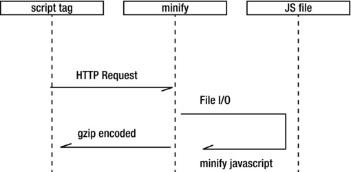
Figure 2-14. Sequence diagram for Minify. The script tag points to Minify, passing in the URL of the JavaScript file. Minify strips out unneeded characters, sets the response header to be gzip-encoded, and returns the result to the script tag, which loads in the browser.

YUI Compressor

Another minification tool is Yahoo’s YUI Compressor, available here: http://yuilibrary.com/download/yuicompressor/. YUI Compressor is a jar file and runs from the command line. Because of this it is easily integrated into a build process. It looks like this:

Just like Minify, YUI Compressor strips out all of the unnecessary characters from your JavaScript, including spaces, line breaks, and comments. For a more detailed look at the options available for YUI Compressor, see http://developer.yahoo.com/yui/compressor.

Closure Compiler

Finally we’ll look at Google’s Closure Compiler, available at https://developers.google.com/closure/compiler/. Closure Compiler can also run from the command line and be built into an automated process, but it takes minification one step further by rewriting as well as minifying the JavaScript. To rewrite our JavaScript, Closure Compiler runs through a number of “scorched-earth” optimizations—it unfurls functions, rewrites variable names, and removes functions that are never called (as far as it can tell). These are considered “scorched-earth” optimizations because they strip everything out, including best practices, in search of the leanest payload possible. And the approach succeeds. We would never write our code in this way, so we keep our originals, and run them through Closure Compiler to “compile” them into the most optimized code possible. We keep this “compiled” code as a separate file, so that we have our originals to update.

To get an idea of how Closure Compiler rewrites our JavaScript, let’s look at some code before and after running Closure Compiler. For the “before” we’re using a small code example that we will be using in Chapter 7.

Closure Compiler takes that code and rewrites it as this:

It’s a significant improvement in all performance metrics, but at the cost of readability, and abstraction from the original code.

Comparison of Results

To determine the best tool to use for a given situation, we’ll take the scientific approach! Let’s implement the tools just discussed and run a multivariate test to see for ourselves which will give us the best results.

First we’ll look at a waterfall chart of a sample of unminified code, as seen in Figure 2-15.

We see that uncompressed and unminified our JavaScript file is 2.1 KB and our total page size is 3.3KB. This sample can be found at http://tom-barker.com/lab/perfLogger_example.html.

Now let’s use Minify and test those results. You can see in the waterfall chart from Figure 2-16 that the JavaScript served from Minify (both minified and gzipped) is only 573 bytes, and the total page size is 1.9 KB.

When I use YUI Compressor and Closure Compiler (with simple options chosen, so the file is only minified, not rewritten) on these same files I get the same result; the JavaScript file is reduced to 1.6 KB for each and the total page size is 2.9 KB. See Figure 2-17.

Remember, the web host that I am using does not support HTTP compression at a global scale, so these results are simply minified, not gzipped. Thus these are not apples-to-apples comparison of the minification algorithm, just a comparison of using the products out of the box.

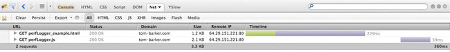
Figure 2-15. Waterfall chart with uncompressed JavaScript, our baseline

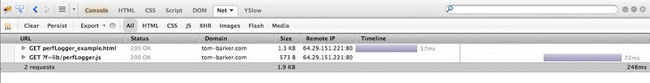
Figure 2-16. The page compressed with Minify

Figure 2-17. The page compressed with Closure Compiler (simple)

Figure 2-18. The page compressed and included in-line with Closure Compiler (advanced)

The final comparison is to take the original JavaScript file and run it through Closure Compiler with the Advanced option enabled, so it rewrites the code to be as streamlined as possible. When you do this, make sure you include all JavaScript on the page; that is, not just the remote js file, but also the JavaScript on the page that instantiates the objects. It’s necessary to do this because Closure Compiler will eliminate all code that it does not see executed. So if you have a namespaced object in a remote JS file but code to instantiate it on the HTML page, you need to include the code that instantiates the object in the same file so Closure Compiler can see that it’s used and include it in its output.

The final output from Closure Compiler I will embed on the HTML page instead of linking to it externally. You can see the results in Figure 2-18.

Now that we have some data, let’s visualize it and evaluate.

Analysis and Visualization

We’ll open up R and pour in our minification results, the tool names, the new file size for each tool’s output, and the percent difference for each. We’ll then code some R to create a horizontal bar chart to compare the difference.

Don’t worry, to do this we’ll explore R in depth, and when we do I’ll explain what each line does. For now let’s roll with it and look at the chart you’ll ultimately generate, shown in Figure 2-19.

You can see from Figure 2-19 that Closure Compiler gives the greatest reduction in size right out of the box, but Minify’s combination of minification and gzipping brings it in to a close second. YUI and the simple minification that Closure Compiler provide come in tied a distant third.

Again this comparison is performance out of the box—if we had gzipped our results at third place they would have had comparable results to Minify’s, but Minify supplies gzipping out of the box.

Sheer file size reduction is only one aspect of our overall determination. As you saw in the example earlier, Closure Compiler’s advanced output is far different from the code that originally went into it. If issues were to arise in production they could be difficult to debug, especially if there is third-party code on your pages interacting with your own code.

Does your site have third-party code, like ad code? Are you hosting your own servers or beholden to a web host? How important is production support to you, compared to having the absolute fastest experience possible? When determining your own preferred tool, it is best to evaluate as we just did and see what works best for your own situation, environment, and business rules. For example, do you have a build environment where you can integrate this tool and have control over configuring your web host? If so, then YUI or Closure Compiler might be your best choices. Are you comfortable with the scorched-earth approach of Closure Compiler’s advanced setting? If so, that gives the greatest performance boost – but good luck trying to debug its output in production.

Figure 2-19. Comparison chart generated in R to show percent of file reduction by product

Getting Started with R

R was created in 1993 by Ross Ihaka and Robert Gentleman. It is an extension of and successor to the S language, which was itself a statistical language created in 1976 by John Chambers while at Bell Labs.

R is both an open source environment and the language that runs in that environment, for doing statistical computing. That’s a very general description. I’m not a statistician, nor am I a data analyst. I’m a web developer and I run a department of web developers, if you are reading this, chances are you are a web developer. So what do we, as web developers, do with R?

Generally I use R to suck in data, parse it, process it, and then visualize it for reporting purposes. Figure 2-20 illustrates this workflow. It’s not the only language I use in this workflow, but it is my new favorite. I need other languages usually to access a data source or scrape another application. In the next chapter we use PHP for this, our glue language, but we could use almost any other language—Ruby, shell script, Perl, Python, and so on.

After I use a glue language to collect the data, I write the data out as a comma-separated file, and read it into R. Within R I process the data, splitting it, averaging it, aggregating it, overlaying two or more data sets, and then from within R I chart the data out to tell the story that I see in it.

Once I have a chart created, generally as a PDF so that it maintains its vectors and fonts, from R I import the chart into Adobe Illustrator, or any other such program, where I can clean up things like font consistency and make sure axis labels with long names are visible.

Figure 2-20. Workflow for preparing data visualizations with R

What kinds of data do I run in R? All kinds. In this book we look at visualizing performance data in R, but I also report on my departmental metrics using R, things like defect density, or code coverage for my code repositories.

As a language it is small, self-contained, extensible, and just fun to use. That said, it does have its own philosophy, and quirks, some of which we’ll look at here.

Installing and Running R

To install R, you first need to download a precompiled R binary, from http://cran.r-project.org/. For Mac and PC, this is a standard installer that walks you through the installation process. The PC installer comes in three flavors: Base is the base install, Contrib comes with compiled third-party packages, and Rtools comes with tools to build your own R packages. For our purposes we’ll stick with the base install. See Figure 2-21 for a screen shot of the R installer.

Instead of a compiled installer, Linux users get the command sequence to install for their particular Linux flavor.

Once R is installed, you can open the R Console, the environment from which we will run the R language. The console can be seen in Figure 2-22.

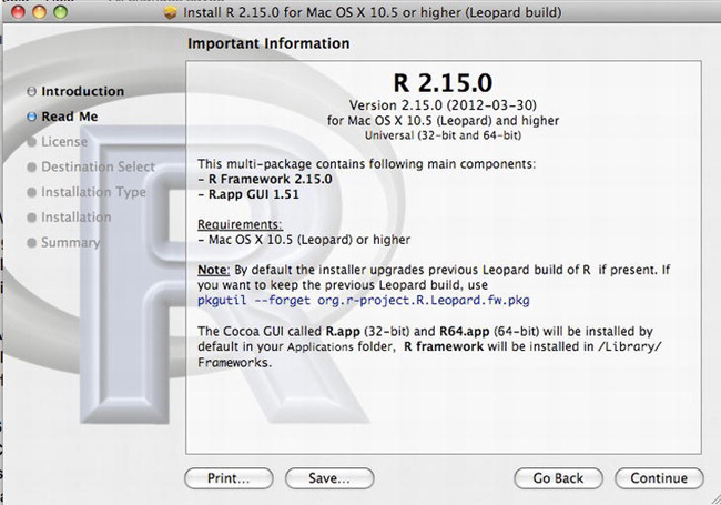
Figure 2-21.R installer for Mac

Figure 2-22. The R console

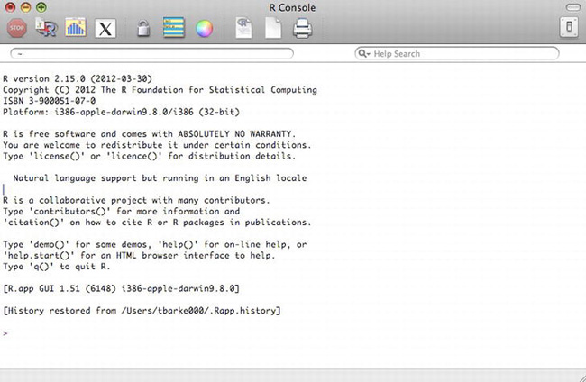
The console’s toolbar allows us to do tasks like interrupt the execution of running R processes, run stand-alone .R files, adjust the look and feel of the console, create new stand-alone .R files, and so on.

The R Console is a command-line environment for running ad hoc R commands. Usually I use the console to flesh out ideas, and tweak them until they produce what I am looking for, and then I move those functioning expressions to a standalone R file.

You can create external files to hold your R code, generally they have the extension .R.

R is also highly extensible and has a robust community that builds packages that extend what can be done with R. That said, for all of the R code in this book we will not be using any packages, sticking only to the base install of R.

An R Primer

Now that you understand what R is, how do you use R? The first things to note are that at any time you can type ?[keyword] to open the help window for a particular subject. If you aren’t sure that what you are looking for has a topic, simply type ??[keyword] to do a more extensive search. For example, type ?hist to search for help on creating histograms.

Also important to note is that R supports single-line comments, but not multiline comments. The hash symbol starts a comment, and the R interpreter ignores everything after the hash symbol to the line break.

Variables and Data Types

To declare a variable you simply assign value to it. The assignment operator is a left-pointing arrow, so creating and declaring variables looks like this:

R is loosely typed, and it supports all of the scalar data types you would expect: string, numbers, and booleans.

It also supports lists, but here is one of the quirks of the language. R has a data type called vector that functions almost like a strictly typed single-dimensional array. It is a list whose items are the same data type, either strings, numbers, or booleans. To declare vectors use the combine function c(), and you add to vectors with the c() function as well. You access elements in vectors using square brackets. Unlike arrays in most languages, vectors are not zero based; the first element is referenced as element [1].

R also has another list type, called matrix. Matrices are like strictly typed two dimensional arrays. You create a matrix using the matrix function, which accepts five parameters: a vector to use as the content, the number of rows to shape the content into, the number of columns to shape the content into, an optional boolean value to indicate whether the content should be shaped by row or by column (the default is FALSE for by column), and a list that contains vectors for row names and column names:

You access indexes in a matrix with square brackets as well, you we must specify the column and the row in the square brackets.

So far both matrices and vectors can only contain a single data type. R supports another list type, called a data frame. Data frames are multidimensional lists that can contain multiple data types—sort of. It is easier to think of data frames as collections of vectors. Vectors still have to hold only one data type, but a data frame can hold multiple types of vectors.

You create data frames using the data.frame() function, which accepts a number of vectors as content, and then the following parameters: row.names to specify the vector to use as row identifiers, check.rows to check consistency of row data, and check.names to check for duplicates among other syntactical checks.

Use square brackets to access individual vectors within data frames:

Use the $ notation to isolate columns, and the square bracket for individual indexes of those columns. The $ in R is much like dot notation in most other languages.

Importing External Data

Now that you’ve seen how to hold data, let’s look at how to import data. You can read data in from a flat file using the read.table() function. This function accepts four parameters: the path to the flat file to read in, a boolean to indicate whether the first row of the flat file contains header names or not, the character to treat as the column delimiter, and the column to treat as the row identifier. The read.table() function returns a data frame.

For example, suppose you have the following flat file, which has a breakdown of a bug backlog:

You would read this in with the following code:

If you examine the resulting bugData object, you should see the following:

Loops

R supports both for loops and while loops, and they are structured much as you would expect them to be:

To loop through the users data frame, you can simply do the following:

The same applies for the bug data:

Functions

Functions in R also work as you would expect; we can pass in arguments, and the function accepts them as parameters and can return data out of the function. Note that all data is passed by value in R.

We construct functions in this way:

Simple Charting with R

Now here is where things start to get really fun with R. You know how to import data, store data, and iterate through data; let’s visualize data!

R natively supports several charting functions. The first we will look at is plot().

The plot() function will display a different type of chart depending on the arguments that you pass in to it. It accepts the following parameters: an R object that supports the plotting function, an optional parameter that will supplement as a y axis value in case the first parameter does not include it, the number of named graphical parameters, a string to determine the type of plot to draw (more on this in a second), the title of the chart, a subtitle of the chart, the label for the x-axis, the label for the y-axis, and finally a number to indicate the aspect ratio for the chart (the aspect ratio is the numeric result of y/x).

Let’s take a look at how some of the plot type options are reflected in the display of the chart. Note that when you plot the users data frame, you get a numeric representation of the user names column on the x-axis and the y-axis is the admin column, but shown in a range from 0 to 1 (instead of TRUE and FALSE). Figure 2-23 shows the results.

Bar charts are also supported in the base installation of R, with the barplot() function. Some of the most useful parameters that the barplot() function accepts are a vector or matrix to model the height of the bars, an optional width parameter, the amount of space that will precede each bar, a vector to list as the names for each bar, the text to use as the legend, a boolean value named beside that signifies whether the bar chart is stacked, another boolean value set to true if the bars should be horizontal instead of vertical, a vector of colors to use to color the bars, a vector of colors to use as the border color for each bar, and the header and sub header for the chart. For the full list simply type ?barplot in the console.

Figure 2-24 shows what the users data frame looks like as a bar chart.

You can also create bubble charts natively in R. To do this, use the symbols() function, pass in the R object that you want to represent, and set the circles parameter to a column that represents the radius of each circle.

Figure 2-25 shows the result.

Figure 2-23. The different types of chart with the plot function

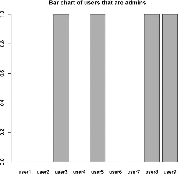
Figure 2-24. Bar chart of users that are admins

Figure 2-25. Bubble chart of users that are admins

The symbols() function can be used to draw other shapes on a plot; for more information about this type ?symbols at the R console.

You can save the charts that you generate by calling the appropriate function for the file type you want to save. Note that you need to call dev.off after you are done outputting. So, for example, to create a JPEG of the barplot you would call:

The functions available are these:

A Practical Example of R

This has been just the barest taste of R, but now that you understand its basic building blocks, let’s construct the chart that you saw in Figure 2-19 earlier.

First you’ll create four variables, one a number to hold the value of the uncompressed JavaScript file, one a vector to hold the names of the tools, one a vector to hold the file size of the JavaScript files after they have been run through the tools, and a final vector to hold the percentage difference between the minified size and the original size.

You’ll be refactoring that last variable soon, but for now leave it hard-coded so you can see the pattern that we are applying to gather the percentage—100 minus the result of the new size divided by the total size multiplied by 100.

Next create a data frame from those vectors, and make the row identifier the vector of tool names.

If you type mincompare in the console, you’ll see that it is structured like this:

Perfect! From here you can start to construct the chart. Use the barplot function to plot the diff column. Make the chart horizontal, explicitly set the y-axis names to the row names of the data frame, and give the chart a title of “Percent of file size reduction by product”:

If you run this in the console you’ll see that we’re almost there. It should look like Figure 2-26.

You can see that the first and third y-axis names are missing; that’s because the copy is too large to fit vertically as it is now. You can correct this by making the text horizontal just like the bars are.

To do this, set the graphical parameters of the chart using the par function. But first, save the existing parameters so that you can revert back to them after creating the chart:

This saves the existing parameters in a variable called opar so you can retrieve them after you are done.

Next you can make the text horizontal, with the par() function:

Figure 2-26. First draft of chart

The par() function accepts several parameters. This code passes in the las parameter (to alter the axis label style) and sets it to 1, which makes the axis labels always horizontal, and passes in the mar parameter to set the margins for the chart.

After you call barplot to draw the chart, you can then revert to the original graphical parameters, with this code:

To save this chart you need to export it. You can wrap the barplot and par calls in a call to the pdf function, passing in the file name to save the chart with. This example will export as a PDF to retain the vector lines and raw text so that we can edit and refine those things in post-production using Illustrator or some other such program:

After restoring the graphical parameters, close the file by calling dev.off()

So far the code should look like this:

But something about this bothers me. I don’t like having our diff variable hard-coded, and we’re repeating the algorithm over and over again to set the values. Let’s abstract that out into a function.

Call the function getPercentImproved and have it accept two parameters, a vector of values and a number value:

Within the function, create an empty vector; this will hold the results of our function and we will return this vector at the end of the function:

Then loop through the passed-in vector:

Within the iteration we run our algorithm to get the difference between the numbers in each element. Remember, it’s

(100–([new file size] /[original file size])*100)

Save the result of this in our new vector percentVector:

And after the loop completes we’ll return the new vector.

Our final function should look like this:

Finally, set the vector diff to be the result of getPercentImproved, and pass in the vector called size and the variable originalSize;

Your final code should look like this:

There are many ways to further refine this if you wanted. You could abstract the generating and exporting of the chart to a function.

Or you could use a native function of R called apply() to derive the difference instead of looping through the vector. Let’s take a look at that right now.

Using apply()

The apply() function allows us to apply a function to elements in a list. It takes several parameters; first is a list of values, next a number vector to indicate how we apply the function through the list (1 is for rows, 2 is for columns, and c(1,2) indicates both rows and columns), and finally the function to apply to the list:

We could eliminate the getPercentImproved function and instead use the following:

Note that this converts the size variable into a matrix as we pass it to apply(). This is because apply() expects matrices, arrays, or data frames. The apply() function has a derivative lapply() that you could use as well.

When using apply your code is smaller, and it uses the language as it was intended, it adheres to the philosophy of the language, meaning that it is more about logical programming with statistical analysis than imperative programming. The updated code should now look like this:

The final step to constructing the chart would be to bring it into Adobe Illustrator or some other vector painting program to refine it, for example adjusting the alignment of text or the size of fonts. While this kind of formatting is possible within R, it is much more robust in a dedicated application.

Summary

In this chapter we learned about several tools that are invaluable to us in our goal to create and maintain performant web sites. We saw how Firebug’s Network Monitoring tab is a great tool to keep track of the network dependencies that make up our pages and the impacts that they have on our page speed. Its passive nature makes Network Monitoring a great tool to use as we develop pages or debug known issues.

We used the different filters with YSlow to test the current performance of our sites, but also to get customized tips to better optimize the web performance of these sites.

With Webpagetest we were also able to see the impact of external assets and get performance tips, but we were then able to see the results of repeat viewing, and get high level aggregate data for several different aspects of data as well. We saw the robust configuration set that WebPagetest sports, including scripting capabilities to test more complex scenarios. We also saw that WebPagetest exposes an API, we will use that next chapter to automate performance monitoring.

We explored several tools for minifying our JavaScript. We implemented each tool and compared the results by visualizing the differences in file size that each tool gave us. We also started to look at some of the abstract details that make performance about more than just the numbers.

We then dipped our toes in the R language. We installed the R console, explored some introductory concepts in R, and coded our first chart in R—the same chart that we used to compare the results of the minification tool comparison.

In the coming chapters we will use and expand on our knowledge of R, as well as make use of many of the tools and concepts that we explored this chapter.