I now turn to using SAS Enterprise Miner to derive and interpret neural network models. This chapter develops two neural network models using simulated data. The first model is a response model with a binary target, and the second is a risk model with an ordinal target.

5.1.1 Target Variables for the Models

The target variable for the response model is RESP, which takes the value of 0 if there is no response and the value of 1 if there is a response. The neural network produces a model to predict the probability of response based on the values of a set of input variables for a given customer. The output of the Neural Network node gives probabilities Pr(RESP=0|X) $\Pr (R E S P = 0 | X)$ and Pr(RESP=1|X) $\Pr (R E S P = 1 | X)$ , where X $X$ is a given set of inputs.

The target variable for the risk model is a discrete version of loss frequency, defined as the number of losses or accidents per car-year, where car-year is defined as the duration of the insurance policy multiplied by the number of cars insured under the policy. If the policy has been in effect for four months and one car is covered under the policy, then the number of car-years is 4/12 at the end of the fourth month. If one accident occurred during this four-month period, then the loss frequency is approximately 1/ (4/12) = 3. If the policy has been in effect for 12 months covering one car, and if one accident occurred during that 12-month period, then the loss frequency is 1/ (12/12) = 1. If the policy has been in effect for only four months, and if two cars are covered under the same policy, then the number of car-years is (4/12) x2. If one accident occurred during the four-month period, then the loss frequency is (1 / (8/12) = 1.5. Defined this way, loss frequency is a continuous variable. However, the target variable LOSSFRQ, which I will use in the model developed here, is a discrete version of loss frequency defined as follows:

L O S S F R Q = 0 i f l o s s f r e q u e n c y = 0, L O S S F R Q = 1 i f 0 < l o s s f r e q u e n c y < 1.5, a n d L O S S F R Q = 2 i f l o s s f r e q u e n c y \geq 1.5.

$\begin{array}{l} L O S S F R Q = 0 i f l o s s f r e q u e n c y = 0, \\ L O S S F R Q = 1 i f 0 < l o s s f r e q u e n c y < 1.5, a n d \\ L O S S F R Q = 2 i f l o s s f r e q u e n c y \geq 1.5. \end{array}$

The three levels 0, 1, and 2 of the variable LOSSFRQ represent low, medium, and high risk, respectively.

The output of the Neural Network node gives:

Pr (L O S S F R Q = ​ ​ ​ ​ ​ ​ 0 | X) = Pr (l o s s f r e q u e n c y = 0 | X), Pr (L O S S F R Q = 1 | X) = Pr (0 < l o s s f r e q u e n c y < 1.5 | X), Pr (L O S S F R Q = ​ 2 | X) = Pr (l o s s f r e q u e n c y \geq 1.5 | X) .

$\begin{array}{l} \Pr (L O S S F R Q = 0 | X) = \Pr (l o s s f r e q u e n c y = 0 | X), \\ \Pr (L O S S F R Q = 1 | X) = \Pr (0 < l o s s f r e q u e n c y < 1.5 | X), \\ \Pr (L O S S F R Q = 2 | X) = \Pr (l o s s f r e q u e n c y \geq 1.5 | X) . \end{array}$

5.1.2 Neural Network Node Details

Neural network models use mathematical functions to map inputs into outputs. When the target is categorical, the outputs of a neural network are the probabilities of the target levels. The neural network model for risk (in the current example) gives formulas to calculate the probability of the variable LOSSFRQ taking each of the values 0, 1, or 2, whereas the neural network model for response provides formulas to calculate the probability of response and non-response. Both of these models use the complex nonlinear transformations available in the Neural Network node of SAS Enterprise Miner.

In general, you can fit logistic models to your data directly by first transforming the variables, selecting the inputs, combining and further transforming the inputs, and finally estimating the model with the original combined and transformed inputs. On the other hand, as I show in this chapter, these combinations and transformations of the inputs can be done within the neural network framework. A neural network model can be thought of as a complex nonlinear model where the tasks of variable transformation, composite variable creation, and model estimation (estimation of weights) are done simultaneously in such a way that a specified error function is minimized. This does not rule out transforming some or all of the variables before running the neural network models, if you choose to do so.

In the following pages, I make it clear how the transformations of the inputs are performed and how they are combined through different “layers” of the neural network, as well as how the final model that uses these transformed inputs is specified.

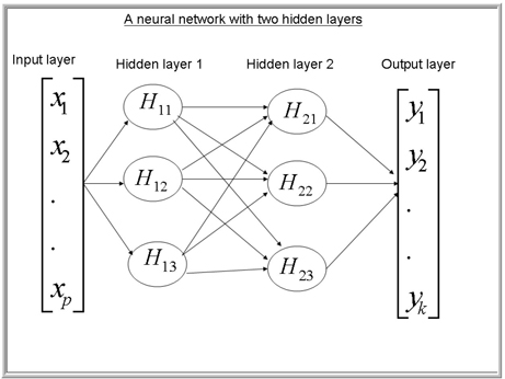
A neural network model is represented by a number of layers, each layer containing computing elements known as units or neurons. Each unit in a layer takes inputs from the preceding layer and computes outputs. The outputs from the neurons in one layer become inputs to the next layer in the sequence of layers.

The first layer in the sequence is the input layer, and the last layer is the output, or target, layer. Between the input and output layers there can be a number of hidden layers. The units in a hidden layer are called hidden units. The hidden units perform intermediate calculations and pass the results to the next layer.

The calculations performed by the hidden units involve combining the inputs they receive from the previous layer and performing a mathematical transformation on the combined values. In SAS Enterprise Miner, the formulas used by the hidden units for combining the inputs are called Hidden Layer Combination Functions. The formulas used by the hidden units for transforming the combined values are called Hidden Layer Activation Functions. The values generated by the combination and activation operations are called the outputs. As noted, outputs of one layer become inputs to the next layer.

The units in the target layer or output layer also perform the two operations of combination and activation. The formulas used by the units in the target layer to combine the inputs are called Target Layer Combination Functions, and the formulas used for transforming the combined values are called Target Layer Activation Functions. Interpretation of the outputs produced by the target layer depends on the Target Layer Activation Function used. Hence, the specification of the Target Layer Activation Function cannot be arbitrary. It should reflect the business question and the theory behind the answer you are seeking. For example, if the target variable is response, which is binary, then you should select Logistic as the Target Layer Activation Function value. This selection ensures that the outputs of the target layer are the probabilities of response and non-response.

The combination and activation functions in the hidden layers and in the target layer are key elements of the architecture of a neural network. SAS Enterprise Miner offers a wide range of choices for these functions. Hence, the number of combinations of hidden layer combination function, hidden layer activation function, target layer combination function, and target layer activation function to choose from is quite large, and each produces a different neural network model.

5.2 A General Example of a Neural Network Model

To help you understand the models presented later, here is a general description of a neural network with two hidden layers¹ and an output layer.

Suppose a data set consists of n $n$ records, and each record contains, along with a person’s response to a direct mail campaign, some measures of demographic, economic, and other characteristics of the person. These measures are often referred to as explanatory variables or inputs. Suppose there are p $p$ inputs xi1,xi2,.....xip $x_{i 1}, x_{i 2}, ..... x_{i p}$ for the ith $i^{t h}$ person. In a neural network model, the input layer passes these inputs to the next layer. In the input layer, there is one input unit for each input. The units in the input layer do not make any computations other than optionally standardizing the inputs. The inputs are passed from the input layer to the next layer. In this illustration, the next layer is the first hidden layer. The units in the first hidden layer produce intermediate outputs. Suppose there are three hidden units in this layer. Let Hi11 $H_{i 11}$ denote the intermediate output produced by the first unit of the first hidden layer for the ith $i^{t h}$ record. In general, Hikj $H_{i k j}$ stands for the output of the jth $j^{t h}$ unit in the kth $k^{t h}$ hidden layer for the ith $i^{t h}$ record in the data set.

Similarly, the intermediate outputs produced by the second and third units are Hi12 $H_{i 12}$ and Hi13 $H_{i 13}$ . These intermediate outputs are passed to the second hidden layer. Suppose the second hidden layer also contains three units. The outputs of these three hidden units are Hi21 $H_{i 21}$ , Hi22 $H_{i 22}$ and Hi23 $H_{i 23}$ . These intermediate outputs become inputs to the output or target layer, the last layer in the network. The output produced by this layer is the predicted value of the target, which is the probability of response (and non-response) in the case of the response model (a binary target), and the probability of the number of losses occurring in the case of the risk model (an ordinal target with three levels). In the case of a continuous target, such as value of deposits in a bank or household savings, the output of the final layer is the expected value of the target.

In the following sections, I show how the units in each layer calculate their outputs.

The network just described is shown in Display 5.0A.

Display 5.0A

5.2.1 Input Layer

This layer passes the inputs to the next layer in the network either without transforming them or, in the case of interval-scaled inputs, after standardizing the inputs. Categorical inputs are converted to dummy variables. For each record, there are p $p$ inputs: x1,x2,........xp $x_{1}, x_{2,} ........ x_{p}$ .

5.2.2 Hidden Layers

There are three hidden units in each of the two hidden layers in this example. Each hidden unit produces an intermediate output as described below.

5.2.2.1 Hidden Layer 1: Unit 1

A weighted sum of the inputs for the ith $i^{t h}$ record for the first unit in the first hidden layer is calculated as

η i 11 = w 011 + w 111 x i 1 + w 211 x i 2 + ... + w p 11 x i p . (5.1)

$η_{i 11} = w_{011} + w_{111} x_{i 1} + w_{211} x_{i 2} + ... + w_{p 11} x_{i p} . (5.1)$

where w111,w211,......wp11 $w_{111}, w_{211}, ...... w_{p 11}$ are the weights to be estimated by the iterative algorithm to be described later, one weight for each of the p inputs. w011 $w_{011}$ is called bias. ηi11 $η_{i 11}$ is the weighted sum for the ith $i^{t h}$ person² or record in the data set. Equation 5.1 is called the combination function. Since the combination function given in Equation 5.1 is a linear function of the inputs, it is called a linear combination function. Other types of combination functions are discussed in Section 5.7.

A nonlinear transformation of the weighted sum yields the output from unit 1 as:

H i 11 = tanh (η i 11) = exp ( η i 11 ) - exp ( - η i 11 ) exp ( η i 11 ) + exp ( - η i 11 ) (5.2)

$H_{i 11} = \tanh (η_{i 11}) = \frac{\exp (η_{i 11}) - \exp (- η_{i 11})}{\exp (η_{i 11}) + \exp (- η_{i 11})} (5.2)$

The effect of this transformation is to map values of ηi11 $η_{i 11}$ , which can range from −∞ $- \infty$ to +∞ $+ \infty$ , into the narrower range of –1 to +1. The transformation shown in Equation 5.2 is referred to as a hyperbolic tangent activation function.

To illustrate this, consider a simple example with only two inputs, Age and CREDIT, both interval-scaled. The input layer first standardizes these variables and passes them to the units in Hidden Layer 1. Suppose, at some point in the iteration, the weighted sum presented in Equation 5.1 is ηi11=0.01+0.4*Age+0.7*CRED, $η_{i 11} = 0.01 + 0.4 * A g e + 0.7 * C R E D,$ where Age is the age and CRED is the credit score of the person reported in the ith $i^{t h}$ record. The value of ηi11 $η_{i 11}$ (the combination function) can range from –5 to +5. Substituting the value of ηi11 $η_{i 11}$ in Equation 5.2, I get the value of the activation function Hi11 $H_{i 11}$ for the ith $i^{t h}$ record. If I plot these values for all the records in the data set, I get the chart shown in Display 5.0B.

Display 5.0B

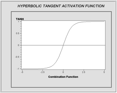
In SAS Enterprise Miner, a variety of activation functions are available for use in the hidden layers. These include Arc Tangent, Elliot, Hyperbolic Tangent, Logistic, Gauss, Sine, and Cosine, in addition to several other types of activation functions discussed in Section 5.7.

The four activation functions, Arc Tangent, Elliot, Hyperbolic Tangent and Logistic, are called Sigmoid functions; they are S-shaped and give values that are bounded within the range of 0 to 1 or –1 to 1.

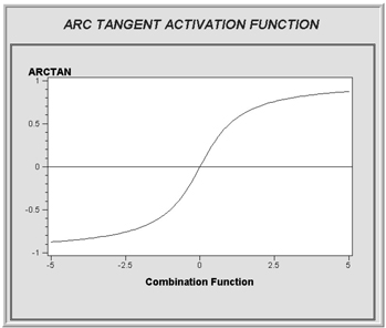
The hyperbolic tangent function shown in Display 5.0B has values bounded between –1 and 1. Displays 5.0C, 5.0D, and 5.0E show Logistic, Arc Tangent, and Elliot functions, respectively.

Display 5.0C

Display 5.0D

Display 5.0E

In general, wmkj $w_{m k j}$ is the weight of the mth $m^{t h}$ input in the jth $j^{t h}$ neuron (unit) of the kth $k^{t h}$ hidden layer, and w0kj $w_{0 k j}$ is the corresponding bias. The weighted sum and the output calculated by the jth $j^{t h}$ neuron in the kth $k^{t h}$ hidden layer are ηikj $η_{i k j}$ and Hikj $H_{i k j}$ , respectively, where i $i$ stands for the ith $i^{t h}$ record in the data set.

Hidden Layer 1: Unit 2

The calculation of the output of unit 2 proceeds in the same way as in unit 1, but with a different set of weights and bias. The weighted sum of the inputs for the ith $i^{t h}$ person or record in the data is

η i 12 = w 012 + w 112 x i 1 + w 212 x i 2 + ... w p 12 x i p . (5.3)

$η_{i 12} = w_{012} + w_{112} x_{i 1} + w_{212} x_{i 2} + ... w_{p 12} x_{i p} . (5.3)$

The output of unit 2 is:

H i 12 = tanh (η i 12) = exp ( η i 12 ) - exp ( - η i 12 ) exp ( η i 12 ) + exp ( - η i 12 ) (5.4)

$H_{i 12} = \tanh (η_{i 12}) = \frac{\exp (η_{i 12}) - \exp (- η_{i 12})}{\exp (η_{i 12}) + \exp (- η_{i 12})} (5.4)$

Hidden Layer 1: Unit 3

The calculations in unit 3 proceed exactly as in units 1 and 2, but with a different set of weights and bias. The weighted sum of the inputs for ith $i^{t h}$ person in the data set is

η i 13 = w 013 + w 113 x i 1 + w 213 x i 2 + ... w p 13 x i p, (5.5)

$η_{i 13} = w_{013} + w_{113} x_{i 1} + w_{213} x_{i 2} + ... w_{p 13} x_{i p}, (5.5)$

and the output of this unit is:

H i 13 = tanh (η i 13) = exp ( η i 13 ) - exp ( - η i 13 ) exp ( η i 13 ) + exp ( - η i 13 ) (5.6)

$H_{i 13} = \tanh (η_{i 13}) = \frac{\exp (η_{i 13}) - \exp (- η_{i 13})}{\exp (η_{i 13}) + \exp (- η_{i 13})} (5.6)$

5.2.2.2 Hidden Layer 2

There are three units in this layer, each producing an intermediate output based on the inputs it receives from the previous layer.

Hidden Layer 2: Unit 1

The weighted sum of the inputs calculated by this unit is:

η i 21 = w 021 + w 121 H i 11 + w 221 H i 12 + w 321 H i 13 (5.7)

$η_{i 21} = w_{021} + w_{121} H_{i 11} + w_{221} H_{i 12} + w_{321} H_{i 13} (5.7)$

ηi21 $η_{i 21}$ is the weighted sum for the ith $i^{t h}$ record in the data set in unit 1 of layer 2.

The output of this unit is:

H i 21 = tanh (η i 21) = exp ( η i 21 ) - exp ( - η i 21 ) exp ( η i 21 ) + exp ( - η i 21 ) (5.8)

$H_{i 21} = \tanh (η_{i 21}) = \frac{\exp (η_{i 21}) - \exp (- η_{i 21})}{\exp (η_{i 21}) + \exp (- η_{i 21})} (5.8)$

Hidden Layer 2: Unit 2

The weighted sum of the inputs for the ith $i^{t h}$ person or record in the data is

η i 22 = w 022 + w 122 H i 11 + w 222 H i 12 + w 322 H i 13, (5.9)

$η_{i 22} = w_{022} + w_{122} H_{i 11} + w_{222} H_{i 12} + w_{322} H_{i 13}, (5.9)$

and the output of this unit is:

H i 22 = tanh (η i 22) = exp ( η i 22 ) - exp ( - η i 22 ) exp ( η i 22 ) + exp ( - η i 22 ) (5.10)

$H_{i 22} = \tanh (η_{i 22}) = \frac{\exp (η_{i 22}) - \exp (- η_{i 22})}{\exp (η_{i 22}) + \exp (- η_{i 22})} (5.10)$

Hidden Layer 2: Unit 3

The weighted sum of the inputs for ith $i^{t h}$ person in the data set is

η i 23 = w 023 + w 123 H i 11 + w 223 H i 12 + w 323 H i 13, (5.11)

$η_{i 23} = w_{023} + w_{123} H_{i 11} + w_{223} H_{i 12} + w_{323} H_{i 13}, (5.11)$

and the output of this unit is:

H i 23 = tanh (η i 23) = exp ( η i 23 ) - exp ( - η i 23 ) exp ( η i 23 ) + exp ( - η i 23 ) (5.12)

$H_{i 23} = \tanh (η_{i 23}) = \frac{\exp (η_{i 23}) - \exp (- η_{i 23})}{\exp (η_{i 23}) + \exp (- η_{i 23})} (5.12)$

5.2.3 Output Layer or Target Layer

This layer produces the final output of the neural network—the predicted values of the targets. In the case of a response model, the output of this layer is the predicted probability of response and non-response, and the output layer has two units. In the case of a categorical target with more than two levels, there are more than two output units. When the target is continuous, such as a bank account balance, the output is the expected value. Display 5.0A shows k outputs, and they are: y1,y2,.......,yk $y_{1}, y_{2}, ......., y_{k}$ . For the response model k=2, and for the loss frequency (risk) model k=3.

The inputs into this layer are Hi21, Hi22, and Hi23 $H_{i 21}, H_{i 22}, and H_{i 23}$ , which are the intermediate outputs produced by the preceding layer. These intermediate outputs can be thought of as the nonlinear transformations and combinations of the original inputs performed through successive layers of the network, as described in Equations 5.1 through 5.13. Hi21, Hi22, and Hi23 $H_{i 21}, H_{i 22}, and H_{i 23}$ can be considered synthetic variables constructed from the inputs.

In the output layer, these transformed inputs (Hi21, Hi22, and Hi23 $H_{i 21}, H_{i 22}, and H_{i 23}$ ) are used to construct predictive equations of the target. First, for each output unit, a linear combination of Hi21, Hi22, and Hi23 $H_{i 21}, H_{i 22}, and H_{i 23}$ , called a linear predictor (or combination function), is defined and an activation function is specified to give the desired predictive equation.

In the case of response model, the first output unit gives the probability of response represented by y1 $y_{1}$ , while the second output unit gives the probability of no response represented by y2 $y_{2}$ . In the case of the loss frequency model, there are three outputs: y1,y2,and y3 $y_{1}, y_{2}, and y_{3}$ . The first output unit gives the probability that LOSSFRQ is 0 (y1 $y_{1}$ ), the second output unit gives the probability that LOSSFRQ is 1 (y2 $y_{2}$ ), and the third output gives the probability that LOSSFRQ is (y3 $y_{3}$ ).

The linear combination of the inputs from the previous layer is calculated as:

η i 31 = w 031 + w 131 H i 21 + w 231 H i 22 + w 331 H i 23 (5.13)

$η_{i 31} = w_{031} + w_{131} H_{i 21} + w_{231} H_{i 22} + w_{331} H_{i 23} (5.13)$

Equation 5.13 is the linear predictor (or linear combination function), because it is linear in terms of the weights.

5.2.4 Activation Function of the Output Layer

The activation function is a formula for calculating the target values from the inputs coming from the final hidden layer. The outputs of the final hidden layer are first combined as shown in Equation 5.13. The resulting combination is transformed using the activation function to give the final target values. The activation function is chosen according to the type of target and what you are interested in predicting. In the case of a binary target I use a logistic activation function in the final output or target layer wherein the ith $i^{t h}$ person’s probability of response (πi $π_{i}$ ) is calculated as:

π i = exp ( η i 31 ) 1 + exp ( η i 31 ) = 1 1 + exp ( - η i 31 ) (5.14)

$π_{i} = \frac{\exp (η_{i 31})}{1 + \exp (η_{i 31})} = \frac{1}{1 + \exp (- η_{i 31})} (5.14)$

Equation 5.14 is called the logistic activation function, and is based on a logistic distribution. By substituting Equations 5.1 through 5.13 into Equation 5.14, I can easily verify that it is possible to write the output of this node as an explicit nonlinear function of the weights and the inputs. This can be denoted by:

π i (W, X i) (5.15)

$π_{i} (W, X_{i}) (5.15)$

In Equation 5.15, W $W$ is the vector whose elements are the weights shown in Equations 5.1, 5.3, 5.5, 5.7, 5.9, 5.11, and 5.13, and Xi $X_{i}$ is the vector of inputs xi1, xi2, . . . xip $x_{i 1}, x_{i 2}, . . . x_{i p}$ for the ith $i^{t h}$ person in the data set.

The neural network described above is called a multilayer perceptron or MLP. In general, a network that uses linear combination functions and sigmoid activation functions in the hidden layers is called a multilayer perceptron. In SAS Enterprise Miner, if you set the Architecture property to MLP, then you get an MLP with only one hidden layer.

5.3 Estimation of Weights in a Neural Network Model

The weights are estimated iteratively using the training data set in such a way that the error function specified by the user is minimized. In the case of a response model, I use the following Bernoulli error function:

E = - 2 \sum i = 1 n {y i ln π ( W , X i ) y i + (1 - y i) ln 1 - π ( W , X i ) 1 - y i} (5.16)

$E = - 2 \sum_{i = 1}^{n} {y_{i} \ln \frac{π (W, X_{i})}{y_{i}} + (1 - y_{i}) \ln \frac{1 - π (W, X_{i})}{1 - y_{i}}} (5.16)$

where π $π$ is the estimated probability of response. It is a function of the vector of weights, W $W$ , and the vector of explanatory variables for the ith $i^{t h}$ person, Xi $X_{i}$ . The variable yi $y_{i}$ is the observed response of the ith $i^{t h}$ person, in which yi=1 $y_{i} = 1$ if the ith $i^{t h}$ person responded to direct mail and yi=0 $y_{i} = 0$ if the ith $i^{t h}$ person did not respond. If yi $y_{i}$ =1 for the ith $i^{t h}$ observation, then its contribution to the error function (Equation 5.16) is −2logπ(W,Xi) $- 2 \log π (W, X_{i})$ ; if yi=0 $y_{i} = 0$ , then the contribution is −2log(1−π(W,Xi)) $- 2 \log (1 - π (W, X_{i}))$ .

The total number of observations in the Training data set is n $n$ . The error function is summed over all of these observations. The inputs for the ith $i^{t h}$ record are known, and the values for the weights W $W$ are chosen so as to minimize the error function. A number of iterative methods of finding the optimum weights are discussed in Bishop.³

In general, the calculation of the optimum weights is done in two steps:

Step 1: Finding the error-minimizing weights from the Training data set

In the first step, an iterative procedure is used with the training data set to find a set of weights that minimize the error function given in Equation 5.16. In the first iteration, a set of initial weights is used, and the error function Equation 5.16 is evaluated. In the second iteration, the weights are changed by a small amount in such a way that the error is reduced. This process continues until the error cannot be further reduced, or until the specified maximum number of iterations is reached. At each iteration, a set of weights is generated. If it takes 100 iterations to find the error-minimizing weights for the Training data set, then 100 sets of weights are generated and saved. Thus, the training process generates 100 models in this example. The next task is to select the best model out of these 100 models. This is done using the Validation data set.

Step 2: Finding the optimum weights from the Validation data set.

In this step, the user-supplied Model Selection Criterion is applied to select one of the 100 sets of weights generated in step 1. This selection is done using the Validation data set. Suppose I set the Model Selection Criterion property to Average Error. Then the average error is calculated for each of the 100 models using the Validation data set. If the Validation data set has m observations, then the error calculated from the weights generated at the kth $k_{t h}$ iteration is

E (k) = - 2 \sum i = 1 m {y i ln π ( W ( k ) , X i ) y i + (1 - y i) ln 1 - π ( W ( k ) , X i ) 1 - y i} (5.17)

$E_{(k)} = - 2 \sum_{i = 1}^{m} {y_{i} \ln \frac{π (W_{(k)}, X_{i})}{y_{i}} + (1 - y_{i}) \ln \frac{1 - π (W_{(k)}, X_{i})}{1 - y_{i}}} (5.17)$

where yi=1 $y_{i} = 1$ for a responder, and 0 for a non-responder. The average error at the kth $k_{t h}$ iteration is E(k)2m $\frac{E_{(k)}}{2 m}$ . The set of weights with the smallest average error is used in the final predictive equation. Alternative model selection criteria can be chosen by changing the Model Selection Criterion property.

As pointed out earlier, Equations 5.1, 5.3, 5.5, 5.7, 5.9, 5.11, and 5.13 are called combination functions, and Equations 5.2, 5.4, 5.6, 5.8, 5.10, 5.12, and 5.14 are called activation functions.

By substituting Equations 5.1 through 5.13 into Equation 5.14, I can write the neural network model as an explicit function of the inputs. This is an arbitrary nonlinear function, and its complexity (and hence the degree of nonlinearity) depends on network features such as the number of hidden layers included, the number of units in each hidden layer, and the combination and activation functions in each hidden unit.

In the neural network model described above, the final layer inputs (Hi21,Hi22, and Hi23 $H_{i 21}, H_{i 22}, and H_{i 23}$ ) can be thought of as final transformations of the original inputs made by the calculations in different layers of the network.

In each hidden unit, I used a linear combination function to calculate the weighted sum of the inputs, and a hyperbolic tangent activation function to calculate the intermediate output for each hidden unit. In the output layer, I specified a linear combination function and a logistic activation function. The error function I specified is called the Bernoulli error function. A neural network with two hidden layers and one output layer is called a three-layered network. In characterizing the network, the input layer is not counted, since units in the input layer do not perform any computations except standardizing the inputs.

5.4 A Neural Network Model to Predict Response

This section discusses the neural network model developed to predict the response to a planned direct mail campaign. The campaign’s purpose is to solicit customers for a hypothetical insurance company. A two-layered network with one hidden layer was chosen. Three units are included in the hidden layer. In the hidden layer, the combination function chosen is linear, and the activation function is hyperbolic tangent. In the output layer, a logistic activation function and Bernoulli error function are used. The logistic activation function results in a logistic regression type model with non-linear transformation of the inputs, as shown in Equation 5.14 in Section 5.2.4. Models of this type are in general estimated by minimizing the Bernoulli error functions shown in Equation 5.16. Minimization of the Bernoulli error function is equivalent to maximizing the likelihood function.

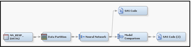
Display 5.1 shows the process flow for the response model. The first node in the process flow diagram is the Input Data node, which makes the SAS data set available for modeling. The next node is Data Partition, which creates the Training, Validation, and Test data sets. The Training data set is used for preliminary model fitting. The Validation data set is used for selecting the optimum weights. The Model Selection Criterion property is set to Average Error.

As pointed out earlier, the estimation of the weights is done by minimizing the error function. This minimization is done by an iterative procedure. Each iteration yields a set of weights. Each set of weights defines a model. If I set the Model Selection Criterion property to Average Error, the algorithm selects the set of weights that results in the smallest error, where the error is calculated from the Validation data set.

Since both the Training and Validation data sets are used for parameter estimation and parameter selection, respectively, an additional holdout data set is required for an independent assessment of the model. The Test data set is set aside for this purpose.

Display 5.1

Input Data Node

I create the data source for the Input Data node from the data set NN_RESP_DATA2. I create the metadata using the Advanced Advisor Options, and I customize it by setting the Class Levels Count Threshold property to 8, as shown in Display 5.2

Display 5.2

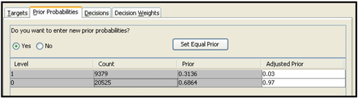
I set adjusted prior probabilities to 0.03 for response and 0.97 for non-response, as shown in Display 5.3.

Display 5.3

Data Partition Node

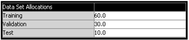
The input data is partitioned such that 60% of the observations are allocated for training, 30% for validation, and 10% for Test, as shown in Display 5.4.

Display 5.4

5.4.1 Setting the Neural Network Node Properties

Here is a summary of the neural network specifications for this application:

• One hidden layer with three neurons

• Linear combination functions for both the hidden and output layers

• Hyperbolic tangent activation functions for the hidden units

• Logistic activation functions for the output units

• The Bernoulli error function

• The Model Selection Criterion is Average Error

These settings are shown in Displays 5.5–5.7.

Display 5.5 shows the Properties panel for the Neural Network node.

Display 5.5

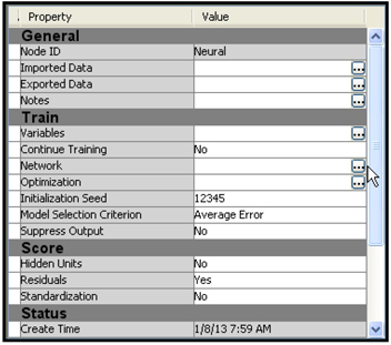
To define the network architecture, click located to the right of the Network property. The Network Properties panel opens, as shown in Display 5.6.

Display 5.6

Set the properties as shown in Display 5.6 and click OK.

To set the iteration limit, click located to the right of the Optimization property. The Optimization Properties panel opens, as shown in Display 5.7. Set Maximum Iterations to 100.

Display 5.7

After running the Neural Network node, you can open the Results window, shown in Display 5.8. The window contains four windows: Score Rankings Overlay, Iteration Plot, Fit Statistics, and Output.

Display 5.8

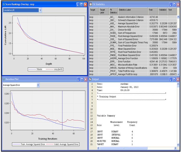
The Score Rankings Overlay window in Display 5.8 shows the cumulative lift for the Training and Validation data sets. Click the down arrow next to the text box to see a list of available charts that can be displayed in this window.

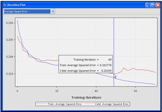
Display 5.9 shows the iteration plot with Average Squared Error at each iteration for the Training and Validation data sets. The estimation process required 70 iterations. The weights from the 49^th iteration were selected. After the 49^th iteration, the Average Squared Error started to increase in the Validation data set, although it continued to decline in the Training data set.

Display 5.9

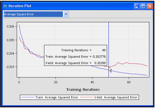
You can save the table corresponding to the plot shown in Display 5.9 by clicking the Tables icon and then selecting File→ Save As. Table 5.1 shows the three variables _ITER_ (iteration number), _ASE_ (Average Squared Error for the Training data), and _VASE_ (Average Squared Error from the Validation data) at iterations 41-60.

Table 5.1

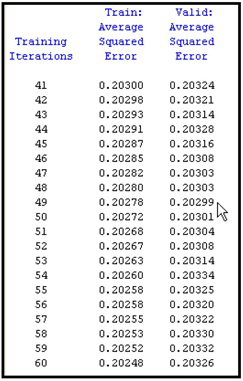
You can print the variables _ITER_, _ASE_, and _VASE_ by using the SAS code shown in Display 5.10.

Display 5.10

5.4.2 Assessing the Predictive Performance of the Estimated Model

In order to assess the predictive performance of the neural network model, run the Model Comparison node and open the Results window. In the Results window, the Score Rankings Overlay shows the Lift charts for the Training, Validation, and Test data sets. These are shown in Display 5.11.

Display 5.11

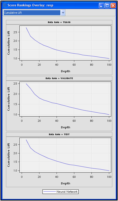
Click the arrow in the box at the top left corner of the Score Ranking Overlay window to see a list of available charts.

SAS Enterprise Miner saves the Score Rankings table as EMWS.MdlComp_EMRANK. Tables 5.2, 5.3, and 5.4 are created from the saved data set using the simple SAS code shown in Display 5.12.

Display 5.12

Table 5.2

Table 5.3

Table 5.4

The lift and capture rates calculated from the Test data set (shown in Table 5.4) should be used for evaluating the models or comparing the models because the Test data set is not used in training or fine-tuning the model.

To calculate the lift and capture rates, SAS Enterprise Miner first calculates the predicted probability of response for each record in the Test data. Then it sorts the records in descending order of the predicted probabilities (also called the scores) and divides the data set into 20 groups of equal size. In Table 5.4, the column Bin shows the ranking of these groups. If the model is accurate, the table should show the highest actual response rate in the first bin, the second highest in the next bin, and so on. From the column %Response, it is clear that the average response rate for observations in the first bin is 8.36796%. The average response rate for the entire test data set is 3%. Hence the lift for Bin 1, which is the ratio of the response rate in Bin 1 to the overall response rate, is 2.7893. The lift for each bin is calculated in the same way. The first row of the column Cumulative %Response shows the response rate for the first bin. The second row shows the response rate for bins 1 and 2 combined, and so on.

The capture rate of a bin shows the percentage of likely responders that it is reasonable to expect to be captured in the bin. From the column Captured Response, you can see that 13.951% of all responders are in Bin 1.

From the Cumulative % Captured Response column of Table 5.3, you can be seen that, by sending mail to customers in the first four bins, or the top 20% of the target population, it is reasonable to expect to capture 39% of all potential responders from the target population. This assumes that the modeling sample represents the target population.

5.4.3 Receiver Operating Characteristic (ROC) Charts

Display 5.13, taken from the Results window of the Model Comparison node, displays ROC curves for the Training, Validation, and Test data sets. An ROC curve shows the values of the true positive fraction and the false positive fraction at different cut-off values, which can be denoted by Pc $P_{c}$ . In the case of the response model, if the estimated probability of response for a customer record were above a cut-off value Pc $P_{c}$ , then you would classify the customer as a responder; otherwise, you would classify the customer as a non-responder.

Display 5.13

In the ROC chart, the true positive fraction is shown on the vertical axis, and the false positive fraction is on the horizontal axis for each cut-off value (Pc $P_{c}$ ).

If the calculated probability of response (P_resp1) is greater than equal to the cut-off value, then the customer (observation) is classified as a responder. Otherwise, the customer is classified as non-responder.

True positive fraction is the proportion of responders correctly classified as responders. The false positive fraction is the proportion of non-responders incorrectly classified as responders. The true positive fraction is also called sensitivity, and specificity is the proportion of non-responders correctly classified as non-responders. Hence, the false positive fraction is 1-specificity. An ROC curve reflects the tradeoff between sensitivity and specificity.

The straight diagonal lines in Display 5.13 that are labeled Baseline are the ROC charts of a model that assigns customers at random to the responder group and the non-responder group, and hence has no predictive power. On these lines, sensitivity = 1- specificity at all cut-off points. The larger the area between the ROC curve of the model being evaluated and the diagonal line, the better the model. The area under the ROC curve is a measure of the predictive accuracy of the model and can be used for comparing different models.

Table 5.5 shows sensitivity and 1-specificity at various cut-off points in the validation data.

Table 5.5

From Table 5.5, you can see that at a cut-off probability (Pc $P_{c}$ ) of 0.02, for example, the sensitivity is 0.84115. That is, at this cut-off point, you will correctly classify 84.1% of responders as responders, but you will also incorrectly classify 68.1% of non-responders as responders, since 1-specificity at this point is 0.68139. If instead you chose a much higher cut-off point of Pc $P_{c}$ = 0.13954, you would classify 0.284% of true responders as responders and 0.049% of non-responders as responders. In this case, by increasing the cut-off probability beyond which you would classify an individual as a responder, you would be reducing the fraction of false positive decisions made, while, at the same time, also reducing the fraction of true positive decisions made. These pairings of a true positive fraction with a false positive fraction are plotted as the ROC curve for the VALIDATE case in Display 5.13.

The SAS macro in Display 5.14 demonstrates the calculation of the true positive rate (TPR) and the false positive rate (FPR) at the cut-off probability of 0.02.

Display 5.14

Tables 5.6, 5.7, and 5.8, generated by the macro shown in Display 5.14, show the sequence of steps for calculating TPR and FPR for a given cut-off probability.

Table 5.6

Table 5.7

Table 5.8

For more information about ROC curves, see the textbook by A. A. Afifi and Virginia Clark (2004).⁴

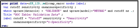
Display 5.15 shows the SAS code that generated Table 5.5.

Display 5.15

5.4.4 How Did the Neural Network Node Pick the Optimum Weights for This Model?

In Section 5.3, I described how the optimum weights are found in a neural network model. I described the two-step procedure of estimating and selecting the weights. In this section, I show the results of these two steps with reference to the neural network model discussed in Sections 5.4.1 and 5.4.2.

The weights such as those shown in Equations 5.1, 5.3, 5.5, 5.7, 5.9, 5.11, and 5.13 are shown in the Results window of the Neural Network node. You can see the estimated weights created at each iteration by opening the results window and selecting View→Model→Weights-History. Display 5.16 shows a partial view of the Weights-History window.

Display 5.16

The second column in Display 5.16 shows the weight of the variable AGE in hidden unit 1 at each iteration. The seventh column shows the weight of AGE in hidden unit 2 at each iteration. The twelfth column shows the weight of AGE in the third hidden unit. Similarly, you can trace through the weights of other variables. You can save the Weights-History table as a SAS data set.

To see the final weights, open the Results window. Select View→Model→Weights_Final. Then, click the Table icon. Selected rows of the final weights_table are shown in Display 5.17.

Display 5.17

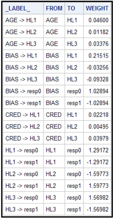
Outputs of the hidden units become inputs to the target layer. In the target layer, these inputs are combined using the weights estimated by the Neural Network node.

In the model I have developed, the weights generated at the 49^th iteration are the optimal weights, because the Average Squared Error computed from the Validation data set reaches its minimum at the 49^th iteration. This is shown in Display 5.18.

Display 5.18

5.4.5 Scoring a Data Set Using the Neural Network Model

You can use the SAS code generated by the Neural Network node to score a data set within SAS Enterprise Miner or outside. This example scores a data set inside SAS Enterprise Miner.

The process flow diagram with a scoring data set is shown in Display 5.19.

Display 5.19

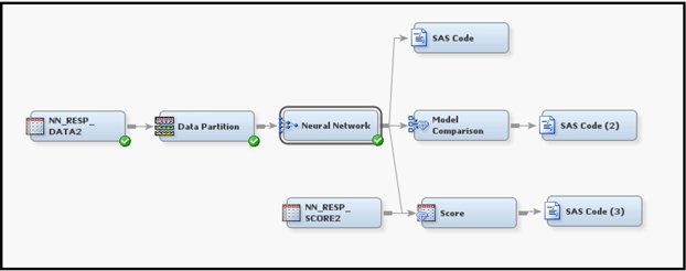
Set the Role property of the data set to be scored to Score, as shown in Display 5.20.

Display 5.20

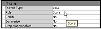
The Score Node applies the SAS code generated by the Neural Network node to the Score data set NN_RESP_SCORE2, shown in Display 5.19.

For each record, the probability of response, the probability of non-response, and the expected profit of each record is calculated and appended to the scored data set.

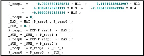
Display 5.21 shows the segment of the score code where the probabilities of response and non-response are calculated. The coefficients of HL1, HL2, and HL3 in Display 5.21 are the weights in the final output layer. These are same as the coefficients shown in Display 5.17.

Display 5.21

The code segment given in Display 5.21 calculates the probability of response using the formula P_resp1i=11+exp(−ηi21) $P_r e s p 1_{i} = \frac{1}{1 + \exp (- η_{i 21})}$ ,

where μi21 $μ_{i 21}$ = -1.29172481842873 * HL1 + 1.59773122184585 * HL2

+ -1.56981973539319 * HL3 -1.0289412689995;

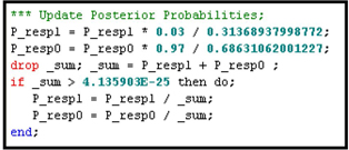
This formula is the same as Equation 5.14 in Section 5.2.4. The subscript i $i$ is added to emphasize that this is a record-level calculation. In the code shown in Display 5.21, the probability of non-response is calculated as p_resp0=11+exp(ηi21) $p_r e s p 0 = \frac{1}{1 + \exp (η_{i 21})}$ .

The probabilities calculated above are modified by the prior probabilities I entered prior to running the Neural Network node. These probabilities are shown in Display 5.22.

Display 5.22

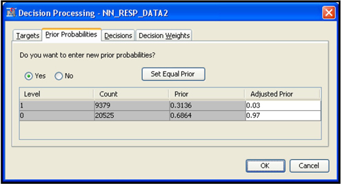
You can enter the prior probabilities when you create the Data Source. Prior probabilities are entered because the responders are overrepresented in the modeling sample, which is extracted from a larger sample. In the larger sample, the proportion of responders is only 3%. In the modeling sample, the proportion of responders is 31.36%. Hence, the probabilities should be adjusted before expected profits are computed. The SAS code generated by the Neural Network node and passed on to the Score node includes statements for making this adjustment. Display 5.23 shows these statements.

Display 5.23

Display 5.24 shows the profit matrix used in the decision-making process.

Display 5.24

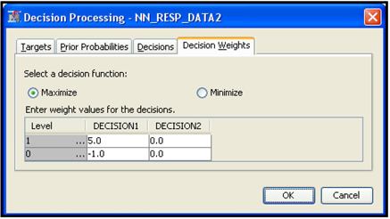
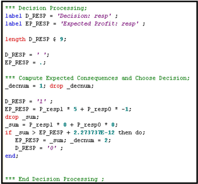
Given the above profit matrix, calculation of expected profit under the alternative decisions of classifying an individual as responder or non-responder proceeds as follows. Using the neural network model, the scoring algorithm first calculates the individual’s probability of response and non-response. Suppose the calculated probability of response for an individual is 0.3, and probability of non-response is 0.7. The expected profit if the individual is classified as responder is 0.3x$5 + 0.7x (–$1.0) = $0.8. The expected profit if the individual is classified as non-responder is 0.3x ($0) + 0.7x ($0) = $0. Hence classifying the individual as responder (Decision1) yields a higher profit than if the individual is classified as non-responder (Decision2). An additional field is added to the record in the scored data set indicating the decision to classify the individual as a responder.

These calculations are shown in the score code segment shown in Display 5.25.

Display 5.25

5.4.6 Score Code

The score code is automatically saved by the Score node in the sub-directory WorkspacesEMWSnScore within the project directory.

For example, in my computer, the Score code is saved by the Score node in the folder C:TheBookEM12.1EMProjectsChapter5WorkspacesEMWS3Score. Alternatively, you can save the score code in some other directory. To do so, run the Score node, and then click Results. Select either the Optimized SAS Code window or the SAS Code window. Click File→Save As, and enter the directory and name for saving the score code.

5.5 A Neural Network Model to Predict Loss Frequency in Auto Insurance

The premium that an insurance company charges a customer is based on the degree of risk of monetary loss to which the customer exposes the insurance company. The higher the risk, the higher the premium the company charges. For proper rate setting, it is essential to predict the degree of risk associated with each current or prospective customer. Neural networks can be used to develop models to predict the risk associated with each individual.

In this example, I develop a neural network model to predict loss frequency at the customer level. I use the target variable LOSSFRQ that is a discrete version of loss frequency. The definition of LOSSFRQ is presented in the beginning of this chapter (Section 5.1.1). If the target is a discrete form of a continuous variable with more than two levels, it should be treated as an ordinal variable, as I do in this example.

I have already discussed the general framework for neural network models in Section 5.2. There I gave an example of a neural network model with two hidden layers. I also pointed out that the outputs of the final hidden layer can be considered as complex transformations of the original inputs. These are given in Equations 5.1 through 5.12.

In the following example, there is only one hidden layer, and it has three units. The outputs of the hidden layer are HL1 $H_{L 1}$ , HL2 $H_{L 2}$ , and HL3 $H_{L 3}$ . Since these are nothing but transformations of the original inputs, I can write the desired conditional probabilities as
Pr(LOSSFRQ=0|HL1,HL2,and HL3) $\Pr (L O S S F R Q = 0 | H_{L 1}, H_{L 2}, a n d H_{L 3})$ , Pr(LOSSFRQ=1|HL1,HL2,and HL3) $\Pr (L O S S F R Q = 1 | H_{L 1}, H_{L 2}, a n d H_{L 3})$ ,
and Pr(LOSSFRQ=2|HL1,HL2,and HL3) $\Pr (L O S S F R Q = 2 | H_{L 1}, H_{L 2}, a n d H_{L 3})$ .

5.5.1 Loss Frequency as an Ordinal Target

In order for the Neural Network node to treat the target variable LOSSFRQ as an ordinal variable, we should set its measurement level to Ordinal in the data source.

Display 5.26 shows the process flow diagram for developing a neural network model.

Display 5.26

The data source for the Input Data node is created from the data set Ch5_LOSSDAT2 using the Advanced Metadata Advisor Options with the Class Levels Count Threshold property set to 8, which is the same setting shown in Display 5.2.

As pointed out in Section 5.1.1, loss frequency is a continuous variable. The target variable LOSSFRQ, used in the Neural Network model developed here, is a discrete version of loss frequency. It is created as follows:

L O S S F R Q = 0 i f l o s s f r e q u e n c y = 0, L O S S F R Q = 1 i f 0 < l o s s f r e q u e n c y < 1.5, a n d L O S S F R Q = 2 i f l o s s f r e q u e n c y \geq 1.5.

Display 5.27 shows a partial list of the variables contained in the data set Ch5_LOSSDAT2. The target variable is LOSSFRQ. I changed its measurement level from Nominal to Ordinal.

Display 5.27

For illustration purposes, I enter a profit matrix, which is shown in Display 5.28. A profit matrix can be used for classifying customers into different risk groups such as low, medium, and high.

Display 5.28

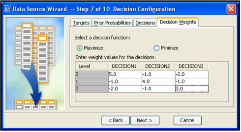
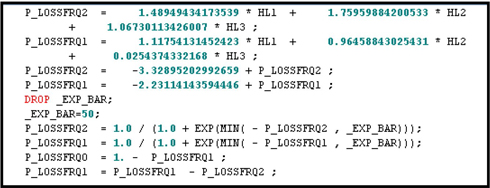
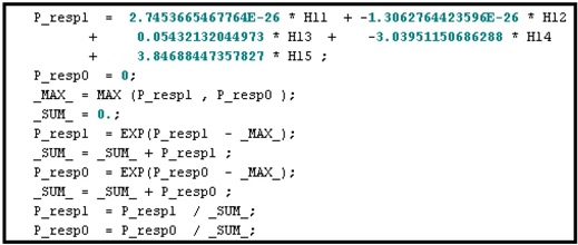
The SAS code generated by the Neural Network node, shown in Display 5.29, illustrates how the profit matrix shown in Display 5.28 is used to classify customers into different risk groups.

Display 5.29

In the SAS code shown in Display 5.29, P_LOSSFRQ2, P_LOSSFRQ1, and P_LOSSFRQ0 are the estimated probabilities of LOSSFRQ= 2, 1, and 0, respectively, for each customer.

The property settings of the Data Partition node for allocating records for Training, Validation, and Test are 60, 30, and 10, respectively. These settings are the same as in Display 5.4.

To define the Neural Network, click located to the right of the Network property of the Neural Network node. The Network window opens, as shown in Display 30.

Display 5.30

The general formulas of Combination Functions and Activation Functions of the hidden layers are given by equations 5.1-5.12 of section 5.2.2.

In the Neural Network model developed in this section, there is only one hidden layer and three hidden units, each hidden unit producing an output. The outputs produced by the hidden units are HL1, HL2, and HL3. These are special variables that are constructed from inputs contained in the dataset Ch5_LOSSDAT2. These inputs are standardized prior to being used by the hidden layer.

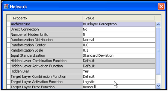
5.5.1.1 Target Layer Combination and Activation Functions

As you can see from Display 5.30, I set the Target Layer Combination Function property to Linear and the Target Layer Activation Function property to Logistic. These settings result in the following calculations.

Since we set the Target Layer Combination Function property to be linear, the Neural Network node calculates linear predictors for each observation from the hidden layer outputs HL1, HL2, and HL3. Since the target variable LOSSFRQ is ordinal, taking the values 0, 1 and 2, the Neural Network node calculates two linear predictors.

The first linear predictor for the ith $i^{t h}$ customer/record is calculated as:

μi1=w10+w11HL1i+w12HL2i+w13HL3i $μ_{i 1} = w_{10} + w_{11} H L 1_{i} + w_{12} H L 2_{i} + w_{13} H L 3_{i}$ (5.18)

μi1 $μ_{i 1}$ is the linear predictor used in the calculation of P(LOSSFRQ=2/Hi) $P (L O S S F R Q = 2 / H_{i})$ for the ith $i^{t h}$ customer/record.

where Hi=⎛⎝⎜⎜⎜1HL1iHL2iHL3i⎞⎠⎟⎟⎟ $w h e r e H_{i} = (\begin{array}{l} 1 \\ H L 1_{i} \\ H L 2_{i} \\ H L 3_{i} \end{array})$ ,

HL1i=Output of the first hidden unit for the ith customer, HL2i=Output of the second hidden unit for the ith customer,HL3i=Output of the third hidden unit for the ith customer, $\begin{array}{l} H L 1_{i} = {Output of the first hidden unit for the i}^{t h} customer, \\ H L 2_{i} = {Output of the second hidden unit for the i}^{t h} customer, \\ H L 3_{i} = {Output of the third hidden unit for the i}^{t h} customer, \end{array}$

w11,w12 and w13 $w_{11}, w_{12} and w_{13}$ are the weights of the outputs of the hidden units, and w10 $w_{10}$ is the bias.

The estimated values of the bias and weights are:

w10=−3.328952w11=1.489494w12=1.759599w13=1.067301 $\begin{array}{l} w_{10} = - 3.328952 \\ w_{11} = 1.489494 \\ w_{12} = 1.759599 \\ w_{13} = 1.067301 \end{array}$

The second linear predictor for the ith $i^{t h}$ customer/record is calculated as:

μi2=w20+w21HL1i+w22HL2i+w23HL3i $μ_{i 2} = w_{20} + w_{21} H L 1_{i} + w_{22} H L 2_{i} + w_{23} H L 3_{i}$ (5.19)

The estimated values of the bias and weights are:

w20=−2.23114w21=1.11754w22=0.96459w23=0.02544 $\begin{array}{l} w_{20} = - 2.23114 \\ w_{21} = 1.11754 \\ w_{22} = 0.96459 \\ w_{23} = 0.02544 \end{array}$

μi2 $μ_{i 2}$ is the linear predictor used in the calculation of P(LOSSFRQ=2/Hi)+P(LOSSFRQ=1/Hi) $P (L O S S F R Q = 2 / H_{i}) + P (L O S S F R Q = 1 / H_{i})$ for the ith $i^{t h}$ customer/record.

μi1 $μ_{i 1}$ and μi2 $μ_{i 2}$ are treated as logits. That is,

μi1=log[P(LOSSFRQ=2|Hi)1−P(LOSSFRQ=2|Hi)] $μ_{i 1} = \log [\frac{P (L O S S F R Q = 2 | H_{i})}{1 - P (L O S S F R Q = 2 | H_{i})}]$ (5.20)

μi2=log[P(LOSSFRQ=2|Hi)+P(LOSSFRQ=1|Hi)1−{P(LOSSFRQ=2|Hi)+P(LOSSFRQ=1|Hi)}] $μ_{i 2} = \log [\frac{P (L O S S F R Q = 2 | H_{i}) + P (L O S S F R Q = 1 | H_{i})}{1 - {P (L O S S F R Q = 2 | H_{i}) + P (L O S S F R Q = 1 | H_{i})}}]$ (5.21)

Since μi1 $μ_{i 1}$ is based on P(LOSSFRQ=2|Hi) $P (L O S S F R Q = 2 | H_{i})$ and μi2 $μ_{i 2}$ is based on P(LOSSFRQ=2|Hi)+P(LOSSFRQ=1|Hi) $P (L O S S F R Q = 2 | H_{i}) + P (L O S S F R Q = 1 | H_{i})$ , μi1 $μ_{i 1}$ and μi2 $μ_{i 2}$ can be called cumulative logits, and the model estimated by this procedure can be called a Cumulative Logits model. Given μi1 $μ_{i 1}$ and μi2 $μ_{i 2}$ , we can calculate the probabilities P(LOSSFRQ=2|Hi), $P (L O S S F R Q = 2 | H_{i}),$ P(LOSSFRQ=1|Hi) $P (L O S S F R Q = 1 | H_{i})$ and P(LOSSFRQ=0|Hi) $P (L O S S F R Q = 0 | H_{i})$ in the following way:

P(LOSSFRQ=2∣∣Hi)=11+exp(−μi1) $P (L O S S F R Q = 2 | H_{i}) = \frac{1}{1 + \exp (- μ_{i 1})}$ (5.22)

P(LOSSFRQ=2∣∣Hi)+P(LOSSFRQ=1∣∣Hi)=11+exp(−μi2) $P (L O S S F R Q = 2 | H_{i}) + P (L O S S F R Q = 1 | H_{i}) = \frac{1}{1 + \exp (- μ_{i 2})}$ (5.23)

P(LOSSFRQ=0|Hi)=1−[P(LOSSFRQ=2|Hi)+P(LOSSFRQ=1|Hi)] $P (L O S S F R Q = 0 | H_{i}) = 1 - [P (L O S S F R Q = 2 | H_{i}) + P (L O S S F R Q = 1 | H_{i})]$ (5.24)

P(LOSSFRQ=1|Hi)=[P(LOSSFRQ=2|Hi)+P(LOSSFRQ=1|Hi)]−P(LOSSFRQ=2|Hi) $\begin{array}{l} P (L O S S F R Q = 1 | H_{i}) \\ = [P (L O S S F R Q = 2 | H_{i}) + P (L O S S F R Q = 1 | H_{i})] - P (L O S S F R Q = 2 | H_{i}) \end{array}$ (5.25)

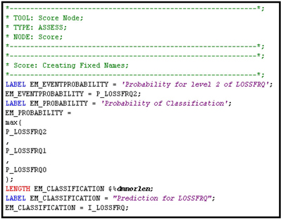
To verify the calculations shown in equations 5.18 – 5.25, run the Neural Network node shown in Display 5.26 and open the Results window. In the Results window, click View→Scoring→SAS Code and scroll down until you see “Writing the Node LOSSFRQ” as shown in Display 5.31.

Display 5.31

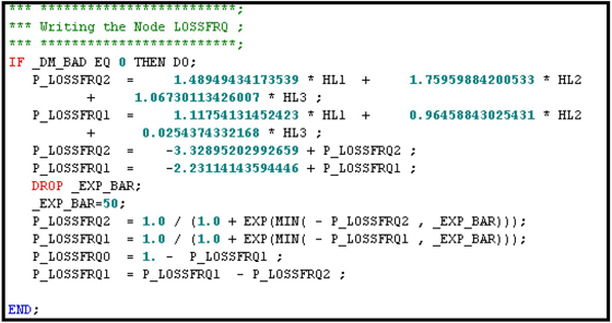
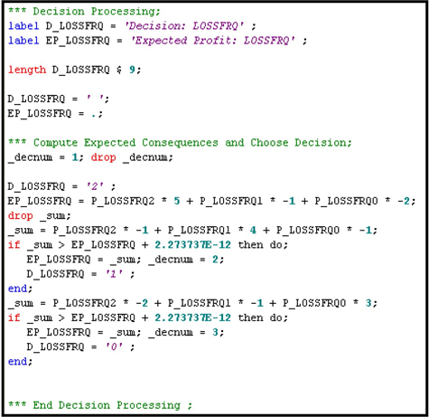
Scroll down further to see how each customer/record is assigned to a risk level using the profit matrix shown in Display 5.28. The steps in assigning a risk level to a customer/record are shown in Display 5.32.

Display 5.32

5.5.1.2 Target Layer Error Function Property

I set this Target Layer Error Function property to MBernoulli. Equation 5.16 is a Bernoulli error function for a binary target. If the target variable (y) takes the values 1 and 0, then the Bernoulli error function is:

E = - 2 \sum i = 1 n {y i ln π ( W , X i ) y i + (1 - y i) ln 1 - π ( W , X i ) 1 - y i}

$E = - 2 \sum_{i = 1}^{n} {y_{i} \ln \frac{π (W, X_{i})}{y_{i}} + (1 - y_{i}) \ln \frac{1 - π (W, X_{i})}{1 - y_{i}}}$

If the target has c mutually exclusive levels (classes), you can create c dummy variables y1,y2,y3,...,yc $y_{1}, y_{2}, y_{3}, ..., y_{c}$ for each record. In this example, the observed loss frequency has the three levels: 0, 1, and 2. These three levels (classes) are mutually exclusive. Hence, I can create three dummy variables y1,y2, and y3 $y_{1}, y_{2}, and y_{3}$ . If the observed loss frequency⁵ is 0 for the ith $i^{t h}$ observation, then yi1=1 $y_{i 1} = 1$ , and both yi2 $y_{i 2}$ and yi3 $y_{i 3}$ are 0. Similarly, if the observed loss frequency is 1, then yi2=1 $y_{i 2} = 1$ , and both yi1 $y_{i 1}$ and yi3 $y_{i 3}$ equals 0. If the observed loss frequency is 2, then yi3=1 $y_{i 3} = 1$ , and the other two dummy variables take on values of 0. This way of representing the target variable by dummy variables is called 1-of-c coding. Using these indicator (dummy) variables, the error function can be written as:

E = - 2 \sum i = 1 n \sum j = 1 c {y i j ln π (W j, X i)}

$E = - 2 \sum_{i = 1}^{n} \sum_{j = 1}^{c} {y_{i j} \ln π (W_{j}, X_{i})}$

where n $n$ is the number of observations in the Training data set and c $c$ is the number of mutually exclusive target levels.⁶

The weights Wj for the jth $W_{j} for the j^{t h}$ level of the target variable are chosen so as to minimize the error function. The minimization is achieved by means of an iterative process. At each iteration, a set of weights is generated, each set defining a candidate model. The iteration stops when the error is minimized or the threshold number of iterations is reached. The next task in the model development process is to select one of these models. This is done by applying the Model Selection Criterion property to the Validation data set.

5.5.1.3 Model Selection Criterion Property

I set the Model Selection Criterion property to Average Error. During the training process, the Neural Network node creates a number of candidate models, one at each iteration. If we set Model Selection Criterion to Average Error, the Neural Network node selects the model that has the smallest error calculated using the Validation data set.

5.5.1.4 Score Ranks in the Results Window

Open the Results window of the Neural Network node to see the details of the selected model.

The Results window is shown in Display 5.33.

Display 5.33

The score rankings are shown in the Score Rankings window. To see how lift and cumulative lift are presented for a model with an ordinal target, you can open the table corresponding to the graph by clicking on the Score Rankings window, and then clicking on the Table icon on the task bar. Selected columns from the table behind the Score Rankings graph are shown in Display 5.34.

Display 5.34

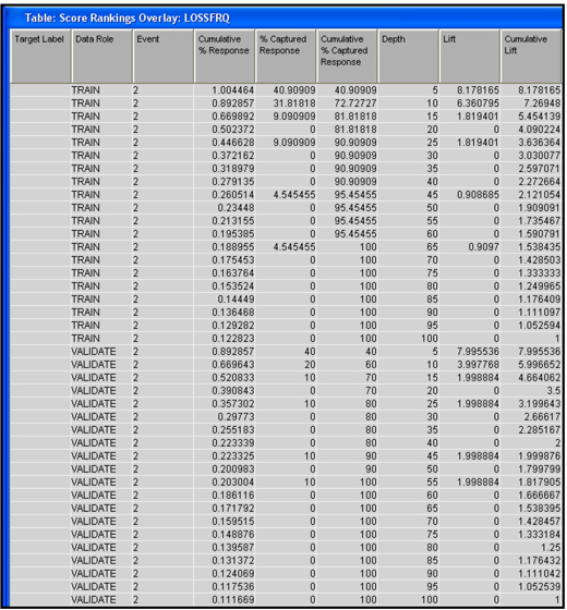
In Display 5.34, column 3 has the title Event. This column has a value of 2 for all rows. You can infer that SAS Enterprise Miner created the lift charts for the target level 2, which is the highest level for the target variable LOSSFRQ.

When the target is ordinal, SAS Enterprise Miner creates lift charts based on the probability of the highest level of the target variable. For each record in the test data set, SAS Enterprise Miner computes the predicted or posterior probability Pr(lossfrq=2|Xi) $P r (l o s s f r q = 2 | X_{i})$ from the model. Then it sorts the data set in descending order of the predicted probability and divides the data set into 20 percentiles (bins).⁷ Within each percentile it calculates the proportion of cases with actual lossfrq $l o s s f r q$ = 2. The lift for a percentile is the ratio of the proportion of cases with lossfrq $l o s s f r q$ = 2 in the percentile to the proportion of cases with lossfrq $l o s s f r q$ =2 in the entire data set.

To assess model performance, the insurance company must rank its customers by the expected value of LOSSFRQ $L O S S F R Q$ , instead of the highest level of the target variable. To demonstrate how to construct a lift table based on expected value of the target, I construct the expected value for each record in the data set by using the following formula.

E (l o s s f r q | X i) = P r (l o s s f r q = 0 | X i) * 0 + P r (l o s s f r q = 1 | X i) * 1 + P r (l o s s f r q = 2 | X i) * 2

$E (l o s s f r q | X_{i}) = P r (l o s s f r q = 0 | X_{i}) * 0 + P r (l o s s f r q = 1 | X_{i}) * 1 + P r (l o s s f r q = 2 | X_{i}) * 2$

Then I sorted the data set in descending order of E(lossfrq|Xi) $E (l o s s f r q | X_{i})$ , and divided the data set into 20 percentiles. Within each percentile, I calculated the mean of the actual or observed value of the target variable lossfrq $l o s s f r q$ . The ratio of the mean of actual lossfrq $l o s s f r q$ in a percentile to the overall mean of actual lossfrq $l o s s f r q$ for the data set is the lift of the percentile.

These calculations were done in the SAS Code node, which is connected to the Neural Network node as shown Display 5.26.

The SAS program used in the SAS Code node is shown in Displays 5.88, 5.89, and 5.90 in the appendix to this chapter.

The lift tables based on E(lossfrq|Xi) $E (l o s s f r q | X_{i})$ are shown in Tables 5.9, 5.10, and 5.11.

Table 5.9

Table 5.10

Table 5.11

5.5.2 Scoring a New Dataset with the Model

The Neural Network model we developed can be used for scoring a data set where the value of the target is not known. The Score node uses the model developed by the Neural Network node to predict the target levels and their probabilities for the Score data set.

Display 5.26 shows the process flow for scoring. The process flow consists of an Input Data node called Ch5_LOSSDAT_SCORE2, which reads the data set to be scored. The Score node in the process flow takes the model score code generated by the Neural Network node and applies it to the data set to be scored.

The output generated by the Score node includes the predicted (assigned) levels of the target and their probabilities. These calculations reflect the solution of Equations 5.18 through 5.25.

Display 5.35 shows the programming statements used by the Score node to calculate the predicted probabilities of the target levels.

Display 5.35

Display 5.36 shows the assignment of the target levels to individual records using the profit matrix.

Display 5.36

The following code segments create additional variables. Display 5.37 shows the target level assignment process. The variable I_LOSSFRQ is created according to the posterior probability found for each record.

Display 5.37

In Display 5.38, the variable EM_CLASSIFICATION represents predicted values based on maximum posterior probability. EM_CLASSIFICATION is the same as I_LOSSFRQ shown in Display 5.37.

Display 5.38

Display 5.39 shows the list of variables created by the Score node using the Neural Network model.

Display 5.39

5.5.3 Classification of Risks for Rate Setting in Auto Insurance with Predicted Probabilities

The probabilities generated by the neural network model can be used to classify risk for two purposes:

• to select new customers

• to determine premiums to be charged according to the predicted risk

For each record in the data set, you can compute the expected LOSSFRQ as:

E(lossfrq|Xi)=Pr(lossfrq=0|Xi)*0+Pr(lossfrq=1|Xi)*1+Pr(lossfrq=2|Xi)*2 $E (l o s s f r q | X_{i}) = P r (l o s s f r q = 0 | X_{i}) * 0 + P r (l o s s f r q = 1 | X_{i}) * 1 + P r (l o s s f r q = 2 | X_{i}) * 2$ . Customers can be ranked by this expected frequency and assigned to different risk groups.

5.6 Alternative Specifications of the Neural Networks

The general Neural Network model presented in section 5.2 consists of linear combinations functions (Equations 5.1, 5.3, 5.5, 5.7, 5.9, and 5.11) and hyperbolic tangent activation functions (Equations 5.2, 5.4, 5.6, 5.8, 5.10, and 5.12) in the hidden layers, and a linear combination function (Equation 5.13) and a logistic activation function (Equation 5.14) in the output layer. Networks of the type presented in Equations 5.1-5.14 are called multilayer perceptrons and use linear combination functions and sigmoid activation functions in the hidden layers. Sigmoid activation functions are S-shaped, and they are shown in Displays 5.0B, 5.0C, 5.0D and 5.0E.

In this section, I introduce you to other types of networks known as Radial Basis Function (RBF) networks, which have different types of combination activation functions. You can build both Multilayer Perceptron (MLP) networks and RBF networks using the Neural Network node.

5.6.1 A Multilayer Perceptron (MLP) Neural Network

The neural network presented in Equations 5.1-5.14 have two hidden layers. The examples considered here have only one hidden layer with three hidden units. The Neural Network node allows 1–64 hidden units. You can compare the models produced by setting the Number of Hidden Units property to different values and pick the optimum values.

In an MLP neural network the hidden layer combination functions are linear, as shown in Equations 5.26, 5.28, and 5.30. The hidden Layer Activations Functions are sigmoid functions, as shown in Equations 5.27, 5.29, and 5.31.

Hidden Layer Combination Function, Unit 1:

The following equation is the weighted sum of inputs:

η i 1 = b 1 + w 11 x i 1 + w 21 x i 2 + ... + w p 1 x i p (5.26)

$η_{i 1} = b_{1} + w_{11} x_{i 1} + w_{21} x_{i 2} + ... + w_{p 1} x_{i p} (5.26)$

w11xi1+w21xi2+...+wp1xip $w_{11} x_{i 1} + w_{21} x_{i 2} + ... + w_{p 1} x_{i p}$ is the inner product of the weight and input vectors, where w11,w21,......wp1 $w_{11}, w_{21}, ...... w_{p 1}$ are the weights to be estimated by the iterative algorithm of the Neural Network node. The coefficient b1 $b_{1}$ (called bias) is also estimated by the algorithm. Equation 5.26 shows that the combination functions ηi1 $η_{i 1}$ is a weighted sum of the inputs plus bias. The neural network algorithm calculates ηi1 $η_{i 1}$ for the ith $i^{t h}$ person or record at each iteration.

Hidden Layer Activation Function, Unit 1:

The Hidden Layer Activation Function in an MLP network is a sigmoid function such as the Hyperbolic Tangent, Arc Tangent, Elliot, or Logistic. The sigmoid functions are S-shaped, as shown in Displays 5.0B – 5.0E.

Equation 5.27 shows a sigmoid function known as the tanh function.

H i 1 = tanh (η i 1) = exp ( η i 1 ) - exp ( - η i 1 ) exp ( η i 1 ) + exp ( - η i 1 ) (5.27)

$H_{i 1} = \tanh (η_{i 1}) = \frac{\exp (η_{i 1}) - \exp (- η_{i 1})}{\exp (η_{i 1}) + \exp (- η_{i 1})} (5.27)$

The neural network algorithm calculates Hi1 $H_{i 1}$ for the ith $i^{t h}$ case or record at each iteration.

Hidden Layer Combination Function, Unit 2:

η i 2 = b 2 + w 12 x i 1 + w 22 x i 2 + ... + w p 2 x i p (5.28)

$η_{i 2} = b_{2} + w_{12} x_{i 1} + w_{22} x_{i 2} + ... + w_{p 2} x_{i p} (5.28)$

Hidden Layer Activation Function, Unit 2:

H i 2 = tanh (η i 2) = exp ( η i 2 ) - exp ( - η i 2 ) exp ( η i 2 ) + exp ( - η i 2 ) (5.29)

$H_{i 2} = \tanh (η_{i 2}) = \frac{\exp (η_{i 2}) - \exp (- η_{i 2})}{\exp (η_{i 2}) + \exp (- η_{i 2})} (5.29)$

Hidden Layer Combination Function, Unit 3:

η i 3 = b 3 + w 13 x i 1 + w 23 x i 2 + ... + w p 3 x i p (5.30)

$η_{i 3} = b_{3} + w_{13} x_{i 1} + w_{23} x_{i 2} + ... + w_{p 3} x_{i p} (5.30)$

Hidden Layer Activation Function, Unit 3:

H i 3 = tanh (η i 3) = exp ( η i 3 ) - exp ( - η i 3 ) exp ( η i 3 ) + exp ( - η i 3 ) (5.31)

$H_{i 3} = \tanh (η_{i 3}) = \frac{\exp (η_{i 3}) - \exp (- η_{i 3})}{\exp (η_{i 3}) + \exp (- η_{i 3})} (5.31)$

Target Layer Combination Function:

η i = b + w 1 H i 1 + w 2 H i 2 + w 3 H i 3 (5.32)

$η_{i} = b + w_{1} H_{i 1} + w_{2} H_{i 2} + w_{3} H_{i 3} (5.32)$

Target Layer Activation Function:

1 1 + E X P ( - η i )

$\frac{1}{1 + E X P (- η_{i})}$

If the target is binary, then the target layer output is

P (Target=1) = 1 1 + E X P ( - η i ) and

$P (Target=1) = \frac{1}{1 + E X P (- η_{i})} and$

P (Target=0) = 1 1 + E X P ( η i )

$P (Target=0) = \frac{1}{1 + E X P (η_{i})}$

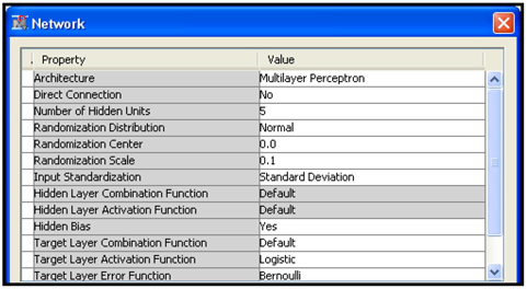
If you want to use a built-in MLP network, click located at the right of the Network property of the Neural Network node. Set the Architecture property to Multilayer Perceptron in the Network Properties window, as shown in Display 5.40.

Display 5.40

When you set the Architecture property to Multilayer Perceptron, the Neural Network node uses the default values Linear and Tanh for the Hidden Layer Combination Function and the Hidden Layer Activation Function properties. The default values for the Target Layer Combination Function and Target Layer Activation Function properties are Linear and Exponential. You can change the Target Layer Combination Function, Target Layer Activation Function, and Target Layer Error Function properties. I changed the Target Layer Activation Function property to Logistic, as shown in Display 5.40. If the Target is Binary and the Target Layer Activation Function is Logistic, then you can set the Target Layer Error Function property to Bernoulli to generate a Logistic Regression-type model.

5.6.2 A Radial Basis Function (RBF) Neural Network

The Radial Basis Function neural network can be represented by the following equation:

y i = \sum k = 1 M w k ϕ k (X i) + w 0 (5.33)

$y_{i} = \sum_{k = 1}^{M} w_{k} ϕ_{k} (X_{i}) + w_{0} (5.33)$

where yi $y_{i}$ is the target variable for ith $i^{t h}$ case (record or observation), wk $w_{k}$ is the weight for the kth $k^{t h}$ basis function, w0 $w_{0}$ is the bias, ϕk $ϕ_{k}$ is the kth $k^{t h}$ basis function, Xi=(xi1,xi2,.......,xip) $X_{i} = (x_{i 1}, x_{i 2}, ......., x_{i p})$ is a vector of inputs for the ith $i^{t h}$ case, M $M$ is the number of basis functions, p $p$ is the number of inputs, and N $N$ is the number of cases (observations) in the Training data set. The weight multiplied by the basis function plus the bias can be thought of as the output of a hidden unit in a single layer network.

An example of a basis function is:

ϕk(Xi)=exp(−∥Xi−μk∥2σk) $ϕ_{k} (X_{i}) = \exp (- \frac{‖ X_{i} - μ_{k} ‖}{2 σ_{k}})$ , where Xi=(xi1,xi2,.......,xip) $X_{i} = (x_{i 1}, x_{i 2}, ......., x_{i p})$ , μk=(μ1k,μ2k,.......,μpk) $μ_{k} = (μ_{1 k}, μ_{2 k}, ......., μ_{p k})$ , i stands for the ith $i stands for the i^{t h}$ observation and k stands for the kth $k stands for the k^{t h}$ basis function. ∥Xi−μk∥ $‖ X_{i} - μ_{k} ‖$ is the Squared Euclidean distance between the vectors Xi $X_{i}$ and μk $μ_{k}$ . μk $μ_{k}$ and σk $σ_{k}$ are the center and width of the kth $k^{t h}$ basis function. The values of the center and width are determined during the training process.

5.6.2.1 Radial Basis Function Neural Networks in the Neural Network Node

An alternative way of representing a Radial Basis neural network is by using the equation:

y i = \sum k = 1 M w k H i k + w 0 (5.33 A)

$y_{i} = \sum_{k = 1}^{M} w_{k} H_{i k} + w_{0} (5.33 A)$

where Hik $H_{i k}$ is the output of the kth $k^{t h}$ hidden unit for the ith $i^{t h}$ observation (case) , M $M$ is the number of hidden units, wk $w_{k}$ is the weight for the kth $k^{t h}$ hidden unit, w0 $w_{0}$ is the bias, and yi $y_{i}$ is the target value for the ith $i^{t h}$ observation (case).

The following examples show how the outputs of the hidden units are calculated for different types of Basis Functions, and how the target values are computed. In each case the formulas are followed by SAS code. The output of the target layer is yi $y_{i}$ . The number of output units in the target layer can be more than one, depending on your target variable. For example, if the target is binary, then the target layer calculates two outputs, namely P_resp1 and P_resp0, for each observation, where P_resp1=Pr(resp=1) $\Pr (r e s p = 1)$ and P_resp0 = Pr(resp=0) $\Pr (r e s p = 0)$ .

As shown by Equations 5.26, 5.28, and 5.30, the hidden layer combination function in a MLP neural network is the weighted sum or inner product of the vector of inputs and vector of corresponding weights plus a bias coefficient.

In contrast to the Hidden Layer Combination function in an MLP neural network, the hidden layer combination function in a RBF neural network is the Squared Euclidian Distance between the vector of inputs and the vector of corresponding weights (center points), multiplied by squared bias.

In the Neural Network node, the Basis functions are defined in terms of the combination and activation functions of the hidden units.

An example of a combination function used in some RBF networks is

η i k = - b k 2 \sum j = 1 p (w j k - x i j) 2 (5.34)

$η_{i k} = - b_{k}^{2} \sum_{j = 1}^{p} {(w_{j k} - x_{i j})}^{2} (5.34)$

where ηik $η_{i k}$ = the estimated value of the combination function for the kth $k^{t h}$ hidden unit

bk $b_{k}$ = bias,

wjk $w_{j k}$ = weight of the jth $j^{t h}$ input

xij $x_{i j}$ = jth $j^{t h}$ input

i $i$ = ith $i^{t h}$ record or observation in the data set

p $p$ = the number of inputs

The RBF neural network which uses the combination function given by equation 5.34 is called the Ordinary Radial with Unequal Widths or ORBFUN.

The activation function of the hidden units of an ORBFUN network is an exponential function. Hence the output of kth $k^{t h}$ hidden unit in ORBFUN network is:

H i k = E x p ⎧ ⎩ ⎨ - b k 2 \sum j p (w j k - x i j) 2 ⎫ ⎭ ⎬ (5.35)

$H_{i k} = E x p {- b_{k}^{2} \sum_{j}^{p} {(w_{j k} - x_{i j})}^{2}} (5.35)$

As Equation 5.35 shows, the bias is not the same in all the units in the hidden layer. Since the width $w i d t h$ is inversely related to the bias bk $b_{k}$ (bk=1σk $b_{k} = \frac{1}{σ_{k}}$ ), it is also different for different units. Hence the term Unequal Widths in ORBFUN.

The network with the combination function given in Equation 5.34 and the activation function given in Equation 5.35 is called the Ordinary Radial with Unequal Widths or ORBFUN.

To build an ORBFUN neural network model, click located to the right of the Network property of the Neural Network node. In the Network window that opens, set the Architecture Property to Ordinary Radial-Unequal Width, as shown in Display 5.41.

Display 5.41

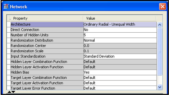
As you can see in Display 5.41, the rows corresponding to Hidden Layer Combination Function and Hidden Layer Activation Function are shaded, indicating that their values are fixed for this network. Hence this is called a built-in network in SAS Enterprise Miner terminology. However, the rows corresponding to the Target Layer Combination Function, Target Layer Activation Function, and Target Layer Error Function are not shaded, so you can change their values. For example, to set the Target Layer Activation Function to Logistic, click on the value column corresponding to Target Layer Activation Function property and select Logistic. Similarly you can change the Target Layer Error Function to Bernoulli.

As pointed out earlier in this chapter, the error function you select depends on the type of model you want to build.

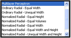
Display 5.42 shows a list of RBF neural networks available in SAS Enterprise Miner. You can see all the network architectures If you click on the down-arrow in the box to the right of the Architecture property in the Network window.

Display 5.42

For a complete description of these network architectures, see SAS Enterprise Miner: Reference Help, which is available in the SAS Enterprise Miner Help. In the following pages I will review some of the RBF network architectures.

The general form of the Hidden Layer Combination Function of a RBF network is:

η k = f * log (a b s (a k)) - b k 2 \sum j p (w j k - x j) 2 (5.36)

$η_{k} = f * \log (a b s (a_{k})) - b_{k}^{2} \sum_{j}^{p} {(w_{j k} - x_{j})}^{2} (5.36)$

The Hidden Layer Activation Function is

H k = exp (η k) (5.37)

$H_{k} = \exp (η_{k}) (5.37)$

and where xj $x_{j}$ is the jth $j^{t h}$ standardized input, the wjk's $w_{j k}' s$ are weights representing the center (origin) of the basis function, ak $a_{k}$ is the height, or altitude, bk $b_{k}$ is a parameter sometimes referred to as the bias, p $p$ is the number of inputs, f $f$ is the number of connections to the unit and k $k$ refers to the kth $k^{t h}$ hidden unit. Another measure that is related to bias is the width. The bias bk $b_{k}$ is the inverse width of the kth $k^{t h}$ hidden unit. (see the section “Definitions for Built-in Architectures” in SAS Enterprise Miner: Reference Help, which is available in the SAS Enterprise Miner Help). The coefficient ak $a_{k}$ , called the height parameter, measures the maximum height of the bell-shaped curve presented in Displays 5.43 through 5.45. The subscript k $k$ is added to indicate that the radial basis function is used to calculate the output of the kth $k^{t h}$ hidden unit. Although Equations 5.36 and 5.37 are evaluated for each observation during the training of the neural network, I have dropped the subscript i $i$ , which I used in Equations 5.34 and 5.35 to denote the ith $i^{t h}$ record.

When there are p $p$ inputs, there are p $p$ weights. These weights are estimated by the Neural Network node. The vector of inputs for any record or observation may be thought of as a point in p-dimensional space in which the vector of weights is the center. Given the height and width, the value of the radial basis function depends on the distance between the inputs and the center.

Now I plot the radial basis functions with different heights and widths for a single input that ranges between –10 and 10. Since there is only input, there is only one weight w1k $w_{1 k}$ , which I arbitrarily set to 0.

Display 5.43 shows a graph of the radial basis function given in Equations 5.36 and 5.37 with height = 1 and width = 1.

Display 5.43

Display 5.44 shows a graph of the radial basis function given in Equation 5.36 with height = 1 and width = 4.

Display 5.44

Display 5.45 shows a graph of the radial basis function given in Equation 5.36 with height = 5 and width = 4.

Display 5.45

If there are three units in a hidden layer, each having a radial basis function, and if the radial basis functions are constrained to sum to 1, then they are called Normalized Radial Basis Functions in SAS Enterprise Miner. Without this constraint, they are called Ordinary Radial Basis Functions.

5.7 Comparison of Alternative Built-in Architectures of the Neural Network Node

You can produce a number of neural network models by specifying alternative architectures in the Neural Network node. You can then make a selection from among these models, based on lift or other measures, using the Model Comparison node. In this section, I compare the built-in architectures listed in the Display 5.46.

Display 5.46

Display 5.47 shows the process flow diagram for comparing the Neural Network models produced by different architectural specifications. In all the eight models compared in this section, I set the Assessment property to Average Error and the Number of Hidden Units property to 5.

Display 5.47

5.7.1 Multilayer Perceptron (MLP) Network

The top Neural Network node in Display 5.47 is a MLP network, and its property settings are shown in Display 5.48.

Display 5.48

The default value of the Hidden Layer Combination Function property is Linear and the default value of the Hidden Layer Activation Functions property is Tanh. After running this node, you can open the Results window and view the SAS code generated by the Neural Network node. Display 5.49 shows a segment of the SAS code generated by the Neural Network mode with the Network settings shown in Display 5.48.

Display 5.49

The code segment shown in Display 5.50 shows that the final outputs in the Target Layer are computed using a Logistic Activation Function.

Display 5.50

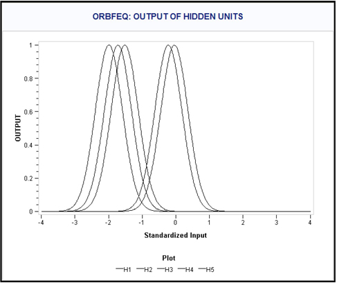
5.7.2 Ordinary Radial Basis Function with Equal Heights and Widths (ORBFEQ)

The combination function for the kth $k^{t h}$ Hidden Unit in this case is ηk=−b2∑j=1p(wjk−xj)2 $η_{k} = - b^{2} \sum_{j = 1}^{p} {(w_{j k} - x_{j})}^{2}$ and the Activation function for the kth $k^{t h}$ hidden unit is given by Hk=exp(ηk). $H_{k} = \exp (η_{k}) .$ Note that the parameter b $b$ in the Combination function above is constant for all the hidden units. Display 5.51 shows an example of the outputs of five Hidden Units of an ORBFEQ with a single input.

Display 5.51

In the second Neural Network node in Display 5.47, the Architecture property is set to Ordinary Radial – Equal width as shown in Display 5.52.

Display 5.52

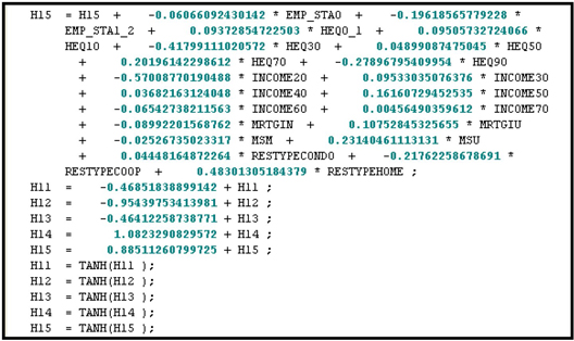
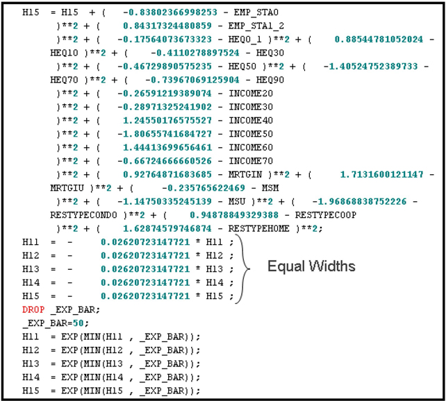
Display 5.53 shows a segment of the SAS code, which shows the computation of the outputs of the hidden units of the ORBFEQ neural network specified in Display 5.52.

Display 5.53

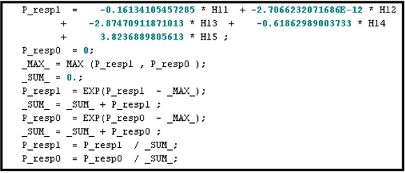
Display 5.54 shows the computation of the outputs of the target layer of the ORBFEQ neural network specified in Display 5.52.

Display 5.54

5.7.3 Ordinary Radial Basis Function with Equal Heights and Unequal Widths (ORBFUN)

In this network, the combination function for the kth $k^{t h}$ unit is ηk=−bk2∑j=1p(wjk−xj)2, $η_{k} = - b_{k}^{2} \sum_{j = 1}^{p} {(w_{j k} - x_{j})}^{2},$ where wjk $w_{j k}$ are the weights iteratively calculated by the Neural Network node, xj $x_{j}$ is the jth $j^{t h}$ input (standardized), and bk $b_{k}$ is the reciprocal of the width for the kth $k^{t h}$ hidden unit. Unlike the ORBFEQ example in which a single value for b is calculated to be used with all the hidden units, the constant bk $b_{k}$ in this case can differ from one hidden unit to another. The output of the kth $k^{t h}$ hidden unit is given by Hk=exp(ηk). $H_{k} = \exp (η_{k}) .$

Display 5.55shows an example of the output of the five hidden units Hk(k=1,2,3,4 and 5) $H_{k} (k = 1, 2, 3,4 and 5)$ with a single standardized input and arbitrary values for wjk $w_{j k}$ and bk. $b_{k} .$

Display 5.55

The Architecture property of the ORBFUN Neural Network node (the third node from the top in Display 5.46) is set to Ordinary Radial – Unequal Width. The remaining Network properties are the same as in Display 5.52.

Displays 5.56 and 5.57 show the SAS code segment showing the calculation of the outputs of the hidden and target layers of this ORBFUN network.

Display 5.56

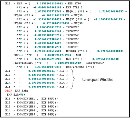
Display 5.57

5.7.4 Normalized Radial Basis Function with Equal Widths and Heights (NRBFEQ)

In this case, the combination function for the kth $k^{t h}$ hidden unit is ηk=−b2∑j=1p(wjk−xj)2, $η_{k} = - b^{2} \sum_{j = 1}^{p} {(w_{j k} - x_{j})}^{2},$ where wjk $w_{j k}$ are the weights iteratively calculated by the Neural Network node, xj $x_{j}$ is the jth $j^{t h}$ input (standardized), and b $b$ is the square root of the reciprocal of the width. The height kth $k^{t h}$ hidden unit is = ak=1. $a_{k} = 1.$ Since log(1)=0, $\log (1) = 0,$ it does not appear in the combination function shown above. Here it is implied that f=1 $f = 1$ (See equation 5.36).

The output of the kth $k^{t h}$ hidden unit is given by Hk=exp(ηk)∑m=15exp(ηm) $H_{k} = \frac{\exp (η_{k})}{\sum_{m = 1}^{5} \exp (η_{m})}$ . This is called the

Softmax Activation Function. Display 5.58 shows the output of the five hidden units Hk(k=1,2,3,4 and 5) $H_{k} (k = 1, 2, 3, 4 and 5)$ with a single standardized input, and arbitrary values for wjk $w_{j k}$ and b. $b .$

In this case, the height ak $a_{k}$ =1 for all the hidden units. Hence log(ak)=0 $\log (a_{k}) = 0$ .

Display 5.58

For a NRBFEQ neural network, the Architecture property is set to Normalized Radial – Equal Width and Height. The remaining Network settings are the same as in Display 5.52.

Displays 5.59 and 5.60 show segments from the SAS code generated by the Neural Network node. Display 5.59 shows the computation of the outputs of the hidden units and Display 5.60 shows the calculation of the target layer outputs.

Display 5.59

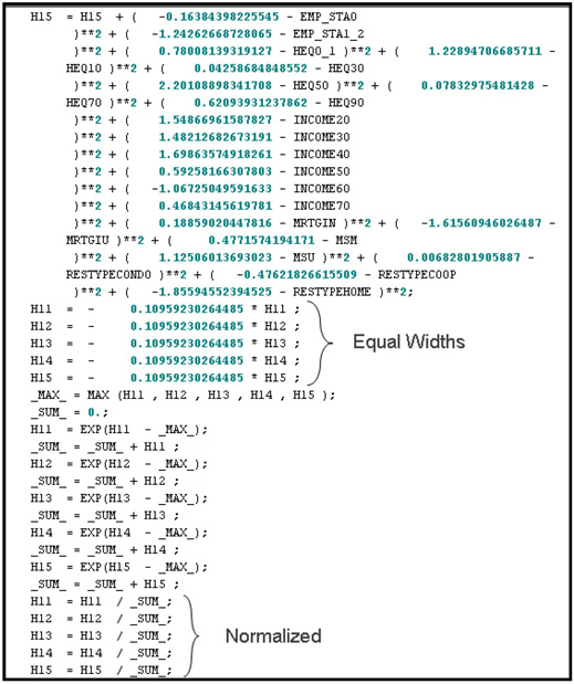
Display 5.60

5.7.5 Normalized Radial Basis Function with Equal Heights and Unequal Widths (NRBFEH)

The combination function here is ηk=−bk2∑j=1p(wjk−xj)2, $η_{k} = - b_{k}^{2} \sum_{j = 1}^{p} {(w_{j k} - x_{j})}^{2},$ where wjk $w_{j k}$ the weights are iteratively calculated by the Neural Network node, xj $x_{j}$ is the jth $j^{t h}$ input (standardized), and bk $b_{k}$ is the reciprocal of the width for the kth $k^{t h}$ hidden unit. The output of the kth $k^{t h}$ hidden unit is given by Hk=exp(ηk)∑m=15exp(ηm) $H_{k} = \frac{\exp (η_{k})}{\sum_{m = 1}^{5} \exp (η_{m})}$ .

Display 5.61 shows the output of the five hidden units Hk(k=1,2,3,4 and 5) $H_{k} (k = 1, 2, 3, 4 and 5)$ with a single standardized input AGE (p $p$ =1), and arbitrary values for wjk $w_{j k}$ and bk $b_{k}$ . The height ak $a_{k}$ =1 for all the hidden units. Hence log(ak)=0 $\log (a_{k}) = 0$ .

Display 5.61

The Architecture property for the NRBFEH neural network is set to Normalized Radial – Equal Height. The remaining Network settings are the same as in Display 5.52.

Display 5.62 shows a segment of the SAS code used to compute the hidden units in this NRBEH network.

Display 5.62

Display 5.63 shows the SAS code used to compute the target layer outputs.

Display 5.63

5.7.6 Normalized Radial Basis Function with Equal Widths and Unequal Heights (NRBFEW)

The combination function in this case is:

ηk=f*log(abs(ak))−b2∑jp(wjk−xj)2, $η_{k} = f * \log (a b s (a_{k})) - b^{2} \sum_{j}^{p} {(w_{j k} - x_{j})}^{2},$ where ak $a_{k}$ is an altitude parameter representing the maximum height, f $f$ is the number of connections to the unit, and b $b$ is the square root of reciprocal of the width.

The output of the kth $k^{t h}$ hidden unit is given by Hk=exp(ηk)∑m=15exp(ηm) $H_{k} = \frac{\exp (η_{k})}{\sum_{m = 1}^{5} \exp (η_{m})}$ .

Display 5.64 shows the output of the five hidden units Hk(k=1,2, 3,4 and 5) $H_{k} (k = 1, 2, 3,4 and 5)$ with a single standardized input and arbitrary values for wjk $w_{j k}$ , ak $a_{k}$ , and b. $b .$

Display 5.64

The Architecture property of the estimated NRBFEW network is set to Normalized Radial – Equal Width. The remaining Network settings are the same as in Display 5.52.

Display 5.65 shows the code segment showing the calculation of the output of the hidden units in the estimated NRBFEW network.

Display 5.65

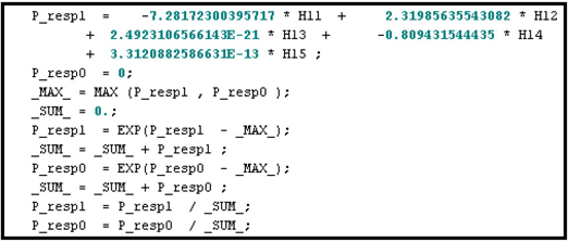
Display 5.66 shows the calculation of the outputs of the target layer.

Display 5.66

5.7.7 Normalized Radial Basis Function with Equal Volumes (NRBFEV)

In this case, the combination function is:

η k = f * log (a b s (b k)) - b k 2 \sum j p (w j k - x j) 2

$η_{k} = f * \log (a b s (b_{k})) - b_{k}^{2} \sum_{j}^{p} {(w_{j k} - x_{j})}^{2}$

The output of the jth $j^{t h}$ hidden unit is given by Hk=exp(ηk)∑m=15exp(ηm) $H_{k} = \frac{\exp (η_{k})}{\sum_{m = 1}^{5} \exp (η_{m})}$ .

Display 5.67 shows the output of the five hidden units Hk(k=1,2,3,4 and 5) $H_{k} (k = 1, 2, 3, 4 and 5)$ with a single standardized input, and arbitrary values for wjk $w_{j k}$ and bk. $b_{k} .$

Display 5.67

The Architecture property of the NRBFEV architecture used in this example is set to Normalized Radial – Equal Volumes. The remaining Network settings are the same as in Display 5.52.

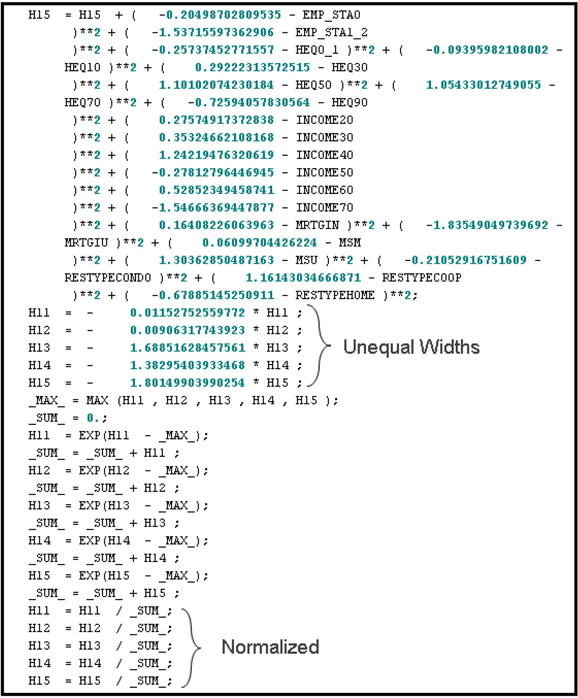
Display 5.68 shows a segment of the SAS code generated by the Neural Network node for the NRBFEV network.

Display 5.68

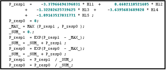
Display 5.69 shows the computation of the outputs of the target layer in the estimated NRBFEV network.

Display 5.69

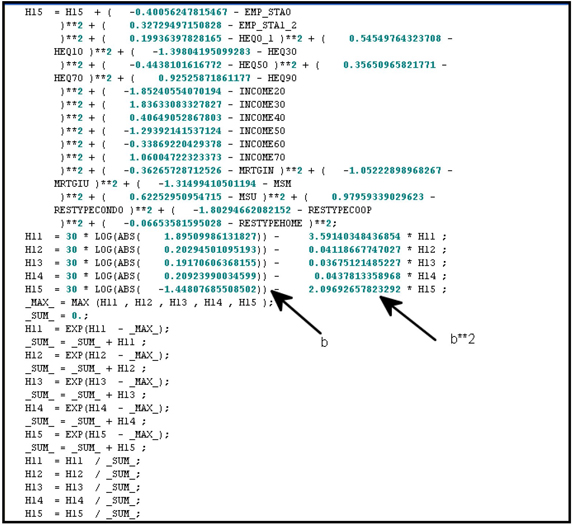
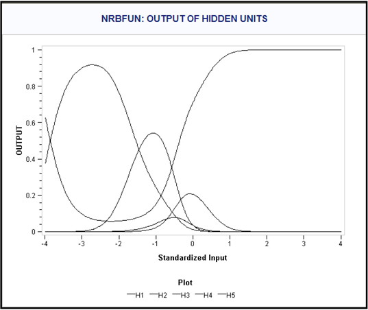
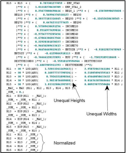
5.7.8 Normalized Radial Basis Function with Unequal Widths and Heights (NRBFUN)

Here, the combination function for the kth $k^{t h}$ hidden unit is:

ηk=f*log(abs(ak))−bk2∑ip(wjk−xj)2, $η_{k} = f * \log (a b s (a_{k})) - b_{k}^{2} \sum_{i}^{p} {(w_{j k} - x_{j})}^{2},$ where ak $a_{k}$ is the altitude and bk $b_{k}$ is the reciprocal of the width.

The output of the kth $k^{t h}$ hidden unit is given by Hk=exp(ηk)∑m=15exp(ηm) $H_{k} = \frac{\exp (η_{k})}{\sum_{m = 1}^{5} \exp (η_{m})}$ .

Display 5.70 shows the output of the five hidden units Hk(k=1,2,3,4 and 5) $H_{k} (k = 1, 2, 3, 4 and 5)$ with a single standardized input and arbitrary values for wjk $w_{j k}$ , ak $a_{k}$ , and bk. $b_{k} .$

Display 5.70

The Architecture property for the NRBFUN network is set to Normalized Radial – Unequal Width and Height. The remaining Network settings are the same as in Display 5.52.

Display 5.71 shows the segment of the SAS code used for calculating the outputs of the hidden units.

Display 5.71

Display 5.72 shows the SAS code needed for calculating the outputs of the target layer of the NRBFUN network.

Display 5.72

5.7.9 User-Specified Architectures

With the user-specified Architecture setting, you can pair different Combination Functions and Activation Functions. Each pair generates a different Neural Network model, and all possible pairs can produce a large number of Neural Network models.

You can select the following settings for the Hidden Layer Activation Function:

• ArcTan

• Elliott

• Hyperbolic Tangent

• Logistic

• Gauss

• Sine

• Cosine

• Exponential

• Square

• Reciprocal

• Softmax

You can select the following settings for the Hidden Layer Combination Function:

• Add

• Linear

• EQSlopes

• EQRadial

• EHRadial

• EWRadial

• EVRadial

• XRadial

5.7.9.1 Linear Combination Function with Different Activation Functions for the Hidden Layer

Begin by setting the Architecture property to User, the Target Layer Combination Function property to Default, and the Target Layer Activation Function property to Default. In addition, set the Hidden Layer Combination Function property to Linear, the Input Standardization property to Standard Deviation, and the Hidden Layer Activation Function property to one of the available values.

If you set the Hidden Layer Combination Function property to Linear, the output of the kth $k^{t h}$ hidden layer is estimated by Equation 5.38 for the kth $k^{t h}$ hidden unit.

η k = w 0 k + \sum j = 1 p w j k x j (5.38)

$η_{k} = w_{0 k} + \sum_{j = 1}^{p} w_{j k} x_{j} (5.38)$

where w1k,w2k,....wpk $w_{1 k}, w_{2 k,} .... w_{p k}$ are the weights, x1,x2,...xp $x_{1}, x_{2}, ... x_{p}$ are the standardized inputs,⁸ and w0k $w_{0 k}$ is the bias coefficient. You can use the Hidden Layer Combination Function given by equation 5.38 with each of the following Hidden Layer Activation Functions.

Arc Tan	Hk=(2/π)tan−1(ηk) $H_{k} = (2 / π) \tan^{- 1} (η_{k})$
Elliot	Hk=ηk1+\|ηk\| $H_{k} = \frac{η_{k}}{1 + \| η_{k} \|}$
Hyperbolic Tangent	Hk=tanh(ηk) $H_{k} = \tanh (η_{k})$
Logistic	Hk=11+exp(−ηk) $H_{k} = \frac{1}{1 + \exp (- η_{k})}$
Gauss	Hk=exp(−0.5η2k) $H_{k} = \exp (- 0.5 η^{2}_{k})$
Sine	Hk=sin(ηk) $H_{k} = \sin (η_{k})$
Cosine	Hk=cos(ηk) $H_{k} = \cos (η_{k})$
Exponential	Hk=exp(ηk) $H_{k} = \exp (η_{k})$
Square	Hk=ηk2 $H_{k} = η_{k}^{2}$
Reciprocal	$H_{k} = \frac{1}{η_{k}}$
Softmax	$H_{k} = \frac{\exp (η_{k})}{\sum_{j = 1}^{M} \exp (η_{j})}$

$where k = 1, 2, 3, ... M$ and $M$ is the number of hidden units.

The above specifications of the Hidden Layer Activation Function with the Hidden Layer Combination Function shown in equation 5.38 will result in 11 different neural network models.

5.7.9.2 Default Activation Function with Different Combination Functions for the Hidden Layer

You can set the Hidden Layer Combination Function property to the following values. For each item, I show the formula for the combination function for the $k^{t h}$ hidden unit.

Add

$η_{k} = \sum_{j = 1}^{p} x_{j}, where x_{1}, x_{2}, ... x_{p} are the standardized inputs .$

Linear

$η_{k} = w_{0 k} + \sum_{j = 1}^{p} w_{j k} x_{j},$ where $w_{j k}$ is the weight of $j^{t h}$ input in the $k^{t h}$ hidden unit and $w_{0 k}$ is the bias coefficient.

EQSlopes

$η_{k} = w_{0 k} + \sum_{j = 1}^{p} w_{j} x_{j},$ where the $w_{j}$ weights (coefficients) on the inputs do not differ from one hidden unit to the next, though the bias coefficients, given by the $w_{0 k}$ , may differ.

EQRadial

$η_{k} = - b^{2} \sum_{j = 1}^{p} {(w_{j k} - x_{j})}^{2},$ where $x_{j}$ is the $j^{t h}$ standardized input, and $w_{j k}$ and $b$ are calculated iteratively by the Neural Network node. The coefficient $b$ does not differ from one hidden unit to the next.

EHRadial

$η_{k} = - b_{k}^{2} \sum_{j = 1}^{p} {(w_{j k} - x_{j})}^{2},$ where $x_{j}$ is the $j^{t h}$ standardized input, and $w_{j k}$ and $b_{k}$ are calculated iteratively by the Neural Network node.

EWRadial

$η_{k} = f * \log (a b s (a_{k})) - b^{2} \sum_{j}^{p} {(w_{j k} - x_{j})}^{2},$ where $x_{j}$ is the $j^{t h}$ standardized input, $w_{j k}$ , $a_{k}$ , and $b$ are calculated iteratively by the Neural Network node, and $f$ is the number of connections to the unit. In SAS Enterprise Miner, the constant $f$ is called fan-in. The fan-in of a unit is the number of other units, from the preceding layer, feeding into that unit.

EVRadial

$η_{k} = f * \log (a b s (b_{k})) - b_{k}^{2} \sum_{k}^{p} {(w_{j k} - x_{j})}^{2},$ where $w_{i j}$ and $b_{j}$ are calculated iteratively by the Neural Network node, and $f$ is the number of other units feeding in to the unit..

XRadial

$η_{k} = f * \log (a b s (a_{k})) - b_{k}^{2} \sum_{j = 1}^{p} {(w_{j k} - x_{j})}^{2},$ where $w_{i j}$ , $b_{j}$ , and $a_{j}$ are calculated iteratively by the Neural Network node.

5.7.9.3 List of Target Layer Combination Functions for the User-Defined Networks

Add, Linear, EQSlope, EQRadial, EHRadial, EWRadial, EVRadial, and XRadial.

5.7.9.4 List of Target Layer Activation Functions for the User-Defined Networks

Identity, Linear, Exponential, Square, Logistic, and Softmax.

5.8 AutoNeural Node

As its name suggests, the AutoNeural node automatically configures a Neural Network model. It uses default combination functions and error functions. The algorithm tests different activation functions and selects the one that is optimum.

Display 5.73 shows the property settings of the AutoNeural node used in this example. Segments of SAS code generated by AutoNeural node are shown in Displays 5.74 and 5.75.

Display 5.73

Display 5.74 shows the computation of outputs of the hidden units in the selected model.

Display 5.74

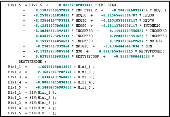
From Display 5.74 it is clear that in the selected model inputs are combined using a Linear Combination Function in the hidden layer. A Sin Activation Function is applied to calculate the outputs of the hidden units.

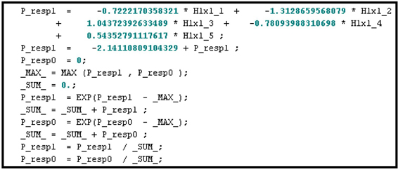
Display 5.75 shows the calculation of the outputs of the Target layer.

Display 5.75

5.9 DMNeural Node

DMNeural node fits a non linear equation using bucketed principal components as inputs. The model derives the principal components from the inputs in the training data set. As explained in Chapter 2, the principal components are weighted sums of the original inputs, the weights being the eigenvectors of the variance covariance or correlation matrix of the inputs. Since each observation has a set of inputs, you can construct a Principal Component value for each observation from the inputs of that observation. The Principal components can be viewed as new variables constructed from the original inputs.

The DMNeural node selects the best principal components using the R-square criterion in a linear regression of the target variable on the principal components. The selected principal components are then binned or bucketed. These bucketed variables are used in the models developed at different stages of the training process.

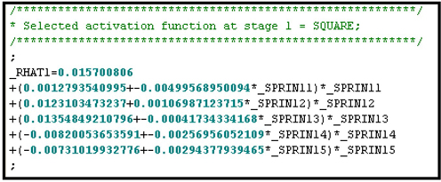
The model generated by the DMNeural Node is called an additive nonlinear model because it is the sum of the models generated at different stages of the training process. In other words, the output of the final model is the sum of the outputs of the models generated at different stages of the training process as shown in Display 5.80.

In the first stage a model is developed using the response variable is used as the target variable. An identity link is used if the target is interval scaled, and a logistic link function is used if the target is binary. The residuals of the model from the first stage are used as the target variable values in the second stage. The residuals of the model from the second stage are used as the target variable values in the third stage. The output of the final model is the sum of the outputs of the models generated in the first, second and third stages as can be seen in Display 5.80. The first, second and third stages of the model generation process are referred to as stage 0, stage 1 and stage 2 in the code shown in Displays 5.77 through 5.80. See SAS Enterprise Miner 12.1 Reference Help.

Display 5.76 shows the Properties panel of the DMNeural node used in this example.

Display 5.76

After running the DMNeural node, open the Results window and click Scoring→SAS code. Scroll down in the SAS Code window to view the SAS code, shown in Displays 5.77through 5.79.

Display 5.77 shows that the response variable is used as the target only in stage 0.

Display 5.77

The model at stage 1 is shown in Display 5.77. This code shows that the algorithm uses the residuals of the model from stage 0 (_RHAT1) as the new target variable.

Display 5.78

The model at stage 2 is shown in Display 5.79. In this stage, the algorithm uses the residuals of the model from stage 1 (_RHAT2) as the new target variable. This process of building the model in one stage from the residuals of the model from the previous stage can be called an additive stage-wise process.

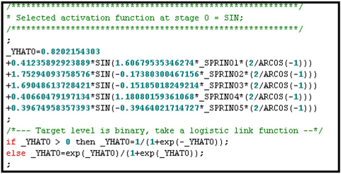
Display 5.79

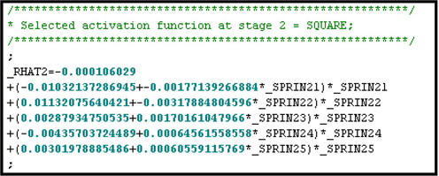
You can see in Display 5.79 that the Activation Function selected in stage 2 is SQUARE. The selection of the best activation function at each stage in the training process is based on the smallest SSE (Sum of Squared Error).

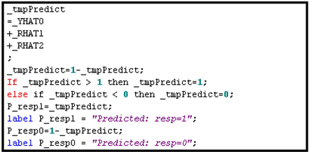
In Display 5.80, you can see that the final output of the model is the sum of the outputs of the models generated in stages 0, 1, and 2. Hence the underlying model can be described as an additive nonlinear model.

Display 5.80

5.10 Dmine Regression Node

The Dmine Regression node generates a Logistic Regression for a binary target. The estimation of the Logistic Regression proceeds in three steps.

In the first step, a preliminary selection is made, based on Minimum R-Square. For the original variables, the R-Square is calculated from a regression of the target on each input; for the binned variables, it is calculated from a one-way Analysis of Variance (ANOVA).

In the second step, a sequential forward selection process is used. This process starts by selecting the input variable that has the highest correlation coefficient with the target. A regression equation (model) is estimated with the selected input. At each successive step of the sequence, an additional input variable that provides the largest incremental contribution to the Model R-Square is added to the regression. If the lower bound for the incremental contribution to the Model R-Square is reached, the selection process stops.

The Dmine Regression node includes the original inputs and new categorical variables called AOV16 variables which are constructed by binning the original variables. These AOV16 variables are useful in taking account of the non-linear relationships between the inputs and the target variable.

After selecting the best inputs, the algorithm computes an estimated value (prediction) of the target variable for each observation in the training data set using the selected inputs.

In the third step, the algorithm estimates a logistic regression (in the case of a binary target) with a single input, namely the estimated value or prediction calculated in the first step.

Display 5.81 shows the Properties panel of the Dmine Regression node with default property settings.

Display 5.81

You should make sure that the Use AOV16 Variables property is set to Yes if you want to include them in the variable selection and model estimation.

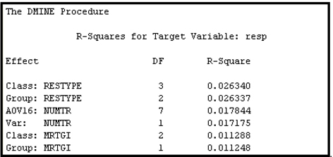
Display 5.82 shows the variable selected in the first step.

Display 5.82

Display 5.82 .

Display 5.83 shows the variables selected by the forward least-squares stepwise regression in the second step.

Display 5.83

5.11 Comparing the Models Generated by DMNeural, AutoNeural, and Dmine Regression Nodes

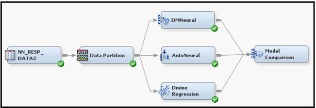
In order to compare the predictive performance of the models produced by the DMNeural, AutoNeural, and Dmine Regression nodes, I created the process flow diagram shown in Display 5.84.

Display 5.84

The results window of the Model Comparison node shows the Cumulative %Captured Response charts for the three models for the Training, Validation, and Test data sets.

Display 5.85 shows the Cumulative %Captured Response charges for the Training data set.

Display 5.85

Display 5.86 shows the Cumulative %Captured Response charges for the Validation data set.

Display 5.86

Display 5.87 shows the Cumulative %Captured Response charges for the Test data set.

Display 5.87

From the Cumulative %Captured Response, there does not seem to be a significant difference in the predictive performance of the three models compared.

5.12 Summary

• A neural network is essentially nothing more than a complex nonlinear function of the inputs. Dividing the network into different layers and different units within each layer makes it very flexible. A large number of nonlinear functions can be generated and fitted to the data by means of different architectural specifications.

• The combination and activation functions in the hidden layers and in the target layer are key elements of the architecture of a neural network.

• You specify the architecture by setting the Architecture property of the Neural Network node to User or to one of the built-in architecture specifications.

• When you set the Architecture property to User, you can specify different combinations of Hidden Layer Combination Functions, Hidden Layer Activation Functions, Target Layer Combination Functions, and Target Layer Activation Functions. These combinations produce a large number of potential neural network models.

• If you want to use a built-in architecture, set the Architecture property to one of the following values: GLM (generalized linear model, not discussed in this book), MLP (multilayer perceptron), ORBFEQ (Ordinary Radial Basis Function with Equal Widths and Heights), ORBFUN (Ordinary Radial Basis Function with Unequal Widths), NRBFEH (Normalized Radial Basis Function with Equal Heights and Unequal Widths), NRBFEV (Normalized Radial Basis Function with Equal Volumes), NRBFEW (Normalized Radial Basis Function with Equal Widths and Unequal Heights), NRBFEQ (Normalized Radial Basis Function with Equal Widths and Heights, and NRBFUN(Normalized Radial Basis Functions with Unequal Widths and Heights).

• Each built-in architecture comes with a specific Hidden Layer Combination Function and a specific Hidden Layer Activation Function.

• While the specification of the Hidden Layer Combination and Activation functions can be based on such criteria as model fit and model generalization, the selection of the Target Layer Activation Function should also be guided by theoretical considerations and the type of output you are interested in.

• In addition to the Neural Network node, three additional nodes, namely DMNeural, AutoNeural, and Dmine Regression nodes, were demonstrated. However, there is no significant difference in predictive performance of the models developed by these three nodes in the example used.

• The response and risk models developed here show you how to configure neural networks in such a way that they are consistent with economic and statistical theory, how to interpret the results correctly, and how to use the SAS data sets and tables created by the Neural Network node to generate customized reports.

5.13 Appendix to Chapter 5

Displays 5.88, 5.89, and 5.90 show the SAS code for calculating the lift for $L O S S F R Q$ .

Display 5.88

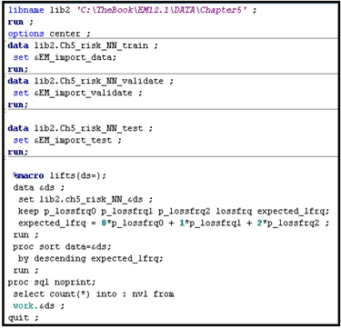
Display 5.89

Display 5.90

5.14 Exercises

1. Create a data source with the SAS data set Ch5_Exdata. Use the Advanced Metadata Advisor Options to create the metadata. Customize the metadata by setting the Class Levels Count Threshold property to 8. Set the Role of the variable EVENT to Target. On the Prior Probabilities tab of the Decision Configuration step, set Adjusted Prior to 0.052 for level 1 and 0.948 for level 0.

2. Partition the data such that 60% of the records are allocated for training, 30% for Validation, and 10% for Test.

3. Attach three Neural Network nodes and an Auto Neural node.
Set the Model Selection Criterion to Average Error in all the three Neural Network nodes.

a. In the first Neural Network node, set the Architecture property to Multilayer Perceptron and change the Target Layer Activation Function to Logistic. Set the Number of Hidden Units property to 5. Open the Optimization property and set the Maximum Iterations property to 100. Use default values for all other Network properties.

b. Open the Results window and examine the Cumulative Lift and Cumulative %Captured Response charts.

c. In the first Neural Network node, change the Target Layer Error Function property to Bernoulli, while keeping all other settings same as in (a).

d. Open the Results window and examine the Cumulative Lift and Cumulative %Captured Response charts. Did the model improved by changing the value of the Target Layer Error Function property to Bernoulli?

e. Open the Results window and the Score Code window by clicking File→Score→SAS Code. Verify that the formulas used in calculating the outputs of the hidden units and the estimated probabilities of the event are what you expected.

f. In the second Neural Network node, set the Architecture property to Ordinary Radial-Equal Width and the Number of Hidden Units property to 5. Use default values for all other Network properties.

g. In the third Neural Network node, set the Architecture Property to Normalized Radial-Equal Width. Set the Number of Hidden Units property to 5. Use default values for all other Network properties.

h. Set the AutoNeural node options as shown in Display 5.91.
Display 5.91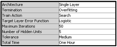

i. Use the default values for the properties of the Dmine Regression node.

Attach a Model Comparison node and run all models and compare the results. Which model is the best?

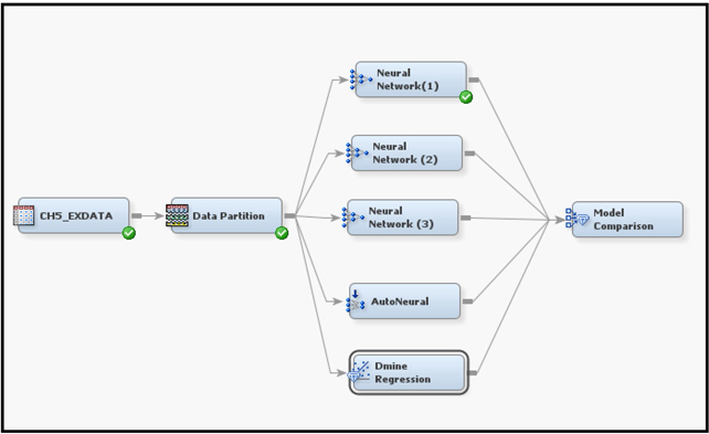
Display 5.92 shows the suggested process diagram for this exercise.

Display 5.92

Notes

1. Although the general discussion here considers two hidden layers, the two neural network models developed later in this book are based on a single hidden layer.

2. The terms observation, record, case, and person are used interchangeably.

3. Bishop, C.M. (1995) Neural Networks for Pattern Recognition. New York: Oxford University Press

4. Afifi, A.A and Clark, Virginia, Computer Aided Multivariate Analysis, CRC Press, 2004.

5. This is the target variable LOSSFRQ.

6. For the derivation of the error functions and the underlying probability distributions, see Bishop, C.M (1995) Neural Networks for Pattern Recognition, New York: Oxford University Press.

7. SAS Enterprise Miner uses the terms bin, percentile, and depth.

8. To transform an input to standardized units, the mean and standard deviation of the input across all records are computed, the mean is subtracted from the original input values, and the result is then divided by the standard deviation, for each individual record.

..................Content has been hidden....................

You can't read the all page of ebook, please click here login for view all page.

Table of Contents for Chapter 5: Neural Network Models to Predict Response and Risk

Create new playlist

Sign In

Sign Up

Chapter 5: Neural Network Models to Predict Response and Risk

5.1 Introduction

5.1.1 Target Variables for the Models

5.1.2 Neural Network Node Details

5.2 A General Example of a Neural Network Model

5.2.1 Input Layer

5.2.2 Hidden Layers

5.2.2.1 Hidden Layer 1: Unit 1

Hidden Layer 1: Unit 2

Hidden Layer 1: Unit 3

5.2.2.2 Hidden Layer 2

Hidden Layer 2: Unit 1

Hidden Layer 2: Unit 2

Hidden Layer 2: Unit 3

5.2.3 Output Layer or Target Layer

5.2.4 Activation Function of the Output Layer

5.3 Estimation of Weights in a Neural Network Model

5.4 A Neural Network Model to Predict Response

Input Data Node

Data Partition Node

5.4.1 Setting the Neural Network Node Properties

5.4.2 Assessing the Predictive Performance of the Estimated Model

5.4.3 Receiver Operating Characteristic (ROC) Charts

5.4.4 How Did the Neural Network Node Pick the Optimum Weights for This Model?

5.4.5 Scoring a Data Set Using the Neural Network Model

5.4.6 Score Code

5.5 A Neural Network Model to Predict Loss Frequency in Auto Insurance

5.5.1 Loss Frequency as an Ordinal Target

5.5.1.1 Target Layer Combination and Activation Functions

The first linear predictor for the ithith<math xmlns="http://www.w3.org/1998/Math/MathML"><mrow><msup><mi>i</mi><mrow><mi>t</mi><mi>h</mi></mrow></msup></mrow></math> customer/record is calculated as:

5.5.1.2 Target Layer Error Function Property

5.5.1.3 Model Selection Criterion Property

5.5.1.4 Score Ranks in the Results Window

5.5.2 Scoring a New Dataset with the Model

5.5.3 Classification of Risks for Rate Setting in Auto Insurance with Predicted Probabilities

5.6 Alternative Specifications of the Neural Networks

5.6.1 A Multilayer Perceptron (MLP) Neural Network

5.6.2 A Radial Basis Function (RBF) Neural Network

5.6.2.1 Radial Basis Function Neural Networks in the Neural Network Node

5.7 Comparison of Alternative Built-in Architectures of the Neural Network Node

5.7.1 Multilayer Perceptron (MLP) Network

5.7.2 Ordinary Radial Basis Function with Equal Heights and Widths (ORBFEQ)

5.7.3 Ordinary Radial Basis Function with Equal Heights and Unequal Widths (ORBFUN)

5.7.4 Normalized Radial Basis Function with Equal Widths and Heights (NRBFEQ)

5.7.5 Normalized Radial Basis Function with Equal Heights and Unequal Widths (NRBFEH)

5.7.6 Normalized Radial Basis Function with Equal Widths and Unequal Heights (NRBFEW)

5.7.7 Normalized Radial Basis Function with Equal Volumes (NRBFEV)

5.7.8 Normalized Radial Basis Function with Unequal Widths and Heights (NRBFUN)

5.7.9 User-Specified Architectures

5.7.9.1 Linear Combination Function with Different Activation Functions for the Hidden Layer

5.7.9.2 Default Activation Function with Different Combination Functions for the Hidden Layer

Add

Linear

EQSlopes

EQRadial

EHRadial

EWRadial

EVRadial

XRadial

5.7.9.3 List of Target Layer Combination Functions for the User-Defined Networks

5.7.9.4 List of Target Layer Activation Functions for the User-Defined Networks

5.8 AutoNeural Node

5.9 DMNeural Node

5.10 Dmine Regression Node

5.11 Comparing the Models Generated by DMNeural, AutoNeural, and Dmine Regression Nodes

5.12 Summary

5.13 Appendix to Chapter 5

5.14 Exercises

Notes

Table of Contents for
Chapter 5: Neural Network Models to Predict Response and Risk

The first linear predictor for the ith $i^{t h}$ customer/record is calculated as: