
Chapter 8: Customer Profitability
8.7 Alternative Scenarios of Response and Risk
8.9 Suggestions for Extending Results
8.1 Introduction
This chapter presents a general framework for calculating the profitability of different groups of customers, using a simplified example. The methodology can be extended to calculate profits at the individual customer level as well.
My goal is to illustrate how costs of acquisition and the costs associated with risk factors can affect the decision to acquire new customers, using the example of a credit card company.
For example, suppose you have a population of 10,000 prospects. A response model is used to score each of these 10,000 prospects. The prospects are arranged in descending order of the predicted probability of response and divided into deciles. A risk model is then used to calculate the risk rate for each prospect. In this simplified example, the risk rate is the probability of a customer defaulting on payment. Assume that a default results in a net loss of $10 for the credit card company on the average. If the customer does not default, the company makes $100. (These numbers are fictitious, and I use them for demonstration purposes only.) Table 8.1 shows the estimated response and risk rates for the deciles of the prospect population.
Table 8.1
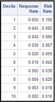
From Table 8.1, you can see that response rate and risk rate move in the same direction. The response rate is highest in the first decile and declines with succeeding higher-numbered deciles. A similar pattern is observed for the risk rate also. One reason why this may occur is that when a credit card company solicits applications for credit cards, the groups that respond most are likely to be those who cannot get credit elsewhere because of their relatively high risk rates.
In Table 8.1, the term risk rate is used in a general sense. A risk rate of 10% in decile 1 in Table 8.1 means that 10% of the persons who responded and are in decile 1 tend to default on their payments. (Here I am assuming that each person who responded is issued a credit card, but this assumption can be easily relaxed without violating the logic.) The response rate in a particular decile is the proportion of individuals in the decile who are responders. Display 8.1 graphs the response and risk rates for each decile.
Display 8.1
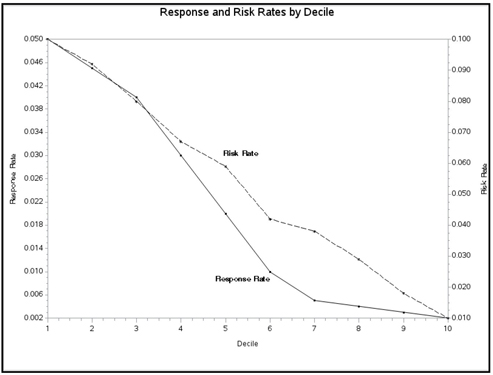
In Display 8.1, the horizontal axis shows the decile number. Decile 1 is the top decile, and decile 10 is the lowest decile.
Note: The example presented in this chapter is hypothetical and greatly simplified for the purpose of exposition; the costs and revenue figures are also quite arbitrary. The example refers to a credit card company but it can be extended to insurance and other companies as well. Details of the methodology should be modified according to the specific situation being analyzed. In many situations, for example, customers with a high response rate to a direct mailing campaign might also pose higher risks to the company that is soliciting business.
8.2 Acquisition Cost
New customers are acquired through channels such as newspaper or Internet advertisements, radio and TV broadcasting, direct mail, etc. If a company spends dollars on a particular channel, and as a result it acquires customers, then the average cost of acquisition per customer is . For direct mail, this can be calculated easily. Suppose the response rate is in a segment of the target population and suppose the cost of sending one mail piece is dollars. If mail is sent to N customers from that segment, then the average cost of acquiring a customer is
This means that as the response rate decreases, the average acquisition cost increases. Display 8.2 illustrates this relationship.
Display 8.2

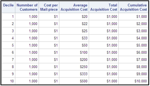
Table 8.2 shows the acquisition cost by decile. Since the response rate declines with succeeding higher-numbered deciles, the average acquisition cost increases. When the company sends mail to the 1,000 prospects in the top decile (decile 1) inviting them to purchase a product, at a cost of $1 per piece of mail, the total cost is $1,000. In return, the company acquires 50 customers, as the response rate in the top decile is 0.05. The average cost of acquisition is therefore $1,000/50 = $20. Similarly, the average cost of acquisition for the second decile is $1,000/45 = $22.22. The last column shows the cumulative acquisition cost. If all the prospects in the top two deciles are sent a mail piece, the total cost would be $2,000. This is the cumulative acquisition cost, and it is an important item in determining the optimum cut-off point for mailing.
Table 8.2
8.3 Cost of Default
If a customer defaults on payment, his credit card company incurs a loss. The credit card company might face other types of risk, but for the purpose of illustration, only one type of risk, the risk of default, is considered here.
Table 8.3 illustrates the costs due to the risk of default. Assume, for the purpose of illustration, that each event (default) results in a cost of $10 to the credit card company. In general, you can include more events with associated probabilities and with more realistic costs in these calculations.
In this simplified example, the top decile has 50 responders. Of these responders, five people (the risk rate is 0.1) tend to default on their payments, resulting in an expected loss of $50 to the company. In the second decile there are 45 responders (since the response rate is 4.5%). Of these 45 customers, 9.2% are likely to default on their payments, resulting in an expected loss of 45 × 0.092 × $10 = $41. If the company targets the top two deciles, it will experience an expected loss of $91. This is the cumulative loss1 for the second decile. Similarly cumulative losses can be calculated for the remaining deciles.
Table 8.3

8.4 Revenue
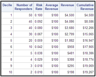
Revenue depends on the number of customers who do not default. These revenues are shown in Table 8.4. To simplify the example, I have assumed that a customer who defaults on payment generates no revenue. This assumption can easily be relaxed without violating the logic of my argument.
In the top decile, there are 50 responders, but only 45 of them are customers in good standing at the end of the year (assuming that our analysis is based on calculations for one year). Hence the revenue generated in the top decile is 45 × $100 = $4,500. A similar calculation yields revenue of $4,086 for the second decile. Hence the cumulative revenue for the first two deciles is $8,586. Similarly, cumulative revenue calculated for all the remaining deciles is shown in Table 8.4.
Table 8.4
8.5 Profit
If, for example, the company targets the top two deciles, the expected revenue will be $8,586, the expected acquisition cost will be $2,000, and the expected losses will be $91. Therefore, the expected cumulative profit will be $8,586 – $2,000 – $91 = $6,495. Table 8.5 shows the cumulative profit for all the deciles.
Table 8.5

The optimum cut-off point is where the cumulative profit peaks. In our example, it occurs at decile 5. The company can maximize its profit by sending mail to only the 5,000 prospects who are in the top five deciles. This can be seen from Display 8.3.
Display 8.3
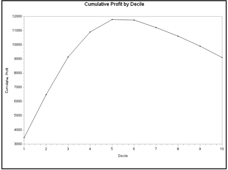
The cumulative profit peaks at the fifth decile because, beyond the fifth decile, the marginal profit earned by mailing to an additional decile is negative.
The marginal cost at the fifth decile is defined as the additional cost that the company would incur in acquiring the responders in the next (sixth) decile. The marginal revenue at the fifth decile is defined as the additional revenue the company would earn if it acquired all the responders in the next (sixth) decile. The marginal profit at the fifth decile is defined as the additional profit the company would make if it acquired the responders in the next (sixth) decile, which is the marginal revenue minus the marginal cost.
Beyond the fifth decile, the marginal cost outweighs the marginal revenue. Hence the marginal profit is negative. This is depicted in Display 8.4.
Display 8.4

8.6 The Optimum Cut-off Point
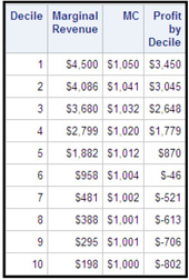
The optimization problem can be analyzed in terms of marginal revenue and marginal cost. In this simplified example, marginal revenue (MR) at any decile is the additional revenue that is gained by mailing to the next decile, in addition to the previous deciles. Similarly, the marginal cost (MC) at any decile is the additional cost the company incurs by adding an additional decile for mailing. The marginal cost and marginal revenue, which are derived from the figures in Table 8.5, are shown in Table 8.6. In Table 8.5, you can see that if the company mails to the top five deciles, the cumulative (total) revenue is $16,947 and cumulative (total) cost is $5,155. If the company wants to mail to the top six deciles, the revenue will be $17,905 and cost will be $6,160. Hence the marginal revenue at 5 is $17,905 – $16,947 = $958 and marginal cost is $6,160 – $5,155 = $1005. Since marginal cost exceeds marginal revenue, the cumulative profits will decline by adding the sixth decile to the mailing. The marginal revenues and marginal costs at different deciles shown in Table 8.6 are plotted in Display 8.5.
Table 8.6
Display 8.5
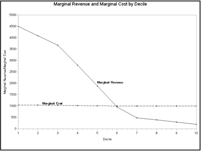
Display 8.5 shows that the point at which MR=MC is somewhere between the fifth and sixth deciles. As an approximation, you can stop mailing after the fifth decile.
In the above example, the profits are calculated for one year only for the sake of simplicity. Alternatively, you can calculate profits over a longer period of time or add other complications to the analysis to make it more pertinent to the business problem you are trying to solve. All these calculations can be made in the SAS Code node.
8.7 Alternative Scenarios of Response and Risk
In the example presented in Table 8.1, it is assumed that response rate and risk rate move in the same direction. The response rate is highest in the first decile, and declines with succeeding higher-numbered deciles. A similar pattern is observed for the risk rate. However, there are many situations in which response rate and risk rate may not show this type of a pattern. In such situations, you can estimate two scores for each customer—one based on probability of response, and the other based on risk. Next, the prospects can be arranged in a 10x10 matrix, each cell of the matrix consisting of the number of customers belonging to the same response-decile and risk-decile. Acquisition cost, cost of risk, revenue, and profit can be calculated for each cell, and acquisition decisions can be made for each group of customers based on the profitability of the cells.
8.8 Customer Lifetime Value
At the end of Section 8.6, I pointed out that the analysis of customer acquisition based on the marginal profit from mailing to additional prospects could be performed with a more distant horizon than the one year analysis shown in my example. Taking this to its logical conclusion, calculations of profitability at the level of an individual customer can be extended further by calculating the customer’s lifetime value. For this you need answers to three questions:
• What is the expected residual lifetime of each customer?
• What is the flow of revenue that the customer is expected to generate in his “lifetime”?
• What are the future costs to the company of acquiring and retaining each customer?
Proper analysis of these elements can yield valuable insights into the type of actions that a company can take for extending the residual lifetime, the customer lifetime value, or both.
8.9 Suggestions for Extending Results
In the analysis presented in this chapter, Revenue, Cost, and Profit are calculated for each decile. Alternatively, you can do the same calculations for each percentile in your data base of prospects, rather than for each decile. This would enable you to choose the cutoff point for a mailing or other marketing promotion with greater precision. In addition, in my example, only one type of risk is identified. If, however, there is more than one type of risk, you can model competing risks by means of logistic hazard functions using either the Regression node or the Neural Network node of SAS Enterprise Miner.
Note
1. The losses are calculated using the estimated probabilities, and hence, strictly speaking, they should be called expected losses. But here I use the terms losses and expected losses interchangeably.