Chapter 9: Introduction to Predictive Modeling with Textual Data

9.1 Introduction

9.1.1 Quantifying Textual Data: A Simplified Example

9.1.2 Dimension Reduction and Latent Semantic Indexing

9.1.3 Summary of the Steps in Quantifying Textual Information

9.2 Retrieving Documents from the World Wide Web

9.2.1 The %TMFILTER Macro

9.3 Creating a SAS Data Set from Text Files

9.4 The Text Import Node

9.5 Creating a Data Source for Text Mining

9.6 Text Parsing Node

9.7 Text Filter Node

9.7.1 Frequency Weighting

9.7.2 Term Weighting

9.7.3 Adjusted Frequencies

9.7.4 Frequency Weighting Methods

9.7.5 Term Weighting Methods

9.8 Text Topic Node

9.8.1 Developing a Predictive Equation Using the Output Data Set Created by the Text Topic Node

9.9 Text Cluster Node

9.9.1 Hierarchical Clustering

9.9.2 Expectation-Maximization (EM) Clustering

9.9.3 Using the Text Cluster Node

9.10 Exercises

9.1 Introduction

This chapter shows how you can use SAS Enterprise Miner’s text mining nodes¹ to quantify unstructured textual data and create data matrices and SAS data sets that can be used for statistical analysis and predictive modeling. Some examples of textual data are: web pages, news articles, research papers, insurance reports, etc. In text mining, each web page, news article, research paper, etc. is called a document. A collection of documents, called a corpus of documents, is required for developing predictive models or classifiers. Each document is originally represented by a string of characters. In order to build predictive models from this data, you need to represent each document by a numeric vector whose elements are frequencies or some other measure of occurrence of different terms in the document. Quantifying textual information is nothing but converting the string of characters in a document to a numerical vector of frequencies of occurrences of different words or terms. The numerical vector is usually a column in the term-document matrix, whose columns represent the documents. A data matrix is the transpose of the term-document matrix. You can attach a target column with known class labels of the documents to the data matrix. Examples of class labels are: Automobile Related, Health Related, etc. You need a data matrix with a target variable for developing predictive models. This chapter shows how you can use the SAS Enterprise Miner’s text miner nodes to help create a data matrix, reduce its dimensions in order to create a compact version of the data matrix, and include it in a SAS data set which can be used for statistical analysis and predictive modeling.

In order to better understand the purpose of quantifying textual data, let us take an example from marketing. Suppose an automobile seller (advertiser) wants to know if a visitor to the Web is intending to buy an automobile in the near future. A person who intends to buy an automobile in the near future can be called an “auto intender”. In order to determine whether a visitor to the Web is an auto intender or not, the auto seller needs to determine if the pages the visitor views frequently are auto related. The auto seller can use a predictive model that can help him decide if a web page is auto related. Logistic regressions, neural networks, decision trees, and support vector machines can be used for assigning class labels such as Auto Related and Not Auto Related to the web pages and other documents.

9.1.1 Quantifying Textual Data: A Simplified Example

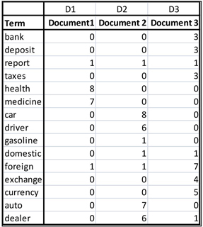
The need for quantifying textual data also arises in query processing by search engines. Suppose you send the query “Car dealers” to a search engine. The search engine compares your query with a collection of documents with pre-assigned labels. For illustration, suppose there are only three documents in the collection (in the real world there may be thousands of documents) where each document is represented by a vector of terms as shown in Table 9.1

Table 9.1

9.1.1.1 Term-Document Matrix

The rows in a term-document matrix represent the occurrence (some measure of frequency) of a term in the documents represented by the columns. The table shown in Display 9.1 is an example of a term-document matrix.

In Table 9.1, Document1 is represented by column D1, Document2 by column2, and Document3 by column 3. There are 15 terms and 3 documents. So the term-document matrix is 15x3, and the document-term matrix, which is the transpose of the term-document matrix, is 3X15. In order to compare the query with each document, we need to represent the query as a vector consistent with the document vectors.

The query is converted to the row vector $q^{\prime }=(00000\text{ 0 }100000001)$, where 1 indicates the occurrence of a term in the query and 0 indicates the non-occurrence. In the query vector $q$ the 7^th and 15^th elements are equal to 1, and all other elements are equal to 0 since the 7^th and 15^th elements of the term vector are “car” and “dealer”. The term vector is the first column in Table 9.1 and we can write it in vector notation as $T^{\prime }$ = (bank, deposit, report, taxes, health, medicine, car, driver, gasoline, domestic, foreign, exchange, currency, auto, dealer).

In order to facilitate the explanations, let us represent the documents by the following vectors:

$D{1}^{\prime }=\left(\text{0 0 1 0 8 7 0 0 0 0 1 0 0 0 0}\right)$ , $D{2}^{\prime }=\left(\text{0 0 1 0 0 0 8 6 1 1 1 0 0 7 6}\right)$ and $D{3}^{\prime }=\left(\text{3 3 1 3 0 0 0 0 0 1 7 4 5 0 1}\right)$.

In order to determine which document is closest to the query, we need to calculate the scores of each document vector with the query. The score of a document can be calculated as the inner product of the query vector and the document vector.

The score for Document 1 is: $D{1}^{\prime }q$ = 0

The score for Document 2 is $D{2}^{\prime }q$ = 14

The score for Document 3 is: $D{3}^{\prime }q$ = 1

9.1.1.2 Boolean Retrieval

The above calculations show how a query can be processed or information is retrieved from a collection of documents. An alternative way of processing queries is the Boolean Retrieval method. In this method, the occurrence of a word is represented by 1, and the non-occurrence of a word is represented by 0.

$D{1}^{\prime }=\left(\text{0 0 1 0 1 1 0 0 0 0 1 0 0 0 0}\right)$, $D{2}^{\prime }=\left(\text{0 0 1 0 0 0 1 1 1 1 1 0 0 1 1}\right)$ and $D{3}^{\prime }=\left(\text{1 1 1 1 0 0 0 0 0 1 1 1 1 0 1}\right)$.

The query is represented by a vector whose components are the frequencies of the occurrences of various words. Suppose the query consists of four occurrences of the word “car” and three occurrences of the word “dealer.” Then the query can be represented by the vector:

 

$$q^{\prime }=(00000\text{ 0 }400000003)$$

The score for Document 1 is: $D{1}^{\prime }q$ = 0

The score for Document 2 is $D{2}^{\prime }q$ = 7

The score for Document 3 is: $D{3}^{\prime }q$ = 3.

Since the score is the highest for Document2, the person who submitted the query should be directed to Document2, which contains information on auto dealers.

9.1.1.3 Document-Term Matrix and the Data Matrix

A document-term matrix is the transpose of the term-document matrix, such as the one shown in Display 9.1. A data matrix is same as the document-term matrix. The data matrix can be augmented by an additional column that shows the labels given to the documents.

In the illustration given above, the columns of the term-document matrix are the vectors $D1$, $D2$ and $D3$. The rows of the document-term or the data matrix are same as the columns of the term-document matrix.

You can verify that the vectors $D1,D2\text{ and D}3$ are the second, third and fourth columns in Table 9.1. From Table 9.1, we can define the data matrix as:

 

$$D=\left[\begin{array}{l}\text{0 0 1 0 8 7 0 0 0 0 1 0 0 0 0}\\ \text{0 0 1 0 0 0 8 6 1 1 1 0 0 7 6}\\ \text{3 3 1 3 0 0 0 0 0 1 7 4 5 0 1 }\end{array}\right](9.1)$$

The data matrix has one row for each document and one column for each term. Therefore, in this example, its dimension is 3x15. In a SAS data set, this data matrix has 3 rows and 15 columns or 3 observations and 15 variables, where each variable is a term.

If you already know the labels of the documents, you can add an additional column with the labels. For example if we give the label 1 to a document in which the main subject is automobiles and give the label 0 if the main subject of the document is not automobiles. Then the augmented data matrix with an additional column of labels can be used to estimate a logistic regression, which can be used to classify a new document as Auto Related or Not Auto Related.

In the example presented above, the elements of the data matrix are frequencies of occurrences of the terms in the documents. The value of the $i{j}^{th}$ element of $D$ is the frequency of $j^{th}$ term in the $i^{th}$ document. From the $D$ matrix shown above in Equation 9.1, you can see that the word “health” appears 8 times in Document1.

In practice, adjusted frequencies rather than the raw frequencies are used in a D matrix. The adjusted frequency can be calculated as $tfidf(i,j)=tf(i,j)*\log \left(\frac{N}{df(j)}\right)$ , where $tf(i,j)$ = frequency of $j^{th}$ term in $i^{th}$ document (same as $f_{ij}$), $df(j)$ =document frequency (number of documents containing the $j^{th}$ term) and $N$ = Number of documents. $tfidf(i,j)$ is a measure of the relative importance of the $j^{th}$ term in the $i^{th}$ document. We refer to $tfidf(i,j)$ as the adjusted frequency. There are other measures of relative importance of terms in a document.

In the examples presented in this and the next section, raw frequencies ($f_{ij}$) are used for illustrating the methods of quantification and dimension reduction.

The main tasks of the quantifying textual data are:

 

1. Constructing the term-document matrix from a collection of documents where the elements of the matrix are the frequency of occurrence of the words in each document. The elements of the term-document matrix can be $tfidf$ as described above, or some other measure. The term-document matrix can be of a very large size such as 500,000x1,000,000 representing 500,000 terms and 1,000,000 documents. The corresponding data matrix has 1,000,000 rows (documents) and 500,000 columns (terms).
Singular Value Decomposition (SVD) is applied to derive a smaller matrix such as 100x1,000,000, where the rows of the new matrix are called SVD dimensions. These dimensions may be related to meaningful concepts.

After applying the SVD, the data matrix has 1,000,000 rows and 100 columns. The rows are documents (observations) and the columns are SVD dimensions.

The above tasks can be performed by various text mining nodes as described in this chapter.

9.1.2 Dimension Reduction and Latent Semantic Indexing

In contrast to the data matrix used in this example, the real-life data matrices are very large with thousands of documents and tens of thousands of terms. Also, these large data matrices tend to be sparse. Singular Value Decomposition (SVD), which is demonstrated in this section, is used to create smaller and denser matrices from large sparse data matrices by replacing the terms with concepts or topics. The process of creating concepts or topics from the terms is demonstrated in this section. The data matrix with concepts or terms in the columns is much smaller than the original data matrix. In this example, the D matrix (shown earlier in this chapter) which is 3x15 is replaced by a 3x3 data matrix $D^{*}$. The rows of $D^{*}$ are documents, and the columns contain concepts or topics.

Singular Value Decomposition² factors the term-document matrix into three matrices in the following way:

 

$$A=U\mathrm{\Sigma }{V}^{\prime }\text{, where }A\text{ is a }m\times n\mathrm{term}-\mathrm{document}\mathrm{matrix}(9.2)$$

$m$ = number of terms and $n$ = number of documents

$U$ is an $m\times k$ term-concept matrix, where $k\le r=rank(A)$. The columns of $U$ are eigenvectors of $A{A}^{\prime }$ and they are called the Left Singular Vectors. In this example $k=3.$

$\mathrm{\Sigma }$ is a diagonal matrix of size $k\times k$. The diagonal elements of $\mathrm{\Sigma }$ are singular values which are the square roots of the nonzero eigenvalues of both $A{A}^{\prime }\text{ and }{A}^{\prime }A$. The singular values in the diagonal elements of $\mathrm{\Sigma }$ are arranged in a decreasing order (as shown in the example below).

$V$ is a concept-document matrix of size $n\times k$. The columns of $V$ are eigenvectors of $A^{\prime }A$ and they are called the Right Singular Vectors.

Applying Equation 9.2 to the term-document matrix shown in Table 9.1, we get:

$$\begin{array}{l}A=\left[\begin{array}{rrr}\hfill 0& \hfill 0& \hfill 3\\ \hfill 0& \hfill 0& \hfill 3\\ \hfill 1& \hfill 1& \hfill 1\\ \hfill 0& \hfill 0& \hfill 3\\ \hfill 8& \hfill 0& \hfill 0\\ \hfill 7& \hfill 0& \hfill 0\\ \hfill 0& \hfill 8& \hfill 0\\ \hfill 0& \hfill 6& \hfill 0\\ \hfill 0& \hfill 1& \hfill 0\\ \hfill 0& \hfill 1& \hfill 1\\ \hfill 1& \hfill 1& \hfill 7\\ \hfill 0& \hfill 0& \hfill 4\\ \hfill 0& \hfill 0& \hfill 5\\ \hfill 0& \hfill 7& \hfill 0\\ \hfill 0& \hfill 6& \hfill 1\end{array}\right],U=\left[\begin{array}{rrr}\hfill -0.04498& \hfill -0.19748& \hfill -0.18727\\ \hfill -0.04498& \hfill -0.19748& \hfill -0.18727\\ \hfill -0.08883& \hfill -0.10807& \hfill 0.01974\\ \hfill -0.04498& \hfill -0.19748& \hfill -0.18727\\ \hfill -0.02700& \hfill -0.47266& \hfill 0.57880\\ \hfill -0.02363& \hfill -0.41358& \hfill 0.50645\\ \hfill -0.56366& \hfill 0.13471& \hfill 0.07855\\ \hfill -0.42275& \hfill 0.10103& \hfill 0.05891\\ \hfill -0.07046& \hfill 0.01684& \hfill 0.00982\\ \hfill -0.08545& \hfill -0.04899& \hfill -0.05261\\ \hfill -0.17879& \hfill -0.50303& \hfill -0.35481\\ \hfill -0.05998& \hfill -0.26331& \hfill -0.24970\\ \hfill -0.07497& \hfill -0.32914& \hfill -0.31212\\ \hfill -0.49321& \hfill 0.11787& \hfill 0.06873\\ \hfill -0.43774& \hfill 0.03520& \hfill -0.00351\end{array}\right]\text{, }\mathrm{\Sigma }\text{=}\left[\begin{array}{rrr}\hfill 13.86679& \hfill 0.00000& \hfill 0.00000\\ \hfill 0.00000& \hfill 11.10600& \hfill 0.00000\\ \hfill 0.00000& \hfill 0.00000& \hfill 10.41004\end{array}\right]\text{ and}\\ \\ V=\left[\begin{array}{rrr}\hfill -0.04680& \hfill -0.65617& \hfill 0.75316\\ \hfill -0.97703& \hfill 0.18701& \hfill 0.10221\\ \hfill -0.20792& \hfill -0.73108& \hfill -0.64985\end{array}\right]\end{array}$$

Table 9.2 shows the columns of the term-concept matrix U.

Table 9.2

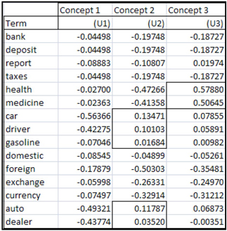
The columns in table 9.2 can be considered as weights of different terms into various concepts. These weights are analogous to factor loadings in Factor Analysis. If we consider that the vectors U1, U2, and U3 represent different concepts, we will be able to label these concepts based on the weights.

Since the terms “health” and “medicine” have higher weights than other terms in column U3, we may be able to label U3 to represent the concept “health”. Since the terms “car,” “driver,” “gasoline,” “auto,” and “dealer” have higher weight than other terms in U2, we may be able to label column U2 to represent the concept “auto related”. Labeling is not so clear in the case for column U1, but if you compare the weights of the term across different documents, you may get some clues for labeling U1 also. The weight of “bank” in column U1 is higher than in columns U2 and U3. Similarly the terms “deposit,” “taxes,” “exchange,” and “currency” have higher weights in column U1 than in other columns. So we may label column U1 as Economics or Finance.

The columns of the matrix $U$ can be considered as points in an $m$-dimensional space ($m$ =15 in our example). The values in the columns are the coordinates of the points. By representing the points in a different coordinate system, you may be able to identify the concepts more clearly. Representing the points in a different coordinate system is called rotation. To calculate the coordinates of a point represented by a column in the U, you multiply it by a rotation matrix. For example, let the first column of the matrix U be U1. U1 is a point in 15-dimenstional space. To represent this point (U1) in a different coordinate system, you multiply U1 by a rotation matrix R. This multiplication gives new coordinates for the point represented by vector U1. By using the same ration matrix R, new coordinates can be calculated for all the columns of the term-concept matrix U. These new coordinates may show the concepts more clearly.

No rotation is performed in our example, because we were able to identify the concepts from the U matrix directly. In SAS Text Miner the Text Topic node does rotate the matrices generated by the Singular Value Decomposition. In other words, the Text Topic node performs a rotated Singular Value Decomposition.

9.1.2.1 Reducing the Number of Columns in the Data Matrix

Making use of the columns of the U matrix as weights and applying them to the rows of the data matrix D shown in Equation 9.1, we can create a data matrix with fewer columns in the following way. In general the number of columns selected in the $U$ matrix = $k<r=rank(A).$ In our example,$k=3$, as stated previously.

 

$$D^{*}=D\times U\times {\mathrm{\Sigma }}^{-1}(9.3)$$

The original data matrix D has 3 rows and 15 columns, each column representing a term. The new data matrix $D^{*}$ has the same number of rows but only 3 columns.

In our example:

 

$$D*=\left[\begin{array}{rrr}\hfill -0.04680& \hfill -0.65617& \hfill -0.75316\\ \hfill -0.97703& \hfill 0.18701& \hfill -0.10221\\ \hfill -0.20792& \hfill -0.73108& \hfill 0.64985\end{array}\right](9.4)$$

The new data matrix has 3 rows and 3 columns.

The original data matrix and reduced data matrix is shown in Tables 9.3 and 9.4.

Table 9.3

The data matrix with reduced dimensions appended by a target column is shown in Table 9.4.

Table 9.4

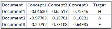
The variables Concept1, Concept2, and Concept 3 for the three documents in the data set shown in Table 9.4 are calculated using the Equation 9.3 and shown in a matrix form in Equation 9.4. I leave it to you to carry out the matrix multiplications shown in Equation 9.3 and arrive at the compressed data matrix shown in Equation 9.4 and hence the values of Concept1, Concept2, and Concept 3 shown in Table 9.4. The variables Concept1, Concept2, and Concept3 shown in Table 9.4 can also be called svd_1, svd_2, and svd_3.

I have added an additional column named Target with known labels of the documents. The label H stands for Health Related, A stands for Auto Related, and E stands for Economics Related.

You can use a data set that looks like Table 9.4 and create a binary target that takes the value if the document is Auto Related and 0 if it is Not Auto Related. You can use such a table for estimating a logistic regression that you can use to predict whether a document is Auto Related or Not Auto Related.

Using Singular Value Decomposition (SVD) to identify patterns in the relationships between the terms and concepts, as we did above, is called Latent Semantic Indexing.

The starting point for the calculation of the Singular Value Decomposition is the term-document matrix such as the one shown in Table 9.1.

9.1.3 Summary of the Steps in Quantifying Textual Information

1. Retrieve the documents from the internet or from a directory on your computer and create a SAS data set. In this data set, the rows represent the documents and the columns contain the text content of the document. Use the %TMFILTER macro or the Text Import node.

2. Create terms. Break the stream of characters of the documents³ into tokens by removing all punctuation marks, reducing words to their stems or roots,⁴ and removing stop words (articles) such as a, an, the, at, in, etc. Use the Text Parsing node to do these tasks.

3. Reduce the number of terms. Remove redundant or unnecessary terms by using the Text Filter node

4. Create a term-document matrix⁵ with rows that correspond to terms, columns that correspond to documents (web pages, for example), and whose entities are the adjusted frequencies of occurrences of the terms.
Create a smaller data matrix by performing a Singular Value Decomposition of the term-document matrix

In the following sections, I show how these steps are implemented in SAS text mining nodes. I use the Federalist Papers to demonstrate this process.

9.2 Retrieving Documents from the World Wide Web

You can retrieve documents from the World Wide Web and create SAS data sets from them using the %TMFILTER macro or the Text Import node, which is used only in a client-server environment.

9.2.1 The %TMFILTER Macro

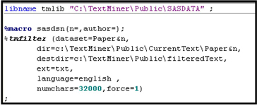
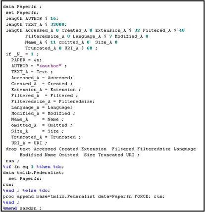
You can retrieve documents from web sites using the %TMFILTER macro, as shown in Display 9.1.

Display 9.1

The code segment shown in Display 9.1 retrieves Paper 1 of the Federalist Papers from the URL http://www.constitution.org/fed/federa01.htm. When I ran the above macro, six HTML files were created and stored in the directory C:TextMinerPublic mfdir. The file called file1.html contains Federalist Paper 1. A partial view of this paper is shown in Display 9.2.

Display 9.2

The directory c:TextMinerPublic mfdir_filtered contains text files with the same content as the HTML files. A partial view of the text file created is shown in Display 9.3.

Display 9.3

From the output shown in Display 9.4, you can see that six files were imported and that none of them were truncated.

Display 9.4

In addition, a SAS data set named TEXT is created and stored in the directory C:TextMinerPublicSASDATA. This data set has six rows, each row representing a file that is imported. The first row is relevant to us, since it has Federalist Paper 1. All other files represent other information about the web site itself. Since we are interested in analyzing the Federalist Papers, we can retain only the first row. The data set consists of a variable named Text, which contains the text content of the entire Paper 1.

If you call the macro (shown in Display 9.1) 85 times using a %DO loop and append the SAS data sets created at each iteration , you get a SAS data set with 85 rows, each row representing a document. In this example, each document is a Federalist Paper.

9.3 Creating a SAS Data Set from Text Files

If the text files are previously retrieved and stored in a directory, you can create SAS data sets from them directly. Display 9.5 shows how to create SAS data sets from text files stored in the directory C:TextMinerPublicCurrentTextPaper&n, where &n = 1, 2, …, 85.

Display 9.5

The arguments in the %TMFILTER macro are:

dataset	=	name of the output data set.
dir	=	path to the directory that contains the documents to process.
destdir	=	path to specify the output in the plain text format.
ext	=	extension of the files to be processed.
numchars	=	length of the text variable in the output data set.
force	= 1	keeps the macro from terminating if the directory specified in destdir is not empty.

Display 9.5 (cont’d)

Using the program shown in Display 9.6, I renamed the variables and also created the target variable.

Display 9.6

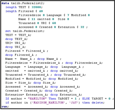
The %TMFILTER macro can create SAS data sets from Microsoft Word, Microsoft Excel, Adobe Acrobat, and several other types of files.

Display 9.7 shows the contents of the SAS data created by the program shown in Display 9.6.

Display 9.7

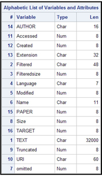
In the data set, there is one row per document. The variable PAPER identifies the document, and the variable TEXT contains the entire text content of the document.

9.4 The Text Import Node

The Text Import Node is an interface to the %TMFILTER macro described above.

You can use the Text Import node to retrieve files from the Web or from a server directory, and create data sets that can be used by other text mining nodes. The Text Import node relies on the SAS Document Conversion Server installed and running on a Windows machine. The machine must be accessible from the SAS Enterprise Miner Server via the host name and port number that were specified at the install time.

If you are not set up in a client-server mode, you can use the %TMFILTER macro as demonstrated in Section 9.2.1.

9.5 Creating a Data Source for Text Mining

Since the steps involved in creating a data source are the same as those demonstrated in Chapter 2, they are not shown here. Display 9.8 shows the variables in the data source.

Display 9.8

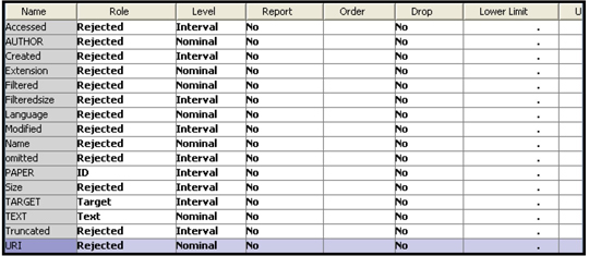
The roles of the variables TARGET, TEXT, and PAPER are set to Target, Text, and ID respectively. I set the roles of all other variables to Rejected as I do not use them in this chapter.

The variable TARGET takes the value 1 if the author of the paper is Hamilton and 0 otherwise, as defined by the SAS code shown in Display 9.6. The variable TEXT is the entire text of a paper.

9.6 Text Parsing Node

Text parsing is the first step in quantifying textual data contained in a collection of documents.

The Text Parsing node tokenizes the text contained in the documents by removing all punctuation marks. The character strings without spaces are called tokens, words or terms. The Text Parsing node also does stemming by replacing the words by their base or root. For example, the words “is” and “are” are replaced by the word “be”. The Text Parsing node also removes stop words, which consist of mostly articles and prepositions. Some examples of stop words are: a, an, the, on, in, above, actually, after, and again.

Display 9.9 shows a flow diagram with the Text Parsing node.

Display 9.9

Display 9.10 shows the variables processed by the Text Parsing node.

Display 9.10

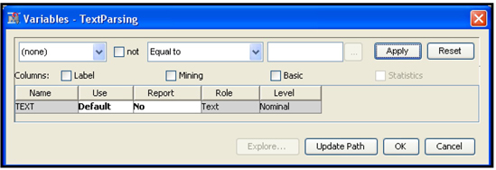
The Text Parsing node processes the variable TEXT included in the analysis and collects the terms from all the documents.

Display 9.11 shows the properties of the Text Parsing node.

Display 9.11

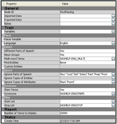
You can also provide a start list and stop list of terms. The terms in the start list are included in the collection of terms, and the terms in the stop list are excluded. You can open SAS Enterprise Miner: Reference Help to find more details about the properties.

After running the Text Parsing node, open the Results to see a number of graphs and a table that shows the terms collected from the documents and their frequencies in the document collection. Display 9.12 shows the ZIPF plot.

Display 9.12

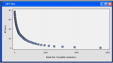
The horizontal axis of the ZIPF plot in Display 9.12 shows the terms by their rank and the vertical axis shows the number of documents in which the term appears. Display 9.13 gives a partial view of the rank of each term and the number of documents where the term appears.

Display 9.13

To see term frequencies by document, you need the two data sets &EM_LIB..TEXTPARSING_TERMS and &EM_LIB..TEXTPARSING_TMOUT, where &EM_LIB refers to the directory where these data sets are stored. You can access these data sets via the SAS Code node.

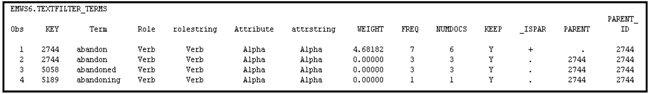
Table 9.5 shows selected observations from the data set &EM_LIB..TEXTPARSING_TERMS.

Table 9.5

Table 9.6 shows the distinct values of the terms.

Table 9.6

Table 9.7 shows the selected observations from &EM_LIB..TEXTPARSING_TMOUT.

Table 9.7

Table 9.8 shows a join of Tables 9.6 and 9.7.

Table 9.8

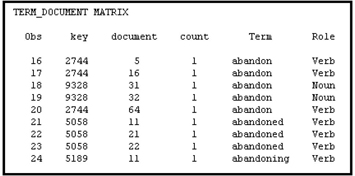
You can arrange the data shown in Table 9.8 into a term-document matrix. When the term “abandon” is used as a verb, it is given the key 2744, and when it is used as a noun it is given the key 9328.

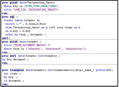
Displays 9.14A and 9.14B show the SAS code that you can use to generate Tables 9.5 – 9.8. Display 9.14B shows how to create a term-document matrix using PROC TRANSPOSE. The term-document matrix shows raw frequencies of the terms by document.

Display 9.14A

Display 9.14B

9.7 Text Filter Node

The Text Filter node reduces the number of terms by eliminating unwanted terms and filtering documents using a search query or a where clause. It also adjusts the raw frequencies of terms by applying term weights and frequency weights.

9.7.1 Frequency Weighting

If the frequency of $i^{th}$ term in the $j^{th}$ document is $f_{ij}$, then you can transform the raw frequencies using a formula such as $g\left(f_{ij}\right)={\log }_2\left(f_{ij}+1\right)$. Applying transformations to the raw frequencies is called frequency weighting since the transformation implies an implicit weighting. The function $g\left(f_{ij}\right)$ is called the fFquency Weighting Function. The weight calculated using the Frequency Weighting Function is called frequency weight.

9.7.2 Term Weighting

Suppose you want to give greater weight to terms that occur infrequently in the document collection. You can apply a weight that is inversely related to the proportion of documents that contain the term. If the proportion of documents that contain the term $t_i=P\left(t_i\right)$ , then the weight applied is $w_i={\log }_2\left(\frac{1}{P\left(t_i\right)}\right)+1$, which is inverse document frequency. $w_i$ is called the term weight. Another type of inverse document frequency that is used as a term weight is $w_i=\frac{1}{P\left(t_i\right)}$, where $P(t_i)$ is the proportion of documents that contain term $t_i$.

In the term-document matrix, the raw frequencies are replaced with adjusted frequencies calculated as the product of the term and frequency weights.

9.7.3 Adjusted Frequencies

Adjusted frequencies are obtained by multiplying the term weight with frequency weight.

For example, if we set $g\left(f_{ij}\right)=f_{ij}\text{ and }{w}_i=\frac{1}{P\left(t_i\right)}$, then the product of term frequency weight and term weight is $tfid{f}_{{}_{ij}}=f_{ij}\times \frac{1}{P\left(t_i\right)}$. In general, the adjusted frequency $a_{ij}=w_i\times g\left(f_{ij}\right)$. In the term-document matrix and the data matrix created by the Text Filter node, the raw frequencies $f_{ij}$ are replaced by the adjusted frequencies $a_{ij}$.

For a list of Frequency Weighting methods (frequency weighting functions) and Term Weighting methods (term weight formulae), you can refer online to SAS Enterprise Miner: Reference Help. These formulae are reproduced below.

9.7.4 Frequency Weighting Methods

• Binary
$\begin{array}{l}g\left(f_{ij}\right)=\text{ 1 if }{j}^{th}\text{term appears in the }{i}^{th}\text{document,}\\ \text{ = 0 otherwise}\text{.}\end{array}$

• Log (default)
$g\left(f_{ij}\right)={\log }_2\left(f_{ij}+1\right)$

• Raw frequencies
$g\left(f_{ij}\right)=f_{ij}$

9.7.5 Term Weighting Methods

• Entropy
$w_i=1+{\displaystyle \sum _{j=1}^n\frac{\left(f_{ij}/g_i\right).{\log }_2\left(f_{ij}/g_i\right)}{{\log }_2(n)}}$, where
$f_{ij}=$ The number of times the $i^{th}$ term appears in the $j^{th}$ document
$g_i=$ The number of times the $i^{th}$ term appears in the document collection
$n=$ The number of documents in the collection
$w_i=$ The weight of the $i^{th}$ term

• Inverse Document Frequency (idf)
$w_i={\log }_2\left(\frac{1}{P(t_i)}\right)+1$, where
$P(t_i)=$ Proportion of documents that contain term $t_i$

• Mutual Information
$w_i=\max (C_K)\left[\log \left(\frac{P(t_i,C_k)}{P(t_i)P(C_k)}\right)\right]$, where
$P(t_i)=$ The proportion of documents that contain term $t_i$
$P(C_k)=$ The proportion of documents that belong to category $C_k$
$P(t_i,C_k)=$ The proportion of documents that contain term $t_i$ and belong to category $C_k$

If your target is binary, then $k=2$, $C_1=\text{'}0\text{'}$ and $C_2=\text{'}1\text{'}$.

• None
$w_i=1$

Display 9.15 shows a flow diagram with the Text Filtering node attached to the Text Parsing node.

Display 9.15

Display 9.16 shows the property settings of the Text Filter node.

Display 9.16

Table 9.9 gives a partial view of the terms retained by the Text Filter node .

Table 9.9

Comparing Table 9.9 with 9.5, you can see that the term “abandon” with the role of a noun is dropped by the Text Filter node. From Table 9.10, you can see that the value of the variable KEEP for the noun “abandon” is N. Also the weight assigned to the noun “abandon” is 0, as shown in Table 9.10.

Table 9.10

Table 9.11 shows the terms retained prior to replacing the terms “abandoned” and “abandoning” by the root verb “abandon”.

Table 9.11

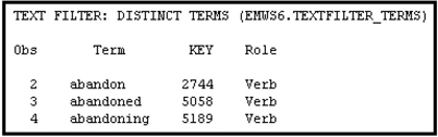
Table 9.12 shows the Transaction data set TextFilter_Transaction, created by the Text Filter node.

Table 9.12

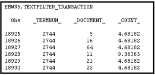
Table 9.13 shows the actual terms associated with the term numbers (keys) and the documents in which the terms occur. Since I set the Frequency Weighting property to None and the Term Weight property to Inverse Document Frequency, the count shown in Table 9.13 is $tfidf$ instead of the raw frequency.

Table 9.13

By transposing the table shown in Table 9.13, you can create a document-term frequency matrix D such as the one shown by Equation 9.1 or a term-document matrix A such as the one shown in Table 9.1 and on the left-hand side of Equation 9.2.

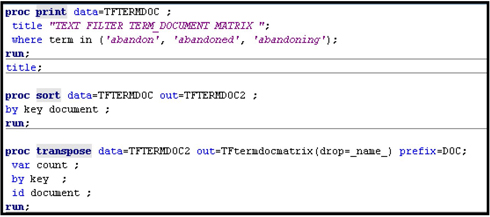
Displays 9.17A – 9.17C show the code used for generating the tables 9.9- 9.13. The code shown in Displays 9.17A – 9.17C is run from the SAS Code node attached to the Text Filter node, as shown in Display 9.15.

Display 9.17A

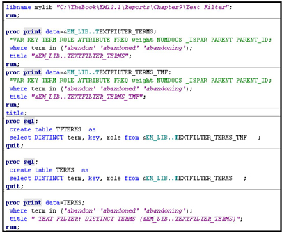
You can view the document data set and the terms used by the Filter node by clicking , located to the right of the Filter Viewer property in the Results group.

Display 9.17B

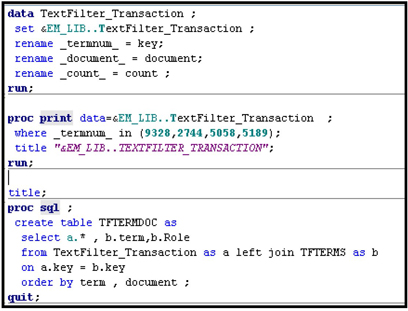
Display 9.17C

9.8 Text Topic Node

The Text Topic node creates topics from the terms collected from the document collection done by the Text Parsing and Text Filter nodes. Different topics are created from different combinations of terms. A Singular Value Decomposition of the term-document matrix is used in creating topics from the terms. Creation of topics from the terms is similar to the derivation of concepts from the term-document matrix using Singular Value Decomposition, demonstrated in Section 9.1.2. Although the procedure used by the Text Topic node may be a lot more complex than the simple illustration I presented in section 9.1.2, the illustration gives a general idea of how the Text Topic node derives topics from the term-document matrix. I recommend that you review Sections 9.1.1 and 9.1.2, with special attention to Equations 9.1 – 9.4, matrices $A,U,\mathrm{\Sigma },V,Dand{D}^{*}$, and Tables 9.1 – 9.4. In the illustrations in Section 9.1.2, I used the term “concept” instead of “topic.” I hope that this switch of terminology does not hamper your understanding of how SVD is used to derive the topics.

Display 9.18 shows the process flow diagram with the Text Topic node connected to the Text Filter node.

Display 9.18

The property settings of the Text Topic node are shown in Display 9.19.

Display 9.19

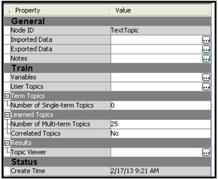
The term-document matrix has 2858 rows (terms) and 77 columns (documents). Selected elements of the -document-term matrix are shown in Table 9.14.

Table 9.14

Tables 9.14A show s the rows corresponding to the term “abandon” (_termnum_ 2744) in the document-term matrix shown in Table 9.14. The term “abandon” is also present in tables 9.5 – 9.11 and 9.13.

Table 9.14A

The Text Topic node derives topics from the term-document matrix (texttopic_tmout_normalized shown in Table 9.14) using Singular Value Decomposition as outlined in Section 9.1.2. In the example presented in this section, 25 topics are derived from the 2858 terms. The topics are shown in Table 9.15.

Table 9.15

The topics shown in Table 9.15 are discovered by the Text Topic node. Alternatively, you can define the topics, include them in a file, and import the file by opening the User Topics window (click , located to the right of User Topics property in the Properties panel).

The Text Topic node creates a data set that you can access from the SAS Code node as &em_lib..TextTopic_train. A partial view of this data set is shown in Table 9.16.

Table 9.16

The last column in Table 9.16 shows the variable TARGET, which takes the value 1 if the author of the paper is Hamilton, and 0 otherwise.

The output data set created by the Text Topic node contains two sets of variables. One set is represented by TextTopic_Rawn and the other by TextTopic_n. For example, for Topic 1, the variables created are TextTopic_Raw1 and TextTopic_1; for Topic 2, Topic 3, etc., they are TextTopic_Raw2 and TextTopic_2, TextTopic_Raw2 and TextTopic_2, etc.

TextTopic_Rawn is the raw score of a document on Topic n, and TextTopic_n is an indicator variable. The variable is set to 1 if TextTopic_Rawn > the document cut-off value (shown in Table 9.15), and is set to 0 if TextTopic_Rawn < the document cut-off value.

You can use TextTopic_Rawn or TextTopic_n in a Logistic Regression, but you should not use both of them at the same time. If you attach a Regression node to the Text Topic node, only the raw scores are passed by the Text Topic node. If you want both the raw scores and the indicator variables to be passed to the next node, you need to attach a Metadata node to the Text Topic node and assign the new role of Input to the indicator variable TextTopic_n (n=1 to 25 in this example).

You can get additional information on the topics by opening the Interactive Topic Viewer window; click located to the right of the Topic Viewer property. The interactive Topic Viewer window opens, as shown in Display 9.20.

Display 9.20

Display 9.20 shows three sections in the Topic Viewer window. Twenty-five topics are listed in the top section. If you scroll down in the top section and click on the 22^nd topic, then the middle section shows the weights of different terms in Topic 22 and the bottom section shows the weight of Topic 22 in different documents.

The term “election” has the highest weight (0.39) in Topic 22. Topic 22 has the highest weight (0.716) in paper 60 which was written by Alexander Hamilton.

9.8.1 Developing a Predictive Equation Using the Output Data Set Created by the Text Topic Node

By connecting a Regression node to the Text Topic node as shown in Display 9.18, you can develop an equation that you can use for predicting who the author of a paper is.

Although I have not done it in this example, in general you should partition the data into Train, Validate, and Test data sets. Since the number of observations is small (77) in the example data set, I used the entire data set for Training only.

In the Regression node, I set the Selection Model property to Stepwise and Selection Criterion to None. With these settings, the model from the final iteration of the Stepwise process is selected. The selected equation is shown in Display 9.21.

Display 9.21

From Display 9.21, you can see that those documents that score high on Topics 10 and 20 are more likely to be authored by Alexander Hamilton.

In order to test the equation shown in Display 9.21, you need a Test data set. As mentioned earlier, I used the entire data set for Training only since there are not enough observations.

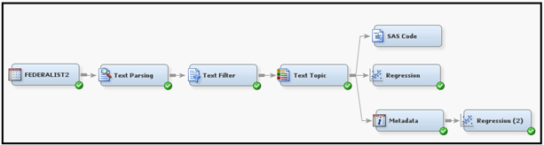
Note that in the logistic regression shown in Display 9.21, only the raw scores are used. I ran an alternative equation using the indicator variables. To make the indicator variables available, I attached the Metadata node to the TextTopic node and attached a Regression node to the Metadata node, as shown in Display 9.22. I set the role of the indicator variables to Input in the Metadata node.

Display 9.22

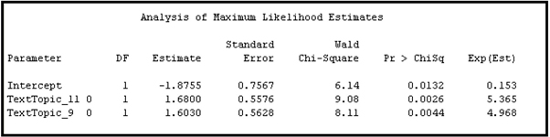
The logistic regression estimated using the indicator variables is shown in Display 9.23.

Display 9.23

9.9 Text Cluster Node

The Text Cluster node divides the documents into non-overlapping clusters. The documents in a cluster are similar with respect to the frequencies of the terms. For developing the clusters, the Text Cluster node makes use of the SVD variables created by using the SVD method, as illustrated in Section 9.1.2. The clusters created are useful in classifying documents. The cluster variable, which indicates which cluster an observation belongs to, can be used as categorical input in predictive modeling.

You can develop clusters using a document-term matrix, also known as the data matrix. The rows of a document-term matrix represent the documents and the columns represent terms, and the cells are raw or weighted frequencies of the terms. If there are $n$ terms and $m$ documents, the term-document matrix is of size $n\times m$ and the data matrix (document-term matrix) is of size $m\times n$. The document-term matrix in our example is of size $77\times 2858$ since there are 77 documents and 2858 terms. The document-term matrix is large and sparse as not all the terms appear in every document. The dimensions of the data matrix are reduced by replacing the terms with SVD variables created by means of Singular Value Decomposition of the term-document matrix, as illustrated in Section 9.1.2. Although in the illustration given in Section 9.1.2 many steps such as normalization and rotation of the vectors are skipped, it is still useful to get a general understanding of how Singular Value Decomposition is used for arriving at the special SVD variables. The number of SVD variables ($p$) is much smaller than the number of terms $n$. As you can see from the data set exported by the Cluster node, the number of SVD terms in this demonstration is 20. That is, $p=20.$ The number of the SVD terms created is determined by the value to which you set the SVD Resolution property. You can set the resolution to Low, Medium, or High. Setting the SVD Resolution property to Low results in the smallest number of SVD variables, and a value of High results in the largest number of SVD variables.

There are two types of clustering available in the Text Cluster node: Hierarchical Clustering andExpectation-Minimization. You can select one of these methods from the Properties panel of the Text Cluster node. Following is a brief explanation of the two methods of clustering.

9.9.1 Hierarchical Clustering

If you set the Cluster Algorithm property to Hierarchical Clustering, the Text Cluster nodes uses Ward’s method⁶ for creating the clusters. In this method, the observations (documents) are progressively combined into clusters in such a way that an objective function is minimized at each combination step. The error sum of squares for the $k^{th}$ cluster is:

 

$$E_k={\displaystyle \sum _{i=1}^{m_k}{\displaystyle \sum _{j=1}^p{\left(x_{ijk}-{\overline{x}}_{jk}\right)}^2}}(9.5)$$

Where:

$E_k=$ Error sum of squares for the $k^{th}$ cluster

$x_{ijk}=$ Value of the $j^{th}$ variable at the $i^{th}$ observation in the $k^{th}$ cluster

${\overline{x}}_{jk}=$ Mean of the $j^{th}$ variable in the $k^{th}$ cluster

$m_k=$ Number of observations (documents) in the $k^{th}$ cluster

$p=$ Number of variables used for clustering

The objective function is the combined Error Sums of Squares given by:

 

$$E={\displaystyle \sum _{k=1}^K{E}_k}(9.6)$$

Where:

$K=$ Number of clusters

At each step, the union of every possible pair of clusters is considered, and the two clusters whose union results in the minimum increase in the error sum of squares ($E$) are combined.

If the clusters $u$ and $v$ are combined to form a single cluster $w$, then the increase in error resulting from the union of clusters $u$ and $v$ is given by:

$$\Delta E_{uv}=E_w-\left(E_u+E_v\right)(9.7)$$

Where:

$\Delta E_{uv}=$ Increase in the Error sum of squares due to combining clusters $u$ and $v$

$E_w=$ Error sum of squares for cluster $w$, which is the union of clusters $u$ and $v$

$E_u=$ Error sum of squares for cluster $u$

$E_v=$ Error sum of squares for cluster $v$

Initially, each observation (document) is regarded as a cluster, and the observations are progressively combined into clusters as described above.

9.9.2 Expectation-Maximization (EM) Clustering

The Expectation-Maximization algorithm assumes a probability density function of the variables in each cluster. If $X$ is a vector of $p$ random variables, then the joint probability distribution of the random vector $X$ in cluster $k$ can be written as $f_k(X|{\theta }_k)$, where ${\theta }_k$ is a set of parameters that characterize the probability distribution. If we assume that the random vector $X$ has a joint normal distribution, the parameters ${\theta }_k$ consist of a mean vector ${\mu }_k$ and a variance-covariance matrix ${\mathrm{\Sigma }}_k$, and the joint probability density function of $X$ in cluster $k$ is given by:

 

$$f_k\left(X|{\mu }_k,{\mathrm{\Sigma }}_k\right)=\frac{1}{\sqrt{{\left(2\pi \right)}^p\left|{\mathrm{\Sigma }}_k\right|}}\exp \left[-\frac{1}{2}{\left(X-{\mu }_k\right)}^{\prime }{\left(\mathrm{\Sigma }\right)}^{-1}\left(X-{\mu }_k\right)\right](9.8)$$

The probability density function for cluster $k$ given in Equation 9.8 can be evaluated at any observation point by replacing the random vector $X$ with the observed data vector $x$, as shown in Equation 9.9:

 

$$f_k\left(x|{\mu }_k,{\mathrm{\Sigma }}_k\right)=\frac{1}{\sqrt{{\left(2\pi \right)}^p\left|{\mathrm{\Sigma }}_k\right|}}\exp \left[-\frac{1}{2}{\left(x-{\mu }_k\right)}^{\prime }{\left(\mathrm{\Sigma }\right)}^{-1}\left(x-{\mu }_k\right)\right](9.9)$$

We need estimates of the parameters ${\mu }_k\text{ and }{\mathrm{\Sigma }}_k$ in order to calculate the probability density function given by Equation 9.8. These parameters are estimated iteratively in EM algorithm. The probability density functions given in Equations 9.8 and 9.9 are conditional probability density functions. The unconditional probability density function evaluated at an observation is:

$$p(x)={\displaystyle \sum _{k=1}^K{\pi }_k{f}_k(x|{\mu }_k,{\mathrm{\Sigma }}_k)}(9.10)$$

where ${\pi }_k$ is the probability of cluster $k$, as defined in the following illustration.

9.9.2.1 An Example of Expectation-Maximization Clustering

In order to demonstrate Expectation-Maximization Clustering, I generated an example data set consisting of 200 observations (documents). I generated the example data set from a mixture of two univariate normal distributions so that the data set contains only one input (x), which can be thought of as a measure of document strength in a given concept. My objective is to create two clusters of documents based on the single input. Initially I assigned the documents randomly to two clusters: Cluster A and Cluster B. Starting from these random, initial clusters, the Expectation-Maximization algorithm iteratively produced two distinct clusters. The iterative steps are given below:

Iteration 0 (Initial random clusters)

1. Assign observations randomly to two clusters A and B. These arbitrary clusters are needed to start the EM iteration process.

2. Define two weight variables $w_{ai}(0)$ and $w_{bi}(0)$ as follows:
$w_{ai}(0)=$ 1, if the $i^{th}$ observation is assigned to cluster A
$w_{ai}(0)=$ 0, otherwise.
$w_{bi}(0)=$ 1, if the $i^{th}$ observation is assigned to cluster B
$w_{bi}(0)=$ 0 otherwise
(The 0 in the brackets indicates the iteration number.)

3. Calculate the cluster probabilities ${\pi }_a(0)$ and ${\pi }_b(0)$ as

 

$$\begin{array}{l}{\pi }_a(0)=\frac{{\displaystyle \sum _{i=1}^n{w}_{ai}(0)}}{n}\text{ and}\\ {\pi }_b(0)=\frac{{\displaystyle \sum _{i=1}^n{w}_{bi}(0)}}{n},\end{array}$$

where $n$ is number of observations (200 in this example).

4. Calculate cluster means ${\mu }_j(0)$ and cluster standard deviations ${\sigma }_j(0)$, where the subscript $j$ stands for a cluster and 0 in the brackets indicates the iteration number. Since we are considering only two clusters in this example, $j$ takes the values $a$ and $b$.

 

$${\mu }_a(0)=\frac{{\displaystyle \sum _{i=1}^n(w_{ai}(0))x_i}}{{\displaystyle \sum _{i=1}^n{w}_{ai}(0)}}\text{,}$$

where $x_i$ is the value of the input variable for observation (document) $i$, $w_{ai}$ is the value of the weight variable (as defined in Step 2) for observation $i$, and ${\mu }_a(0)$ is the mean of the input variable for cluster A at iteration 0.

Similarly, the mean of the input variable for Cluster B is calculated as:

 

$${\mu }_b(0)=\frac{{\displaystyle \sum _{i=1}^n(w_{bi}(0))x_i}}{{\displaystyle \sum _{i=1}^n{w}_{bi}(0)}}$$

The standard deviations ${\sigma }_a(0)$ and ${\sigma }_b(0)$ for clusters A and B are calculated as

${\sigma }_a{}^2(0)=\frac{{\displaystyle \sum _{i=1}^n(w_{ai}(0)){(x_i-{\mu }_a(0))}^2}}{{\displaystyle \sum _{i=1}^n{w}_{ai}(0)}}$ and ${\sigma }_b{}^2(0)=\frac{{\displaystyle \sum _{i=1}^n(w_{bi}(0)){(x_i-{\mu }_{ba}(0))}^2}}{{\displaystyle \sum _{i=1}^n{w}_{bi}(0)}}$ respectively.

Iteration 1

1. Calculate the probabilities of cluster membership of the $i^{th}$ observation:

 

$$\begin{array}{l}P\left(A|x_i\right)=P\left(x_i|A\right)P(A)=f_A(x_i){\pi }_a(0)\text{ and}\\ P\left(B|x_i\right)=P\left(x_i|B\right)P(B)=f_B(x_i){\pi }_b(0)\\ \end{array}$$

where

$\begin{array}{l}{f}_A(x_i)=pdf\left(\text{'}Normal\text{'},x_i,{\mu }_a(0),{\sigma }_a(0)\right)\text{ and}\\ f_B(x_i)=pdf\left(\text{'}Normal\text{'},x_i,{\mu }_b(0),{\sigma }_b(0)\right).\end{array}$

2. Calculate the weights for the $i^{th}$ observation:

$$\begin{array}{l}{w}_{ai}(1)=\frac{P(A|x_i)}{P(A|x_i)+P(B|x_i)}\text{ and}\\ w_{bi}(1)=\frac{P(B|x_i)}{P(A|x_i)+P(B|x_i)}.\end{array}$$

(Since $w_{ai}(1)+w_{bi}(1)=1$ at each observation, ${\displaystyle \sum _{i=1}^n{w}_{ai}(1)+}{\displaystyle \sum _{i=1}^n{w}_{bi}(1)=n}$= total number of observations in the data set. This is true at each iteration).

3. Calculate the log-likelihood of the $i^{th}$ observation:

 

$$L_i=\log \left(P(A|x_i)+P(B|x_i)\right)$$

4. Calculate the log-likelihood for this iteration:

 

$$L{L}_i={\displaystyle \sum _{i=1}^n{L}_i}$$

5. Calculate cluster probabilities:

 

$${\pi }_a(1)=\frac{{\displaystyle \sum _{i=1}^n{w}_{ai}(1)}}{n}\text{ ,}{\pi }_b(1)=\frac{{\displaystyle \sum _{i=1}^n{w}_{bi}(1)}}{n}$$

6. Calculate cluster means:

 

$${\mu }_a(1)=\frac{{\displaystyle \sum _{i=1}^n(w_{ai}(1))x_i}}{{\displaystyle \sum _{i=1}^n{w}_{ai}(1)}}\text{ and }{\mu }_b(1)=\frac{{\displaystyle \sum _{i=1}^n(w_{bi}(1))x_i}}{{\displaystyle \sum _{i=1}^n{w}_{bi}(1)}}$$

7. Calculate cluster standard deviations:

${\sigma }_a{}^2(1)=\frac{{\displaystyle \sum _{i=1}^n(w_{ai}(1)){(x_i-{\mu }_a(1))}^2}}{{\displaystyle \sum _{i=1}^n{w}_{ai}(1)}}$ and ${\sigma }_b{}^2(1)=\frac{{\displaystyle \sum _{i=1}^n(w_{bi}(1)){(x_i-{\mu }_b(1))}^2}}{{\displaystyle \sum _{i=1}^n{w}_{bi}(1)}}$.

Iteration 2

1. Calculate the probabilities of cluster membership of the $i^{th}$ observation:

 

$$\begin{array}{l}P\left(A|x_i\right)=P\left(x_i|A\right)P(A)=f_A(x_i){\pi }_a(1)\text{ and}\\ P\left(B|x_i\right)=P\left(x_i|B\right)P(B)=f_b(x_i){\pi }_b(1)\end{array}$$

where

 

$$\begin{array}{l}{f}_A(x_i)=pdf\left(\text{'}Normal\text{'},x_i,{\mu }_a(1),{\sigma }_a(1)\right)\text{ and}\\ f_B(x_i)=pdf\left(\text{'}Normal\text{'},x_i,{\mu }_b(1),{\sigma }_b(1)\right).\end{array}$$

2. Calculate the weights:

 

$$\begin{array}{l}{w}_{ai}(2)=\frac{P(A|x_i)}{P(A|x_i)+P(B|x_i)}\text{ and}\\ w_{bi}(2)=\frac{P(B|x_i)}{P(A|x_i)+P(B|x_i)}.\end{array}$$

3. Calculate the log-likelihood of the $i^{th}$ observation:

 

$$L_i=\log \left(P(A|x_i)+P(B|x_i)\right)$$

4. Calculate the log-likelihood for this iteration:

 

$$L{L}_i={\displaystyle \sum _{i=1}^n{L}_i}$$

5. Calculate cluster probabilities:

 

$${\pi }_a(2)=\frac{{\displaystyle \sum _{i=1}^n{w}_{ai}(2)}}{n}\text{ ,}{\pi }_b(2)=\frac{{\displaystyle \sum _{i=1}^n{w}_{bi}(2)}}{n}$$

Since $w_{ai}(2)+w_{bi}(2)=1$ at each observation, $n={\displaystyle \sum _{i=1}^n{w}_{ai}(2)+}{\displaystyle \sum _{i=1}^n{w}_{bi}(2)}$ at each iteration.

6. Calculate cluster means:

 

$${\mu }_a(2)=\frac{{\displaystyle \sum _{i=1}^n(w_{ai}(2))x_i}}{{\displaystyle \sum _{i=1}^n{w}_{ai}(2)}}\text{ and }{\mu }_b(2)=\frac{{\displaystyle \sum _{i=1}^n(w_{bi}(2))x_i}}{{\displaystyle \sum _{i=1}^n{w}_{bi}(2)}}$$

7. Calculate cluster standard deviations:

${\sigma }_a{}^2(2)=\frac{{\displaystyle \sum _{i=1}^n(w_{ai}(2)){(x_i-{\mu }_a(2))}^2}}{{\displaystyle \sum _{i=1}^n{w}_{ai}(2)}}$ and ${\sigma }_b{}^2(2)=\frac{{\displaystyle \sum _{i=1}^n(w_{bi}(2)){(x_i-{\mu }_b(2))}^2}}{{\displaystyle \sum _{i=1}^n{w}_{bi}(2)}}$.

You can calculate cluster probabilities, the weights, cluster probabilities and the parameters of the probability distributions in iteration 3, iteration 4 …etc.

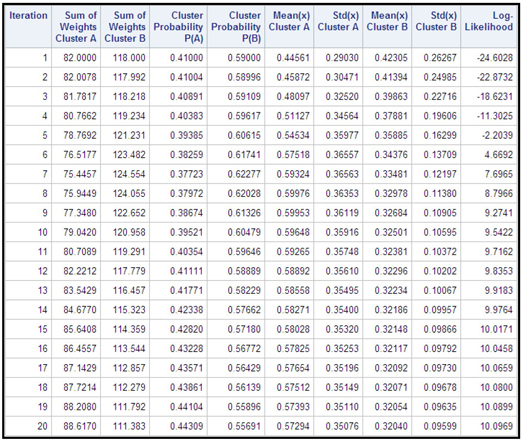
In the example shown below, the data set has 200 observations and a single input (x) drawn from a mixture of two univariate normal distributions. The EM algorithm is applied iteratively, as described above, to create two clusters. Table 9.18 shows the results of 20 iterations.

Table 9.17

Display 9.24 shows a plot of log-likelihood by iteration.

Display 9.24

As Table 9.17 and Display 9.24 show, the likelihood increases rapidly from -24.6 in iteration 1 to 7.6965 in iteration 7. After iteration 7, the rate of change in log-likelihood diminishes steadily and log-likelihood becomes increasingly flatter. The difference in the likelihood between iterations 19 and 20 is only 0.007, showing that the solution converged by iteration 19.

Using the weights calculated in the final iteration, I assigned $i^{th}$ observation to Cluster 1 if $w_{ai}(20)\text{ > }{w}_{bi}(20)$ and to cluster 2 if $w_{ai}(20)\le w_{bi}(20)$. The means and the standard deviations of the variable X in the clusters are shown in Table 9.18.

Table 9.18

Table 9.18 shows that the mean of the variable x is higher for Cluster 1 than for Cluster 2. Starting with an arbitrary set of clusters, we arrived at two distinct clusters.

In our example, there is only one input, namely, $x$ which is continuous. In calculating the likelihood of each observation, we used normal probability density functions. If you have several continuous variables, you can use a separate normal density function for each variable if they are independent, or you can use a joint normal density function if they are jointly distributed. For ordinal variables, you can use geometric or Poisson distributions and for other categorical variables you can use multinomial distribution. The Expectation-Maximization clustering can be used with variables of different measurement scales by choosing the appropriate probability distributions.

The method outlined can be extended to more than one variable.

For another illustration of the EM algorithm, refer to Data Mining the Web,⁷ by Markov and Larose.

9.9.3 Using the Text Cluster Node

Display 9.25 shows the process diagram with two instances of the Text Cluster node. In the first instance, I generated clusters using the Hierarchical Clustering algorithm, and in the second instance I generated clusters using the Expectation-Maximization Clustering algorithm.

Display 9.25

9.9.3.1 Hierarchical Clustering

Display 9.26 shows the properties of the first instance of the Text Cluster node.

Display 9.26

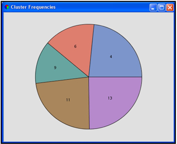
With the property settings shown in Display 9.26, the Text Cluster node produced five clusters. The cluster frequencies are shown in Display 9.27.

Display 9.27

Display 9.28 shows a list of the descriptive terms of each cluster.

Display 9.28

The target variable in the data set is Target, which takes the value 1 if the author of the paper is Alexander Hamilton and 0 otherwise. Table 9.19 shows the cross tabulation of the clusters and the target variable.

Table 9.19

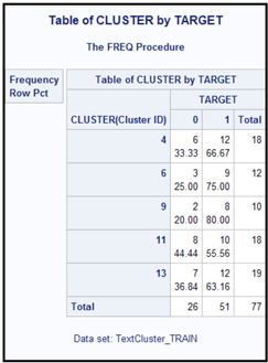
You can see n that Clusters 6 and 9 are dominated by the papers written by Alexander Hamilton.

9.9.3.2 Expectation-Maximization Clustering

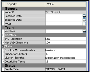
Display 9.29 shows the properties settings of the second instance of the Text Cluster node.

Display 9.29

Display 9.30 shows the cluster frequencies.

Display 9.30

Display 9.31 shows the descriptive terms of the clusters.

Display 9.31

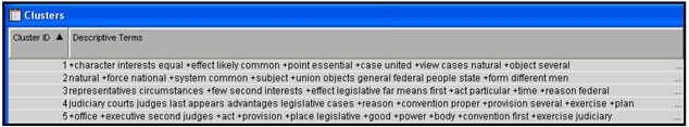
Table 9.20 shows the cross tabulation of the clusters and the target variable.

Table 9.20

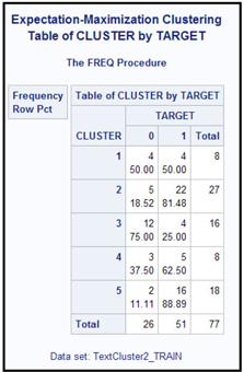
Clusters 2 and 5 are dominated by papers written by Hamilton.

9.10 Exercises

1. Collect URLs by typing the words “Economy,” “GDP,” “Unemployment Rate,” and “European Debt” in Google search. Search for each word separately and collect 5 or 10 links for each word.

2. Repeat the same for the words “health,” “vitamins,” “Medical,” and “health insurance.”

3. Use %TMFILTER to download web pages, as shown in Display 9.1. Store the pages as text files in different directories

4. Use %TMFILTER to create SAS data sets, as shown Display 9.5. Include a target variable Target, which takes the value 1 for the documents relating to Economics and 0 for the documents not related to Economics.

5. Create a data source.

6. Create a process flow diagram as shown in Display 9.22.

7. Run the nodes in succession, and finally run the Regression node.
Do the logistic regression results make sense? If not, why not?

Notes

1. The text mining nodes are only available if you license SAS Text Miner.

2. A full Singular Value Decomposition of an $m\times n$ matrix results in a $U$ matrix of size $m\times n$, a $\mathrm{\Sigma }$ matrix of size $n\times m$ and a $V$ matrix of size $n\times m$. Since I have used a reduced Singular Value Decomposition, the dimensions of the matrices are smaller.

3. Character strings without blank spaces are called tokens.

4. The root or stem of the words “is” and “are” is “be”.

5. The document-term matrix is a data set that is in a spreadsheet format where the rows represent the documents, columns represent the terms, and the cells show the adjusted frequency of occurrence of the terms in each document.

6. A clear exposition of the Ward’s method can be found in Wishart, David. “An Algorithm for Hierarchical Classifications.” Biometrics Vol. 25, No.1 (March 1969: 165-170.

7. Markov, Zdravko and Daniel T. Larose. 2007. Data Mining the Web Uncovering Patterns in Web Content, Structure, and Usage. Wiley-Interscience.