This chapter explores the Regression node in detail using two practical business applications—one requiring a model to predict a binary target and the other requiring a model to predict a continuous target. Before developing these two models, I present an overview of the types of models that can be developed in the Regression node, the theory and rationale behind each type of model, and an explanation of how to set various properties of the Regression node to get the desired models.

6.2 What Types of Models Can Be Developed Using the Regression Node?

6.2.1 Models with a Binary Target

When the target is binary, either numeric or character, the Regression node estimates a logistic regression. The Regression node produces SAS code to calculate the probability of the event (such as response or attrition). The computation of the probability of the event is done through a link function. A link function shows the relation between the probability of the event and a linear predictor, which is a linear combination of the inputs (explanatory variables).

The linear predictor can be written as $β^{'} x$ $β^{'} x$ , where $x$ $x$ is a vector of inputs and $β$ $β$ is the vector of coefficients estimated by the Regression node. For a response model, where the target takes on a value of 1 or 0 (1 stands for response and 0 for non-response), the link function is

\log (\frac{\Pr (y = 1 | x)}{1 - \Pr (y = 1 | x)}) = β^{'} x (6.1)

$\log (\frac{\Pr (y = 1 | x)}{1 - \Pr (y = 1 | x)}) = β^{'} x (6.1)$

where $y$ $y$ is the target and $\Pr (y = 1 | x)$ $\Pr (y = 1 | x)$ is the probability of the target variable taking the value 1 for a customer (or a record in the data set), given the values of the inputs or explanatory variables for that customer. The left-hand side of Equation 6.1 is the logarithm of odds or log-odds of the event “response”. Since Equation 6.1 shows the relation between the log-odds of the event and the linear predictor $β^{'} x$ $β^{'} x$ , it is called a logit link.

If you solve the link function given in Equation 6.1 for $\Pr (y = 1 | x)$ $\Pr (y = 1 | x)$ , you get:

\Pr (y = 1 | x) = \frac{\exp (β^{'} x)}{1 + \exp (β^{'} x)} (6.2)

$\Pr (y = 1 | x) = \frac{\exp (β^{'} x)}{1 + \exp (β^{'} x)} (6.2)$

Equation 6.2 is called the inverse link function. In Chapter 5, where we discussed neural networks, we called equations of this type activation functions.

From Equation 6.2, you can see that

1 - \Pr (y = 1 | x) = 1 - \frac{\exp (β^{'} x)}{1 + \exp (β^{'} x)} = \frac{1}{1 + \exp (β^{'} x)} (6.3)

$1 - \Pr (y = 1 | x) = 1 - \frac{\exp (β^{'} x)}{1 + \exp (β^{'} x)} = \frac{1}{1 + \exp (β^{'} x)} (6.3)$

Dividing Equation 6.3 by Equation 6.2 and taking logs, I once again obtain the logit link given in Equation 6.1.

The important feature of this function for our purposes is that it produces values that lie only between 0 and 1, just as the as the probability of response and non-response do.

In addition to the logit link, the Regression node provides probit and complementary log-log link functions. (These are discussed in Section 6.3.2.) All of these link functions keep the predicted probabilities between 0 and 1. In cases where it is not appropriate to constrain the predicted values to lie between 0 and 1, no link function is needed.

There are also some well-accepted theoretical rationales behind some of these link functions. For readers who are interested in pursuing this line of reasoning further, a discussion of the theory is included in Section 6.3.2.

Display 6.1 shows the process flow diagram for a regression with a binary target.

Display 6.1

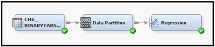
Display 6.2 shows a partial list of the variables in the input data set used in this process flow. You can see from Display 6.2 that the target variable RESP is binary.

Display 6.2

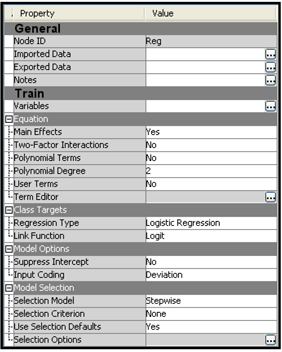
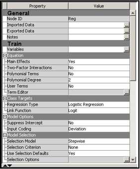
Display 6.3 shows the properties of the Regression node that is in the process flow.

Display 6.3

After running the Regression node, you can open the SAS code from the Results window by clicking View→Scoring→SAS code.

Displays 6.4A and 6.4B show the SAS code used for calculating the linear predictor and the probabilities of response and no response for each record in a Score data set.

Display 6.4A

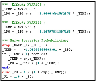
Display 6.4B

In Display 6.4A, _LPO is the linear combination of the inputs and _TEMP =_LPO + the estimated intercept (-4.54086566603301). _TEMP is the linear predictor $β^{'} x$ $β^{'} x$ shown in Equation 6.1.

You learn more about modeling binary targets in Section 6.4, where a model with a binary target is developed for a marketing application.

6.2.2 Models with an Ordinal Target

Ordinal targets, also referred to as ordered polychotomous targets, take on more than two discrete, ordered values. An example of an ordinal target with three levels (0, 1, and 2) is the discretized version of the loss frequency variable discussed in Chapter 5.

If you want your target to be treated as an ordinal variable, you must set its measurement scale to Ordinal. However, if the target variable has fewer than the number of levels specified in the Advanced Advisor Metadata options, SAS Enterprise Miner sets its measurement scale to Nominal (see Section 2.5, Displays 2.10 and 2.11). If the measurement scale of your target variable is currently set to Nominal but you want to model it as an ordinal target, then you must change its measurement scale setting to Ordinal. In the Appendix to Chapter 3, I showed how to change the measurement scale of a variable in a data source.

When the target is ordinal, then, by default, the Regression node produces a Proportional Odds (or Cumulative Logits) model, as discussed in Chapter 5, Section 5.5.1.1. (The following example illustrates the proportional odds model as well.) When the target is nominal, on the other hand, it produces a Generalized Logits model, which is presented in Section 6.2.3. Although the default value of the Regression Type property is Logistic Regression and the default value of the Link Function property (link functions are discussed in detail in Section 6.3.2) is Logit for both ordinal targets and nominal targets, the models produced are different for targets with different measurement scales. Hence, the setting of the measurement scale determines which type of model you get. Using some simple examples, I will demonstrate how different types of models are produced for different measurement scales even though the Regression node properties are all set to the same values.

Display 6.5 shows the process flow for a regression with an ordinal target.

Display 6.5

Display 6.6 shows the list of variables and their measurement scales, or levels. In the second and third columns, you can see that the role of the variable $L O S S F R Q$ $L O S S F R Q$ is a target and its measurement scale (level) is ordinal.

Display 6.6

Display 6.7 shows the Properties panel of the Regression node in the process flow shown in Display 6.5.

Display 6.7

Note the settings in the Class Targets section. These settings are the default values for class targets (categorical targets), including binary, ordinal, and nominal targets. Since the target variable $L O S S F R Q$ $L O S S F R Q$ is ordinal, taking on the values 0, 1, or 2 for any given record of the data set, the Regression node uses a cumulative logits link.

The expression $\frac{\Pr (l o s s f r q = 2)}{1 - \Pr (l o s s f r q = 2)}$ $\frac{\Pr (l o s s f r q = 2)}{1 - \Pr (l o s s f r q = 2)}$ is called the odds ratio. It is the odds that the event $L O S S F R Q$ $L O S S F R Q$ =2 will occur. In other words, the odds ratio represents the odds of the loss frequency equaling 2. Similarly, the expression $\frac{\Pr (l o s s f r q = 1) + \Pr (l o s s f r q = 2)}{1 - {\Pr (l o s s f r q = 1) + \Pr (l o s s f r q = 2)}}$ $\frac{\Pr (l o s s f r q = 1) + \Pr (l o s s f r q = 2)}{1 - {\Pr (l o s s f r q = 1) + \Pr (l o s s f r q = 2)}}$ represents the odds of the event $L O S S F R Q$ $L O S S F R Q$ =1 or 2. When I take the logarithms of the above expressions, they are called log-odds or logits.

Thus the logit for the event $L O S S F R Q$ $L O S S F R Q$ =2 is $\log (\frac{\Pr (l o s s f r q = 2)}{1 - \Pr (l o s s f r q = 2)})$ $\log (\frac{\Pr (l o s s f r q = 2)}{1 - \Pr (l o s s f r q = 2)})$ , and the logit for the event $L O S S F R Q$ $L O S S F R Q$ =1 or 2 is $\log (\frac{\Pr (l o s s f r q = 1) + \Pr (l o s s f r q = 2)}{1 - {\Pr (l o s s f r q = 1) + \Pr (l o s s f r q = 2)}})$ $\log (\frac{\Pr (l o s s f r q = 1) + \Pr (l o s s f r q = 2)}{1 - {\Pr (l o s s f r q = 1) + \Pr (l o s s f r q = 2)}})$ .

The logits shown above are called cumulative logits. When a cumulative logits link is used, the logits of the event $L O S S F R Q$ $L O S S F R Q$ =1 or 2 are larger than the logits for the event $L O S S F R Q$ $L O S S F R Q$ =2 by a positive amount. In a Cumulative Logits model, the logits of the event $L O S S F R Q$ $L O S S F R Q$ =2 and the event $L O S S F R Q$ $L O S S F R Q$ =1 or 2 differ by a constant amount for all observations (all customers). To illustrate this phenomenon, I run the Regression node with an ordinal target ( $L O S S F R Q$ $L O S S F R Q$ ). Display 6.8, which is taken from the Results window, shows the equations estimated by the Regression node.

Display 6.8

From the coefficients given in Display 6.8, I can write the following two equations:¹

\begin{array}{l} \log (\frac{\Pr (l o s s f r q = 2)}{1 - \Pr (l o s s f r q = 2)}) = - 2.8840 - 0.0231 * A G E - 0.00498 * C R E D (6.4) \\ + 0.2252 * N P R V I O \end{array}

$\begin{array}{l} \log (\frac{\Pr (l o s s f r q = 2)}{1 - \Pr (l o s s f r q = 2)}) = - 2.8840 - 0.0231 * A G E - 0.00498 * C R E D (6.4) \\ + 0.2252 * N P R V I O \end{array}$

\begin{array}{l} \log (\frac{\Pr (l o s s f r q = 2) + \Pr (l o s s f r q = 1)}{1 - {\Pr (l o s s f r q = 2) + \Pr (l o s s f r q = 1)}}) = 0.2133 - 0.0231 * A G E - 0.00498 * C R E D (6.5) \\ + 0.2252 * N P R V I O \end{array}

$\begin{array}{l} \log (\frac{\Pr (l o s s f r q = 2) + \Pr (l o s s f r q = 1)}{1 - {\Pr (l o s s f r q = 2) + \Pr (l o s s f r q = 1)}}) = 0.2133 - 0.0231 * A G E - 0.00498 * C R E D (6.5) \\ + 0.2252 * N P R V I O \end{array}$

To interpret the results, take the example of a customer (Customer A) who is 50 years of age (AGE=50), has a credit score of 670(CRED=670), and has two prior traffic violations (NPRVIO=2).

From Equation 6.4, the log-odds (logit) of the event $L O S S F R Q$ $L O S S F R Q$ =2 for Customer A are:

\log (\frac{\Pr (l o s s f r q = 2}{1 - \Pr (l o s s f r q = 2}) = - 2.8840 - 0.0231 * 50 - 0.00498 * 670 + 0.2252 * 2 (6.4A)

$\log (\frac{\Pr (l o s s f r q = 2}{1 - \Pr (l o s s f r q = 2}) = - 2.8840 - 0.0231 * 50 - 0.00498 * 670 + 0.2252 * 2 (6.4A)$

Therefore, the odds of the event $L O S S F R Q$ $L O S S F R Q$ =2 for Customer A are

(\frac{\Pr (l o s s f r q = 2)}{1 - \Pr (l o s s f r q = 2)}) = e^{- 2.8840 - 0.0231 * 50 - 0.00498 * 670 + 0.2252 * 2} (6.4 B)

$(\frac{\Pr (l o s s f r q = 2)}{1 - \Pr (l o s s f r q = 2)}) = e^{- 2.8840 - 0.0231 * 50 - 0.00498 * 670 + 0.2252 * 2} (6.4 B)$

From Equation 6.5, the log-odds (logit) of the event $L O S S F R Q$ $L O S S F R Q$ =1 or 2 for Customer A are:

\begin{array}{l} \log (\frac{\Pr (l o s s f r q = 2) + \Pr (l o s s f r q = 1)}{1 - {\Pr (l o s s f r q = 2) + \Pr (l o s s f r q = 1)}}) = 0.2133 - 0.0231 * 50 - 0.00498 * 670 (6.5 A) \\ + 0.2252 * 2 \end{array}

$\begin{array}{l} \log (\frac{\Pr (l o s s f r q = 2) + \Pr (l o s s f r q = 1)}{1 - {\Pr (l o s s f r q = 2) + \Pr (l o s s f r q = 1)}}) = 0.2133 - 0.0231 * 50 - 0.00498 * 670 (6.5 A) \\ + 0.2252 * 2 \end{array}$

The odds of the event $L O S S F R Q$ $L O S S F R Q$ =1 or 2 for Customer A is

(\frac{\Pr (l o s s f r q = 2) + \Pr (l o s s f r q = 1)}{1 - {\Pr (l o s s f r q = 2) + \Pr (l o s s f r q = 1)}}) = e^{0.2133 - 0.0231 * 50 - 0.00498 * 670 + 0.2252 * 2} (6.5 B)

$(\frac{\Pr (l o s s f r q = 2) + \Pr (l o s s f r q = 1)}{1 - {\Pr (l o s s f r q = 2) + \Pr (l o s s f r q = 1)}}) = e^{0.2133 - 0.0231 * 50 - 0.00498 * 670 + 0.2252 * 2} (6.5 B)$

The difference in the logits (not the odds, but the log-odds) for the events $L O S S F R Q$ $L O S S F R Q$ =1 or 2 and $L O S S F R Q$ $L O S S F R Q$ = 2 is equal to 0.2133–(–2.8840) =3.0973, which is obtained by subtracting Equation 6.4A from Equation 6.5A. Irrespective of the values of the inputs AGE, CRED, and NPRVIO, the difference in the logits (or logit difference) for the events $L O S S F R Q$ $L O S S F R Q$ =1 or 2 and = 2 is the same constant 3.0973. Now turning to the odds of the event, rather than the log-odds, if I divide Equation 6.5B by 6.4B, I get the ratio of the odds of the event $L O S S F R Q$ $L O S S F R Q$ =1 or 2 to the odds of the event $L O S S F R Q$ $L O S S F R Q$ =2. This ratio is equal to

\frac{e^{0.2133}}{e^{- 2.8840}} = e^{0.2133 + 2.8840} = e^{3.0973} = 22.1381.

$\frac{e^{0.2133}}{e^{- 2.8840}} = e^{0.2133 + 2.8840} = e^{3.0973} = 22.1381.$

By this result, I can see that the odds of the event $L O S S F R Q$ $L O S S F R Q$ =1 or 2 is proportional to the odds of the event $L O S S F R Q$ $L O S S F R Q$ = 2, and that the proportionality factor is 22.1381. This proportionality factor is the same for any values of the inputs (AGE, CRED, and NPRVIO in this example). Hence the name is Proportional Odds model.

Now I compare these results to those for Customer B, who is the same age (50) and has the same credit score (670) as Customer A, but who has three prior violations (NPRVIO=3) instead of two. In other words, all of the inputs except for NPRVIO are the same for Customer B and Customer A. I show how the log-odds and the odds for the events $L O S S F R Q$ $L O S S F R Q$ =2 and $L O S S F R Q$ $L O S S F R Q$ = 1 or 2 for Customer B differ from those for Customer A.

From Equation 6.4, the log-odds (logit) of the event $L O S S F R Q$ $L O S S F R Q$ =2 for Customer B are:

\begin{array}{l} \log (\frac{\Pr (l o s s f r q = 2)}{1 - \Pr (l o s s f r q = 2)}) = - 2.8840 - 0.0231 * 50 - 0.00498 * 670 (6.4 C) \\ + 0.2252 * 3 \end{array}

$\begin{array}{l} \log (\frac{\Pr (l o s s f r q = 2)}{1 - \Pr (l o s s f r q = 2)}) = - 2.8840 - 0.0231 * 50 - 0.00498 * 670 (6.4 C) \\ + 0.2252 * 3 \end{array}$

Therefore, the odds of the event $L O S S F R Q$ $L O S S F R Q$ =2 for Customer B are:

(\frac{\Pr (l o s s f r q = 2)}{1 - \Pr (l o s s f r q = 2)}) = e^{- 2.8840 - 0.0231 * 50 - 0.00498 * 670 + 0.2252 * 3} (6.4 D)

$(\frac{\Pr (l o s s f r q = 2)}{1 - \Pr (l o s s f r q = 2)}) = e^{- 2.8840 - 0.0231 * 50 - 0.00498 * 670 + 0.2252 * 3} (6.4 D)$

From Equation 6.5, the log-odds (logit) of the event $L O S S F R Q$ $L O S S F R Q$ =1 or 2 for Customer B are:

\begin{array}{l} \log (\frac{\Pr (l o s s f r q = 2) + \Pr (l o s s f r q = 1)}{1 - {\Pr (l o s s f r q = 2) + \Pr (l o s s f r q = 1)}}) = 0.2133 - 0.0231 * 50 - 0.00498 * 670 (6.5 C) \\ + 0.2252 * 3 \end{array}

$\begin{array}{l} \log (\frac{\Pr (l o s s f r q = 2) + \Pr (l o s s f r q = 1)}{1 - {\Pr (l o s s f r q = 2) + \Pr (l o s s f r q = 1)}}) = 0.2133 - 0.0231 * 50 - 0.00498 * 670 (6.5 C) \\ + 0.2252 * 3 \end{array}$

The odds of the event $L O S S F R Q$ $L O S S F R Q$ =1 or 2 for Customer B are:

(\frac{\Pr (l o s s f r q = 2) + \Pr (l o s s f r q = 1)}{1 - {\Pr (l o s s f r q = 2) + \Pr (l o s s f r q = 1)}}) = e^{0.2133 - 0.0231 * 50 - 0.00498 * 670 + 0.2252 * 3} (6.5 D)

$(\frac{\Pr (l o s s f r q = 2) + \Pr (l o s s f r q = 1)}{1 - {\Pr (l o s s f r q = 2) + \Pr (l o s s f r q = 1)}}) = e^{0.2133 - 0.0231 * 50 - 0.00498 * 670 + 0.2252 * 3} (6.5 D)$

It is clear that the difference between log-odds of the event $L O S S F R Q$ $L O S S F R Q$ =2 for Customer B and Customer A is 0.2252, which is obtained by subtracting 6.4A from 6.4C.

It is also clear that the difference between log-odds of the event $L O S S F R Q$ $L O S S F R Q$ =1 or 2 for Customer B and Customer A is also 0.2252, which is obtained by subtracting 6.5A from 6.5C.

The difference in the log-odds (0.2252) is simply the coefficient of the variable NPRVIO, whose value differs by 1 for customers A and B. Generalizing this result, we now see that the coefficient of any of the inputs in the log-odds Equations 6.4 and 6.5 indicates the change in log-odds per unit of change in the input.

The odds of the event $L O S S F R Q$ $L O S S F R Q$ = 2 for Customer B relative to Customer A is $e^{0.2252} = 1.252573$ $e^{0.2252} = 1.252573$ , which is obtained by dividing Equation 6.4D by Equation 6.4B. In this example, an increase of one prior violation indicates a 25.2% increase in the odds of the event $L O S S F R Q$ $L O S S F R Q$ =2. I leave it to you to verify that an increase of one prior violation has the same impact, a 25.2% increase in the odds of the event $L O S S F R Q$ $L O S S F R Q$ = 1 or 2 as well. (Hint: Divide Equation 6.5D by Equation 6.5B.)

Equations 6.4 and 6.5 and the identity Pr(lossfrq = 0) + Pr(lossfrq = 1) + Pr(lossfrq = 2) = 1 are used by the Regression node to calculate the three probabilities $\Pr (l o s s f r q = 0),$ $\Pr (l o s s f r q = 0),$ $\Pr (l o s s f r q = 1)$ $\Pr (l o s s f r q = 1)$ , and $\Pr (l o s s f r q = 2) .$ $\Pr (l o s s f r q = 2) .$ This is shown in the SAS code generated by the Regression node, shown in Displays 6.9A and 6.9B.

Display 6.9A

Display 6.9B

By setting Age=50, CRED=670, and NPRVIO=2, and by using the SAS statements from Displays 6.9A and 6.9B, I generated the probabilities that $L O S S F R Q$ $L O S S F R Q$ =0, 1, and 2, as shown in Display 6.10. The SAS code executed for generating these probabilities is shown in Displays 6.77 and 6.78 in the appendix to this chapter.

Display 6.10

6.2.3 Models with a Nominal (Unordered) Target

Unordered polychotomous variables are nominal-scaled categorical variables where there is no particular order in which to rank the category labels. That is, you cannot assume that one category is higher or better than another. Targets of this type arise in market research where marketers are modeling customer preferences. In consumer preference studies and also in this chapter letters like A, B, C, and D may represent different products or different brands of the same product.

When the target is nominal categorical, the default values of the Regression node properties produce a model of the following type:

P (T = D | X) = \frac{\exp (α_{0} + β_{0} X)}{1 + \exp (α_{0} + β_{0} X) + \exp (α_{1} + β_{1} X) + \exp (α_{2} + β_{2} X)} (6.6)

$P (T = D | X) = \frac{\exp (α_{0} + β_{0} X)}{1 + \exp (α_{0} + β_{0} X) + \exp (α_{1} + β_{1} X) + \exp (α_{2} + β_{2} X)} (6.6)$

P (T = C | X) = \frac{\exp (α_{1} + β_{1} X)}{1 + \exp (α_{0} + β_{0} X) + \exp (α_{1} + β_{1} X) + \exp (α_{2} + β_{2} X)} (6.7)

$P (T = C | X) = \frac{\exp (α_{1} + β_{1} X)}{1 + \exp (α_{0} + β_{0} X) + \exp (α_{1} + β_{1} X) + \exp (α_{2} + β_{2} X)} (6.7)$

P (T = B | X) = \frac{\exp (α_{2} + β_{2} X)}{1 + \exp (α_{0} + β_{0} X) + \exp (α_{1} + β_{1} X) + \exp (α_{2} + β_{2} X)} (6.8)

$P (T = B | X) = \frac{\exp (α_{2} + β_{2} X)}{1 + \exp (α_{0} + β_{0} X) + \exp (α_{1} + β_{1} X) + \exp (α_{2} + β_{2} X)} (6.8)$

P (T = A | X) = \frac{1}{1 + \exp (α_{0} + β_{0} X) + \exp (α_{1} + β_{1} X) + \exp (α_{2} + β_{2} X)} (6.9)

$P (T = A | X) = \frac{1}{1 + \exp (α_{0} + β_{0} X) + \exp (α_{1} + β_{1} X) + \exp (α_{2} + β_{2} X)} (6.9)$

where $T$ $T$ is the target variable; $A$ $A$ , $B,$ $B,$ $C$ $C$ , and $D$ $D$ represent levels of the target variable T; X is the vector of input variables; and $α_{0}, α_{1}, α_{2}, β_{0}, β_{1}, and β_{2}$ $α_{0}, α_{1}, α_{2}, β_{0}, β_{1}, and β_{2}$ are the coefficients estimated by the Regression node. Note that $β_{0}, β_{1}, and β_{2}$ $β_{0}, β_{1}, and β_{2}$ are row vectors, and $α_{o}, α_{1}, and α_{2}$ $α_{o}, α_{1}, and α_{2}$ are scalars. A model of the type presented in Equations 6.6, 6.7, 6.8, and 6.9 is called a Generalized Logits model or a logistic regression with a generalized logits link.

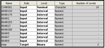
In the following example, I show that the measurement scale of the target variable determines which model is produced by the Regression node. I use the same data that I used in Section 6.2.2, except that I have changed the measurement scale of the target variable $L O S S F R Q$ $L O S S F R Q$ to Nominal. Since the variable $L O S S F R Q$ $L O S S F R Q$ is a discrete version of the continuous variable Loss Frequency, it should be treated as ordinal. I have changed its measurement scale to Nominal only to highlight the fact that the model produced depends on the measurement scale of the target variable.

Display 6.11 shows the flow chart for a regression with a nominal target.

Display 6.11

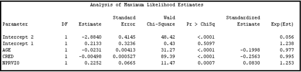
The variables in the data set are set to values identical to the list shown in Display 6.6 with the exception that the measurement scale (level) of the target variable $L O S S F R Q$ $L O S S F R Q$ is set to Nominal. Display 6.12 shows the coefficients of the model estimated by the Regression node.

Display 6.12

Display 6.12 shows that the Regression node has produced two sets of coefficients corresponding to the two equations for calculating the probabilities of the events $L O S S F R Q$ $L O S S F R Q$ =2 and $L O S S F R Q$ $L O S S F R Q$ =1. In contrast to the coefficients shown in Display 6.8, the two equations shown in Display 6.12 have different intercepts and different slopes (i.e., the coefficients of the variables $A G E,$ $A G E,$ $C R E D,$ $C R E D,$ and $N P R V I O$ $N P R V I O$ are also different).

The Regression node gives the following formulas for calculating the probabilities of the events $L O S S F R Q$ $L O S S F R Q$ =2, $L O S S F R Q$ $L O S S F R Q$ =1, and $L O S S F R Q$ $L O S S F R Q$ =0.

$\begin{array}{l} \Pr (L O S S F R Q = 2) = \\ \frac{\exp (1.5946 - 0.0324 * A G E - 0.0134 * C R E D + 0.2186 * N P R V I O)}{1 + \exp (1.5946 - 0.0324 * A G E - 0.0134 * C R E D + 0.2186 * N P R V I O) + \exp (- 0.1186 - 0.0228 * A G E - 0.00449 * C R E D + 0.2240 * N P R V I O)} (6.10) \end{array}$ $\begin{array}{l} \Pr (L O S S F R Q = 2) = \\ \frac{\exp (1.5946 - 0.0324 * A G E - 0.0134 * C R E D + 0.2186 * N P R V I O)}{1 + \exp (1.5946 - 0.0324 * A G E - 0.0134 * C R E D + 0.2186 * N P R V I O) + \exp (- 0.1186 - 0.0228 * A G E - 0.00449 * C R E D + 0.2240 * N P R V I O)} (6.10) \end{array}$

$\begin{array}{l} \Pr (L O S S F R Q = 1) = \\ \frac{\exp (- 0.1186 - 0.0228 * A G E - 0.00449 * C R E D + 0.2240 * N P R V I O)}{1 + \exp (1.5946 - 0.0324 * A G E - 0.0134 * C R E D + 0.2186 * N P R V I O) + \exp (- 0.1186 - 0.0228 * A G E - 0.00449 * C R E D + 0.2240 * N P R V I O)} (6.11) \end{array}$ $\begin{array}{l} \Pr (L O S S F R Q = 1) = \\ \frac{\exp (- 0.1186 - 0.0228 * A G E - 0.00449 * C R E D + 0.2240 * N P R V I O)}{1 + \exp (1.5946 - 0.0324 * A G E - 0.0134 * C R E D + 0.2186 * N P R V I O) + \exp (- 0.1186 - 0.0228 * A G E - 0.00449 * C R E D + 0.2240 * N P R V I O)} (6.11) \end{array}$

\begin{array}{l} \Pr (L O S S F R Q = 0) = \\ \frac{1}{1 + \exp (1.5946 - 0.0324 * A G E - 0.0134 * C R E D + 0.2186 * N P R V I O) + \exp (- 0.1186 - 0.0228 * A G E - 0.00449 * C R E D + 0.2240 * N P R V I O)} (6.12) \end{array}

$\begin{array}{l} \Pr (L O S S F R Q = 0) = \\ \frac{1}{1 + \exp (1.5946 - 0.0324 * A G E - 0.0134 * C R E D + 0.2186 * N P R V I O) + \exp (- 0.1186 - 0.0228 * A G E - 0.00449 * C R E D + 0.2240 * N P R V I O)} (6.12) \end{array}$

Equation 6.12 implies that

$\Pr (L O S S F R Q = 0) = 1 - \Pr (L O S S F R Q = 1) - \Pr (L O S S F R Q = 2) (6.13)$ $\Pr (L O S S F R Q = 0) = 1 - \Pr (L O S S F R Q = 1) - \Pr (L O S S F R Q = 2) (6.13)$

You can check the SAS code produced by the Regression node to verify that the model produced by the Regression node is the same as Equations 6.10, 6.11, 6.12, and 6.13.

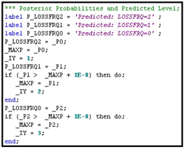
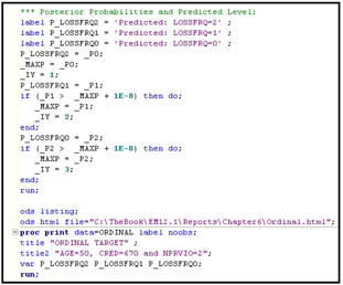
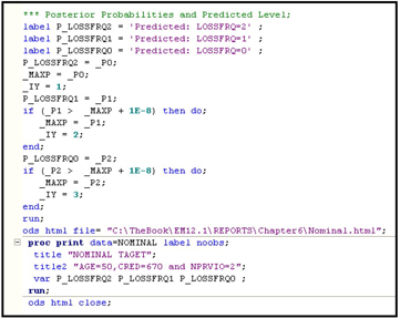
In the results window, click on View → Scoring→SAS Code to see the SAS code generated by the Regression Node. Displays 6.13A and 6.13B show segments of this code.

Display 6.13A

Display 6.13B

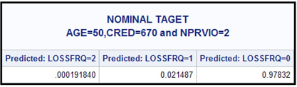
By setting Age=50, CRED=670, and NPRVIO=2, and by using the statements shown in Displays 6.13A and 6.13B, I generated the probabilities that $L O S S F R Q$ $L O S S F R Q$ =0, 1, and 2, as shown in Display 6.14. The SAS code executed for generating these probabilities is given in Displays 6.79 and 6.80 in the appendix to this chapter.

Display 6.14

6.2.4 Models with Continuous Targets

When the target is continuous, the Regression node estimates a linear equation (linear in parameters). The score function is $E (Y / X) = β^{'} X$ $E (Y / X) = β^{'} X$ , where $Y$ $Y$ is the target variable (such as expenditure, income, savings, etc.), $X$ $X$ is a vector of inputs (explanatory variables), and $β$ $β$ is the vector of coefficients estimated by the Regression node.

6.3 An Overview of Some Properties of the Regression Node

A clear understanding of Regression Type, Link Function, Selection Model, and Selection Model Criterion properties is essential for developing predictive models.

In this section, I present a description of these properties in detail.

6.3.1 Regression Type Property

The choices available for this property are Logistic Regression and Linear Regression.

6.3.1.1 Logistic Regression

If your target is categorical (binary, ordinal, or nominal), Logistic Regression is the default regression type. If the target is binary (either numeric or character), the Regression node gives you a Logistic Regression with logit link by default. If the target is categorical with more than two categories, and if its measurement scale (referred to as level in the Variables table of the Input Data Source node) is declared as ordinal, the Regression node by default gives you a model based on a cumulative logits link, as shown in Section 6.2.2. If the target has more than two categories, and if its measurement scale is set to Nominal, then the Regression node gives, by default, a model with a generalized logits link, as shown in Section 6.2.3.

6.3.1.2 Linear Regression

If your target is continuous or if its measurement scale is interval, then the Regression node gives you an ordinary least squares regression by default. A unit link function is used.

6.3.2 Link Function Property

In this section, I discuss various values to which you can set the Link Function property and how the Regression node calculates the predictions of the target for each value of the Link Function property. I start with an explanation of the theory behind the logit and probit link functions for a binary target. You may skip the theoretical explanation and go directly to the formula that the Regression node uses for calculating the target for each specified value of the Link Function property.

I start with the example of a response model, where the target variable takes one of the two values, response and non-response (1 and 0, respectively).

Assume that there is a latent variable $y^{*}$ $y^{*}$ for each record or customer in the data set. Now assume that if the value of $y^{*}$ $y^{*}$ >0, then the customer responds. The value of $y^{*}$ $y^{*}$ depends on the customer’s characteristics as represented by the inputs or explanatory variables, which I can denote by the vector $x$ $x$ . Assume that

y^{*} = β^{'} x + U (6.14)

$y^{*} = β^{'} x + U (6.14)$

where $β$ $β$ is the vector of coefficients and $U$ $U$ is a random variable. Different assumptions about the distribution of the random variable $U$ $U$ give rise to different link functions. I will show how this is so.

The probability of response is

\Pr (y = 1 | x) = \Pr (y^{*} > 0 | x) = \Pr (β^{'} x + U > 0) = \Pr (U > - β^{'} x) (6.15)

$\Pr (y = 1 | x) = \Pr (y^{*} > 0 | x) = \Pr (β^{'} x + U > 0) = \Pr (U > - β^{'} x) (6.15)$

where $y$ $y$ is the target variable.

Therefore,

\Pr (y = 1 | x) = \Pr (U > - β^{'} x) = 1 - F (- β^{'} x) (6.16)

$\Pr (y = 1 | x) = \Pr (U > - β^{'} x) = 1 - F (- β^{'} x) (6.16)$

where $F (.)$ $F (.)$ is the Cumulative Distribution Function (CDF) of the random variable U.

6.3.2.1 Logit Link

If I choose the Logit value for the Link Function property, then the CDF above takes on the following value:

$F (- β^{'} x) = \frac{1}{1 + e^{β^{'} x}}$ $F (- β^{'} x) = \frac{1}{1 + e^{β^{'} x}}$ and $1 - F (- β^{'} x) = 1 - \frac{1}{1 + e^{β^{'} x}} = \frac{1}{1 + e^{- β^{'} x}} (6.17)$ $1 - F (- β^{'} x) = 1 - \frac{1}{1 + e^{β^{'} x}} = \frac{1}{1 + e^{- β^{'} x}} (6.17)$

Hence, the probability of response is calculated as

\Pr (y = 1 | x) = \frac{1}{1 + e^{- β^{'} x}} = \frac{e^{β^{'} x}}{1 + e^{β^{'} x}} (6.18)

$\Pr (y = 1 | x) = \frac{1}{1 + e^{- β^{'} x}} = \frac{e^{β^{'} x}}{1 + e^{β^{'} x}} (6.18)$

From Equation 6.18 you can see that the link function is

\log (\frac{\Pr (y = 1 | x)}{1 - \Pr (y = 1 | x)}) = β^{'} x . (6.19)

$\log (\frac{\Pr (y = 1 | x)}{1 - \Pr (y = 1 | x)}) = β^{'} x . (6.19)$

$β^{'} x$ $β^{'} x$ is called a linear predictor since it is a linear combination of the inputs.

The Regression node estimates the linear predictor and then applies Equation 6.18 to get the probability of response.

6.3.2.2 Probit Link

If I choose the Probit value for the Link Function property, then it is assumed that the random variable $U$ $U$ in Equation 6.14 has a normal distribution with mean=0 and standard deviation=1. In this case I have

\Pr (y = 1 | x) = 1 - F (- β^{'} x) = F (β^{'} x) (6.20)

$\Pr (y = 1 | x) = 1 - F (- β^{'} x) = F (β^{'} x) (6.20)$

where $F (β^{'} x)$ $F (β^{'} x)$ = $\int_{- \infty}^{β^{'} x} \frac{1}{\sqrt{2 π}} e^{- u^{2}} d u (6.21)$ $\int_{- \infty}^{β^{'} x} \frac{1}{\sqrt{2 π}} e^{- u^{2}} d u (6.21)$ .

To estimate the probability of response, the Regression node uses the $p r o b n o r m$ $p r o b n o r m$ function to calculate the probability in Equation 6.20. Thus, it calculates the probability that y=1 as

$\Pr (y = 1 | x) = p r o b n o r m (β^{'} x),$ $\Pr (y = 1 | x) = p r o b n o r m (β^{'} x),$ where the $p r o b n o r m$ $p r o b n o r m$ function gives $F (β^{'} x)$ $F (β^{'} x)$ .

6.3.2.3 Complementary Log-Log Link (Cloglog)

In this case, the Regression node calculates the probability of response as

\Pr (y = 1 | x) = 1 - \exp (- \exp (β^{'} x)) (6.22)

$\Pr (y = 1 | x) = 1 - \exp (- \exp (β^{'} x)) (6.22)$

which is the cumulative extreme value distribution.

6.3.2.4 Identity Link

When the target is interval-scaled, the Regression node uses an identity link. This means that the predicted value of the target variable is equal to the linear predictor $β^{'} x$ $β^{'} x$ . As a result, the predicted value of the target variable is not restricted to the range 0 to 1.

6.3.3 Selection Model Property

The value of this property determines the model selection method used for selecting the variables for inclusion in a regression, whether it is a logistic or linear regression. You can set the value of this property to None, Backward, Forward, or Stepwise.

If you set the value to None, all inputs (sometimes referred to as effects) are included in the model, and there is only one step in the model selection process.

6.3.3.1 Backward Elimination Method

To use this method, set the Selection Model property to Backward, set the Use Selection Defaults property to No, and set the Stay Significance Level property to a desired threshold level of significance (such as 0.025, 0.05, 0.10, etc.) by opening the Selection Options window. Also, set the Maximum Number of Steps to a value such as 100 in the Selection Options window..

In this method, the process of model fitting starts with Step 0, where all inputs are included in the model. For each parameter estimated, a Wald Chi-Square test statistic is computed. In Step 1, the input whose coefficient is least significant and that also does not meet the threshold set by Stay Significance Level property in the Selection Options group (i.e., the p-value of its Chi-Square test statistic is greater than the value to which the Stay Significance Level property is set) is removed. Also, from the remaining variables, a new model is estimated and a Wald Chi-Square test statistic is computed for the coefficient of each input in the estimated model. In Step 2, the input whose coefficient is least significant (and that does not meet the Stay Significance Level threshold) is removed, and a new model is built. This process is repeated until no more variables fail to meet the threshold specified. Once a variable is removed at any step, it does not enter the equation again.

If this selection process takes ten steps (including Step 0) before it comes to a stop, then ten models are available when the process stops. From these ten models, the Regression node selects one model. The criterion used for the selection of a final model is determined by the value to which the Selection Criterion property is set. If the Selection Criterion property is set to None, then the final model selected is the one from the last step of the Backward Elimination process. If the Selection Criterion property is set to any value other than None, then the Regression node uses the criterion specified by the value of the Selection Criterion property to select the final model. Alternative values of the Selection Criterion property and a description of the procedures the Regression node follows to select the final model according to each of these criteria are discussed in Section 6.3.4.

6.3.3.1A Backward Elimination Method When the Target Is Binary

To demonstrate the backward selection method, I use a data set with only ten inputs and a binary target. Display 6.15 shows the process flow diagram for this demonstration.

Display 6.15

To demonstrate the backward selection method I used a data set with only ten inputs and a binary target shown in Display 6.16

Display 6.16

Display 6.17 shows the property settings of the Regression node in the process flow shown in Display 6.15.

Display 6.17

By setting the Use Selection Defaults properties to Yes, the value of the Stay Significance Level property is set to 0.05 by default. When the Stay Significance Level property is set to 0.05, the Regression node eliminates variables with a p-value greater than 0.05 in the backward elimination process. You can set the Stay Significance Level property to a value different from the default value of 0.05 by setting the Use Selection Defaults property to No, and then opening the Selection Options window by clicking next to the Selection Options property.

Display 6.18 shows the Selection Options window.

Display 6.18

Displays 6.19A, 6.19B, and 6.19C illustrate the backward selection method.

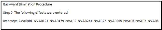
Display 6.19A shows that at Step 0, all of the ten inputs are included in the model.

Display 6.19A

Display 6.19B shows that in Step 1, the variable NVAR5 was removed because its Wald Chi-Square Statistic had the highest p-value (0.8540) (which is above the threshold significance level of 0.05 specified in the Stay Significance Level property). Next, a model with only nine inputs (all except NVAR5) was estimated, and a Wald Chi-Square statistic was computed for the coefficient of each input. Of the remaining variables, NVAR8 had the highest p-value for the Wald Test statistic, and so this input was removed in Step 2 and a logistic regression was estimated with the remaining eight inputs. This process of elimination continued until two more variables, NVAR2 and NVAR179, were removed at Steps 3 and 4 respectively.

Display 6.19B

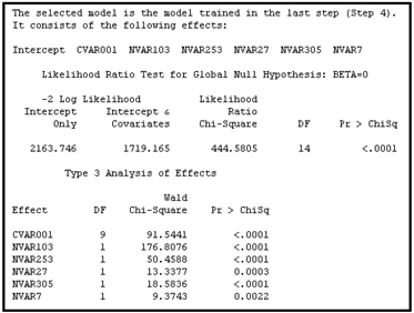
The Wald Test statistic was then computed for the coefficient of each input included in the model. At this stage, none of the p-values were above the threshold value of 0.05. Hence, the final model is the model developed at the last step, namely Step 4. Display 6.19C shows the variables included in the final model and shows that the p-values for all the included inputs are below the Stay Significance Level property value of 0.05.

Display 6.19C

6.3.3.1B Backward Elimination Method When the Target Is Continuous

The backward elimination method for a continuous target is similar to that for a binary target. However, when the target is continuous, an F statistic is used instead of Wald Chi-Square statistic for calculating the p-values.

To demonstrate the backward elimination property for a continuous target, I used the process flow shown Display 6.20.

Display 6.20

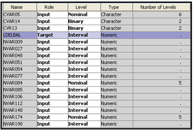
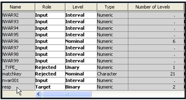
As shown in Display 6.21, there are sixteen inputs in the modeling data set used in this example.

Display 6.21

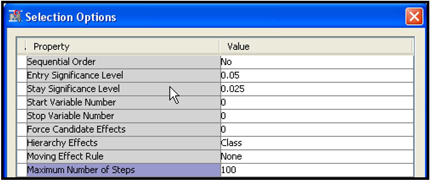
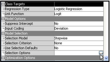
Display 6.22 shows the properties of the Regression node in the process flow shown in Display 6.20.

Display 6.22

Open the Selection Options window (shown in Display 2.23) by clicking .

Display 6.23

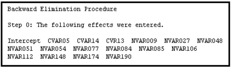
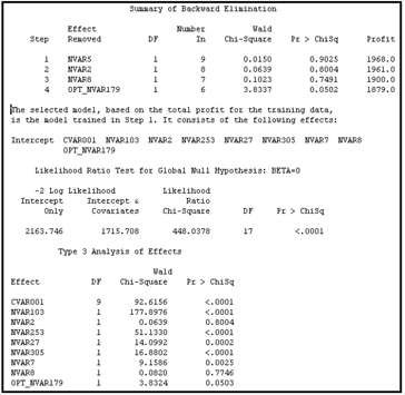
In Step 0 (See Display 6.24A), all 16 inputs were included in the model.

Display 6.24A

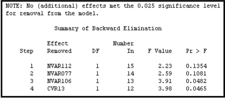
In the backward elimination process, four inputs were removed, one at each step. These results are shown in Display 6.24B.

Display 6.24B

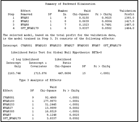
Display 6.24C shows inputs included in the final model.

Display 6.24C

Display 6.24C shows the variables included in the final model, along with the F statistics and p-values for the variable coefficients. The F statistics are partial F’s since they are adjusted for the other effects already included in the model. In other words, the F statistic shown for each variable is based on a partial sum of squares, which measures the increase in the model sum of squares due to the addition of the variable to a model that already contains all the other main effects (11 in this case) plus any interaction terms (0 in this case). This type of analysis, where the contribution of each variable is adjusted for all other effects including the interaction effects, is called a Type 3 analysis.

At this point, it may be worth mentioning Type 2 sum of squares. According to Littell, Freund, and Spector, “Type 2 sum of squares for a particular variable is the increase in Model sum of square due to adding the variable to a model that already contains all other variables. If the model contains only main effects, then type 3 and type 2 analyses are the same.”² For a discussion of partial sums of squares and different types of analysis, see SAS System for Linear Models.³

6.3.3.2 Forward Selection Method

To use this method, set the Selection Model property to Forward, set the Use Selection Default property to No, and set the Entry Significance Level property to a desired threshold level of significance, such as 0.025 0.05, etc.

6.3.3.2A Forward Selection Method When the Target Is Binary

At Step 0 of the forward selection process, the model consists of only the intercept and no other inputs. At the beginning of Step 1, the Regression node calculates the score Chi-Square statistic⁴ for each variable not included in the model and selects the variable with the largest score statistic, provided that it also meets the Entry Significance Level threshold value. At the end of Step 1, the model consists of the intercept plus the first variable selected. In Step 2, the Regression node again calculates the score Chi-Square statistic for each variable not included in the model and similarly selects the best variable. This process is repeated until none of the remaining variables meets the Entry Significance Level threshold. Once a variable is entered into the model at any step, it is never removed.

To demonstrate the Forward Selection method, I used a data set with a binary target. The process flow diagram for this demonstration is shown in Display 6.25.

Display 6.25

In the Regression node, I set the Selection Model property to Forward, the Entry Significance Level property to 0.025, and the Selection Criterion property to None. Displays 6.26A, 6.26B, and 6.26C show how the Forward Selection method works when the target is binary.

Display 6.26A

Display 6.26B

Display 6.26C

Display 6.26C shows that twelve of the sixteen variables in the final model have p-values below the threshold level of 0.025. These variables were significant when they entered the equation (see Display 6.26B), and remained significant even after other variables entered the equation at the subsequent steps. However, the variables IMP_NVAR177, IMP_NVAR215, IMP_NVAR305, and IMP_NVAR304 were significant when they entered the equation (see Display 6.26B), but they became insignificant (their p-values are greater than 0.025) in the final model. You should examine these variables and determine whether they are collinear with other variables, have a highly skewed distribution, or both.

6.3.3.2B Forward Selection Method When the Target Is Continuous

Once again, at Step 0 of the forward selection process, the model consists only of the intercept. At Step 1, the Regression node calculates, for each variable not included in the model, the reduction in the sum of squared residuals that would result if that variable were included in the model. It then selects the variable that, when added to the model, results in the largest reduction in the sum of squared residuals, provided that the p-value of the F statistic for the variable is less than or equal to the Entry Significance Level threshold. At Step 2, the variable selected in Step 1 is added to the model, and the Regression node again calculates, for each variable not included in the model, the reduction in the sum of squared residuals that would result if that variable were included in the model. Again, the variable whose inclusion results in the largest reduction in the sum of squared residuals is added to the model, and so on, until none of the remaining variables meets the Entry Significance Level threshold value. As with the binary target, once a variable is entered into the model at any step, it is never removed.

Display 6.27 shows the process flow created for demonstrating the Forward Selection method when the target is continuous.

Display 6.27

The target variable in the Input Data shown in Display 6.27 is continuous. In the Regression node, I set the Regression Type property to Linear Regression, the Selection Model property to Forward, the Selection Criterion property to None, and the Use Selection Defaults property to Yes. The Entry Significance Level property is set to its default value of 0.05.

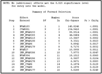
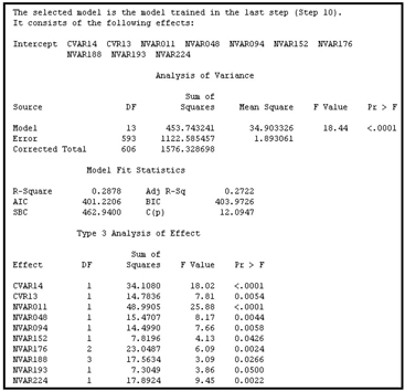
Displays 6.28A, 6.28B and 6.28C show how the Forward Selection method works when the target is continuous.

Display 6.28A

Display 6.28B

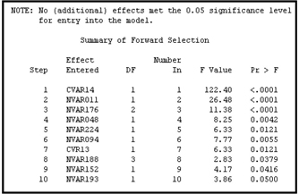
Display 6.28C

6.3.3.3 Stepwise Selection Method

To use this method, set the Selection Model property to Stepwise, the Selection Default property to No, the Entry Significance Level property to a desired threshold level of significance (such as 0.025, 0.05, 0.1, etc.) and the Stay Significance Level to a desired value (such as 0.025, 0.05, etc.).

The stepwise selection procedure consists of both forward and backward steps, although the backward steps may or may not yield any change in the forward path. The variable selection is similar to the forward selection method except that the variables already in the model do not necessarily remain in the model. When a new variable is entered at any step, some or all variables that are already included in the model may become insignificant. Such variables may be removed by the same procedures used in the backward method. Thus, variables are entered by forward steps and removed by backward steps. A forward step may be followed by more than one backward step.

6.3.3.3A Stepwise Selection Method When the Target Is Binary

Display 6.29 shows the process flow used for demonstrating the Stepwise Selection method.

Display 6.29

Display 6.30 shows a partial list of the variables in the input data set RESP_SMPL_CLEAN4_C.

Display 6.30

As shown in Display 6.30, the target variable RESP is binary. Display 6.31 shows the property settings of the Regression node.

Display 6.31

Display 6.32 shows the Selection Options properties.

Display 6.32

The results are shown in Displays 6.33A, 6.33B, and 6.33C.

Display 6.33A

Display 6.33B

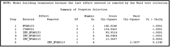
Display 6.33C

Comparing the variables shown in Display 6.33C with those shown in Display 6.26C, you can see that the stepwise selection method produced a slightly more parsimonious (and therefore better) solution than the forward selection method. The forward selection method selected 16 variables (Display 6.26C), while the stepwise selection method selected 4 variables.

6.3.3.3B Stepwise Selection Method When the Target Is Continuous

The stepwise procedure in the case of a continuous target is similar to the stepwise procedure used when the target is binary. In the forward step, the R-square, along with the F statistic, is used to evaluate the input variables. In the backward step, partial F statistics are used.

Display 6.34 shows the process flow for demonstrating the Stepwise Selection method when the target is continuous.

Display 6.34

Display 6.35 shows a partial list of variables included in the Input data set in the process flow diagram shown in Display 6.34.

Display 6.35

Display 6.36 shows the property settings of the Regression node used in this demonstration.

Display 6.36

In the Selection Options window, I set the Entry Significance Level property to 0.1, the Stay Significance Level property to 0.025, and the Maximum Number of Steps property to 100.

The results are shown in Displays 6.37A, 6.37B, and 6.37C.

Display 6.37A

Display 6.37B

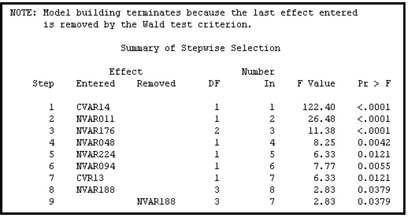
Display 6.37C

6.3.4 Selection Criterion Property⁵

In Section 6.3.3, I pointed out that during the backward, forward, and stepwise selection methods, the Regression node creates one model at each step. When you use any of these selection methods, the Regression node selects the final model based on the value to which the Selection Criterion property is set. If the Selection Criterion property is set to None, then the final model is simply the one created in the last step of the selection process. But any value other than None requires the Regression node to use the criterion specified by the value of the Selection Criterion property to select the final model.

You can set the value of the Selection Criterion property to any one of the following options:

• Akaike Information Criterion (AIC)

• Schwarz Bayesian Criterion (SBC)

• Validation Error

• Validation Misclassification

• Cross Validation Error

• Cross Validation Misclassification

• Validation Profit/Loss

• Profit/Loss

• Cross Validation Profit/Loss

• None

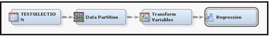
In this section, I demonstrate how these criteria work by using a small data set TestSelection, as shown in Display 6.38.

Display 6.38

For all of the examples shown in this section, in the Properties panel, I set the Regression Type property to Logistic Regression, the Link Function property to Logit, the Selection Model property to Backward, the Stay Significance Level property to 0.05, and the Selection Criterion property to one of the values listed above.

The Selection Options properties are shown in Display 6.39.

Display 6.39

To understand the Akaike Information Criterion and the Schwarz Bayesian Criterion, it is helpful to first review the computation of the errors in models with binary targets (such as response to a direct mail marketing campaign).

Let $\hat{π} (x_{i})$ $\hat{π} (x_{i})$ represent the predicted probability of response for the $i^{t h}$ $i^{t h}$ record, where $x_{i}$ $x_{i}$ is the vector of inputs for the $i^{t h}$ $i^{t h}$ customer record. Let $y_{i}$ $y_{i}$ represent the actual outcome for the $i^{t h}$ $i^{t h}$ record, where $y_{i}$ $y_{i}$ =1 if the customer responded and $y_{i}$ $y_{i}$ =0 otherwise. For a responder, the error is measured as the difference between the log of the actual value for $y_{i}$ $y_{i}$ and the log of the predicted probability of response ( $\hat{π} (x_{i})$ $\hat{π} (x_{i})$ ). Since $y_{i}$ $y_{i}$ =1,

E r r o r =_{i} \log (\frac{y_{i}}{\hat{π} (x_{i})}) = - \log (\frac{\hat{π} (x_{i})}{y_{i}}) = - y_{i} \log (\frac{\hat{π} (x_{i})}{y_{i}}).

$E r r o r =_{i} \log (\frac{y_{i}}{\hat{π} (x_{i})}) = - \log (\frac{\hat{π} (x_{i})}{y_{i}}) = - y_{i} \log (\frac{\hat{π} (x_{i})}{y_{i}}).$

For a non-responder the error is represented as

E r r o r_{i} = - (1 - y_{i}) \log (\frac{1 - \hat{π} (x_{i})}{1 - y_{i}}) .

$E r r o r_{i} = - (1 - y_{i}) \log (\frac{1 - \hat{π} (x_{i})}{1 - y_{i}}) .$

Combining both the response and non-response possible outcomes, the error for the $i^{t h}$ $i^{t h}$ customer record can be represented by

E r r o r_{i} = - [y_{i} \log (\frac{{\hat{π}}_{i} (x_{i})}{y_{i}}) + (1 - y_{i}) \log (\frac{1 - {\hat{π}}_{i} (x_{i})}{1 - y_{i}})] .

$E r r o r_{i} = - [y_{i} \log (\frac{{\hat{π}}_{i} (x_{i})}{y_{i}}) + (1 - y_{i}) \log (\frac{1 - {\hat{π}}_{i} (x_{i})}{1 - y_{i}})] .$

Notice that the second term in the brackets goes to zero in the case of a responder. Hence, the first term gives the value of the error in that case. And in the case of a non-responder, the first term goes to zero and the error is given by the second term alone.

Summing the errors for all the records in the data set, I get

E r r o r S u m = - \sum_{i = 1}^{n} [y_{i} \log (\frac{{\hat{π}}_{i} (x_{i})}{y_{i}}) + (1 - y_{i}) \log (\frac{1 - {\hat{π}}_{i} (x_{i})}{1 - y_{i}})] (6.23)

$E r r o r S u m = - \sum_{i = 1}^{n} [y_{i} \log (\frac{{\hat{π}}_{i} (x_{i})}{y_{i}}) + (1 - y_{i}) \log (\frac{1 - {\hat{π}}_{i} (x_{i})}{1 - y_{i}})] (6.23)$

where $n$ $n$ is the number of records in the data set.

In general, Equation 6.23 is used as the measure of model error for models with a binary target. By taking the anti-logs of Equation 6.23, we get

- \prod_{i = 1}^{n} \frac{{({\hat{π}}_{i} (x_{i}))}^{y_{i}}}{y_{i}^{y_{i}}} \frac{{(1 - {\hat{π}}_{i} (x_{i}))}^{^{1 - y_{i}}}}{{(1 - y_{i})}^{1 - y_{i}}} (6.24)

$- \prod_{i = 1}^{n} \frac{{({\hat{π}}_{i} (x_{i}))}^{y_{i}}}{y_{i}^{y_{i}}} \frac{{(1 - {\hat{π}}_{i} (x_{i}))}^{^{1 - y_{i}}}}{{(1 - y_{i})}^{1 - y_{i}}} (6.24)$

which can be rewritten as

- \frac{\prod_{i = 1}^{n} {({\hat{π}}_{i} (x_{i}))}^{y_{i}} {(1 - {\hat{π}}_{i} (x_{i}))}^{1 - y_{i}}}{\prod_{i = 1}^{n} y_{i}^{y_{i}} {(1 - y_{i})}^{1 - y_{i}}} (6.25)

$- \frac{\prod_{i = 1}^{n} {({\hat{π}}_{i} (x_{i}))}^{y_{i}} {(1 - {\hat{π}}_{i} (x_{i}))}^{1 - y_{i}}}{\prod_{i = 1}^{n} y_{i}^{y_{i}} {(1 - y_{i})}^{1 - y_{i}}} (6.25)$

The denominator of Equation 6.25 is 1, and the numerator is simply the likelihood of the model, often represented by the symbol $L$ $L$ , so I can write

- \prod_{i = 1}^{n} {({\hat{π}}_{i} (x_{i}))}^{y_{i}} {(1 - {\hat{π}}_{i} (x_{i}))}^{1 - y_{i}} = - L (6.26)

$- \prod_{i = 1}^{n} {({\hat{π}}_{i} (x_{i}))}^{y_{i}} {(1 - {\hat{π}}_{i} (x_{i}))}^{1 - y_{i}} = - L (6.26)$

Taking logs of the terms on both sides in Equation 6.27, I get

- L o g L = - \sum_{i = 1}^{n} [y_{i} \log ({\hat{π}}_{i} (x_{i})) + (1 - y_{i}) \log (1 - {\hat{π}}_{i} (x_{i}))] (6.27)

$- L o g L = - \sum_{i = 1}^{n} [y_{i} \log ({\hat{π}}_{i} (x_{i})) + (1 - y_{i}) \log (1 - {\hat{π}}_{i} (x_{i}))] (6.27)$

The expression given in Equation 6.27 is multiplied by 2 to obtain a quantity with a known distribution, giving the expression

- 2 L o g L = - 2 \sum_{i = 1}^{n} [y_{i} \log ({\hat{π}}_{i} (x_{i})) + (1 - y_{i}) \log (1 - {\hat{π}}_{i} (x_{i}))] (6.28)

$- 2 L o g L = - 2 \sum_{i = 1}^{n} [y_{i} \log ({\hat{π}}_{i} (x_{i})) + (1 - y_{i}) \log (1 - {\hat{π}}_{i} (x_{i}))] (6.28)$

The quantity shown in Equation 6.28 is used as a measure of model error for comparing models when the target is binary.

In the case of a continuous target, the model error is the sum of the squares of the errors of all the individual records of the data set, where the errors are the simple differences between the actual and predicted values.

6.3.4.1 Akaike Information Criterion (AIC)

When used for comparing different models, the Akaike Information Criterion (AIC) adjusts the quantity shown in Equation 6.28 in the following way.

The Akaike Information Criterion (AIC) statistic is

A I C = - 2 L o g L + 2 (k + s) (6.29)

$A I C = - 2 L o g L + 2 (k + s) (6.29)$

where $k$ $k$ is the number of response levels minus 1, and $s$ $s$ is the number of explanatory variables in the model. The AIC statistic has two parts. The first part is $- 2 L o g L$ $- 2 L o g L$ , which is a measure of model error, and it tends to decrease as we add more explanatory variables to the model. The second part $2 (k + s)$ $2 (k + s)$ can be considered as a penalty term that depends on the number of explanatory variables included in the model. It increases with the number of explanatory variables added to the model. Inclusion of the penalty term is to reduce the chances of including too many explanatory variables, which may lead to over- fitting.

When I performed a model selection on my example data set (using backward elimination) and set the Selection Criterion property to Akaike Information Criterion, there were four steps in the model selection process. The model from Step 1 was selected since the Akaike Information Criterion statistic was the lowest at step1. Display 6.40 shows the Akaike Information Criterion Statistic at each step of the iteration.

Display 6.40

Displays 6.41 shows the Backward Elimination process and Display 6.42 shows the variables in the selected model.

Display 6.41

Display 6.42

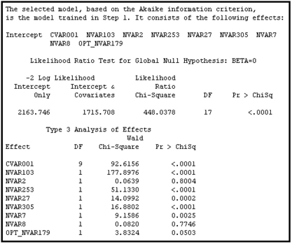
You can see in Display 6.41 that the model created in Step 1 has the smallest value of AIC statistic. However, as you can see from Display 6.42, the selected model (created in Step 1) includes two variables (NVAR2 and NVAR8) that are not significant or have a high p-value. You can avoid this type of situation by eliminating (or combining) collinear variables from the data set before running the Regression node. You can use the Variable Clustering node, discussed in Chapter 2, to identify redundant/related variables.

6.3.4.2 Schwarz Bayesian Criterion (SBC)

The Schwarz Bayesian Criterion (SBC) adjusts $- 2 L o g L$ $- 2 L o g L$ in the following way:

S B C = - 2 L o g L + (k + s) n (6.30)

$S B C = - 2 L o g L + (k + s) n (6.30)$

where k and s are same as in Equation 6.29 and $n$ $n$ is the number of observations.

Like the AIC statistic, the SBC statistic also has two parts. The first part is $- 2 L o g L$ $- 2 L o g L$ , which a measure of model error, and the second part is the penalty term $(k + s) n$ $(k + s) n$ . The penalty for including additional variables is higher in SBC statistic than in AIC statistic.

When the Schwarz Bayesian Criterion is used, the Regression node selects the model with the smallest value for the Schwarz Bayesian Criterion statistic.

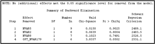
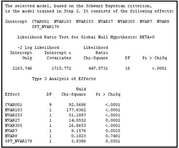
As Displays 6.43 and 6.44 show, the model selection process again took only four steps, but this time the model from Step 2 is selected.

Display 6.43 shows a plot of the SBC statistic at each step in the backward elimination process.

Display 6.43

Display 6.44 shows the variables removed at successive steps of backward elimination process.

Display 6.44

Display 6.45 shows the variables included in the selected model.

Display 6.45

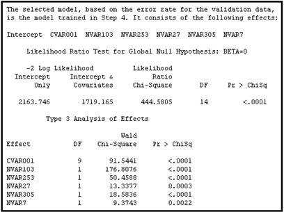
6.3.4.3 Validation Error

In the case of a binary target, validation error is the error calculated by the negative log likelihood expression shown in Equation 6.28. The error is calculated from the Validation data set for each of the models generated at the various steps of the selection process. The parameters of each model are used to calculate the predicted probability of response for each record in the data set. In Equation 6.28 this is shown as $\hat{π} (x_{i})$ $\hat{π} (x_{i})$ , where $x_{i}$ $x_{i}$ is the vector of inputs for the $i^{t h}$ $i^{t h}$ record in the Validation data set. (In the case of a continuous target, the validation error is the sum of the squares of the errors calculated from the Validation data set, where the errors are the simple differences between the actual and predicted values for the continuous target.) The model with the smallest validation error is selected, as shown in Displays 6.46 and 6.47.

Display 6.46

Display 6.47

6.3.4.4 Validation Misclassification

For analyses with a binary target such as response, a record in the Validation data set is classified as a responder if the posterior probability of response is greater than the posterior probability of non-response. Similarly, if the posterior probability of non-response is greater than the posterior probability of response, the record is classified as a non-responder. These posterior probabilities are calculated for each customer in the Validation data set using the parameters estimated for each model generated at each step of the model-selection process. Since the validation data includes the actual customer response for each record, you can check whether the classification is correct or not. If a responder is correctly classified as a responder, or a non-responder is correctly classified as a non-responder, then there is no misclassification; otherwise, there is a misclassification. The error rate for each model can be calculated by dividing the total number of misclassifications in the validation data set by the total number of records. The validation misclassification rate is calculated for each model generated at the various steps of the selection process, and the model with the smallest validation misclassification rate is selected.

Display 6.48 shows the model selected by the Validation Misclassification criterion.

Display 6.48

6.3.4.5 Cross Validation Error

In SAS Enterprise Miner, cross validation errors are calculated from the Training data set. One observation is omitted at a time, and the model is re-estimated with the remaining observations. The re-estimated model is then used to predict the value of the target for the omitted observation, and then the error of the prediction, in the case of a binary target, is calculated using the formula given in Equation 6.28 with $n$ $n$ =1. (In the case of a continuous target, the error is the squared difference between the actual and predicted values.) Next, another observation is omitted, the model is re-estimated and used to predict the omitted observation, and this new prediction error is calculated. This process is repeated for each observation in the Training data set, and the aggregate error is found by summing the individual errors.

If you do not have enough observations for training and validation, then you can select the Cross Validation Error criterion for model selection. The data sets I used have several thousand observations. Therefore, in my example, it may take a long time to calculate the cross validation errors, especially since there are several models. Hence this criterion is not tested here.

6.3.4.6 Cross Validation Misclassification Rate

The cross validation misclassification rate is also calculated from the Training data set. As in the case described in Section 6.3.4.5, one observation is omitted at a time, and the model is re-estimated every time. The re-estimated model is used to calculate the posterior probability of response for the omitted observation. The observation is then assigned a target level (such as response or non-response) based on maximum posterior probability. SAS Enterprise Miner then checks the actual response of the omitted customer to see if this re-estimated model misclassifies the omitted customer. This process is repeated for each of the observations, after which the misclassifications are counted, and the misclassification rate is calculated. For the same reason cited in Section 6.3.4.5, I have not tested this criterion.

6.3.4.7 The Validation Profit/Loss Criterion

In order to use the Validation Profit/Loss criterion, you must provide SAS Enterprise Miner with a profit matrix. To demonstrate this method, I have provided the profit matrix shown in Display 6.49.

Display 6.49

When calculating the profit/loss associated with a given model, the Validation data set is used. From each model produced by the backward elimination process, a formula for calculating posterior probabilities of response and non-response is generated in this example. Using these posterior probabilities, the expected profits under Decision1 (assigning the record to the responder category) and Decision2 (assigning the record to the non-responder category) are calculated. If the expected profit under Decision1 is greater than the expected profit under Decision2, then the record is assigned the target level responder; otherwise, it is set to non-responder. Thus, each record in the validation data set is assigned to a target level.

The following equations show how the expected profit is calculated, given the posterior probabilities calculated from a model and the profit matrix shown in Display 6.49.

The expected profit under Decision1 is

E_{1 i} = $ 10 * \hat{π} (x_{i}) + (- $ 1) (1 - \hat{π} (x_{i})) (6.31)

$E_{1 i} = $ 10 * \hat{π} (x_{i}) + (- $ 1) (1 - \hat{π} (x_{i})) (6.31)$

where $E_{1 i}$ $E_{1 i}$ is the expected profit under Decision1 for the $i^{t h}$ $i^{t h}$ record, $\hat{π} (x_{i})$ $\hat{π} (x_{i})$ is the posterior probability of response of the $i^{t h}$ $i^{t h}$ record, and $x_{i}$ $x_{i}$ is the vector of inputs for the $i^{t h}$ $i^{t h}$ record in the validation data set.

The expected profit under Decision2 (assigning the record to the target level non-responder) is

E_{2 i} = $ 0 * \hat{π} (x_{i}) + $ 0 (1 - \hat{π} (x_{i})) (6.32)

$E_{2 i} = $ 0 * \hat{π} (x_{i}) + $ 0 (1 - \hat{π} (x_{i})) (6.32)$

which is always zero in this case, given the profit matrix I have chosen.

The rule for classifying customers is:

If $E_{1 i} > E_{2 i}$ $E_{1 i} > E_{2 i}$ , then assign the record to the target level responder. Otherwise, assign the record to the target level non-responder.

Having assigned a target category such as responder or non-responder to each record in the Validation data set, you can examine whether the decision taken is correct by comparing the assignment to the actual value. If a customer record is assigned the target class of responder and the customer is truly a responder, then the company has made a profit of $10. This is the actual profit that I would have made—not the expected profit calculated before. If, on the other hand, we assigned the target class responder and the customer turned out to be a non-responder, then I incur a loss of $1. According to the profit matrix given in Display 6.49, there is no profit or loss if I assigned the target level non-responder to a true responder or a target level of non-responder to a true non-responder. Thus, based on the decision and the actual outcome for each record, I can calculate the actual profit for each customer in the Validation data set. And by summing the profits across all of the observations, I obtain the validation profit/loss. These calculations are made for each model generated at various iterations of the model selection process. The model that yields the highest profit is selected.

Display 6.50 shows the model selected by this criterion for my example problem.

Display 6.50

6.3.4.8 Profit/Loss Criterion

When this criterion is selected, the profit/loss is calculated in the same way as the validation profit/lLoss above, but it is done using the training data set instead of the validation data. Again, you resort to this option only when there is insufficient data to create separate Training and Validation data sets. Display 6.51 shows the results of applying this option to my example data.

Display 6.51

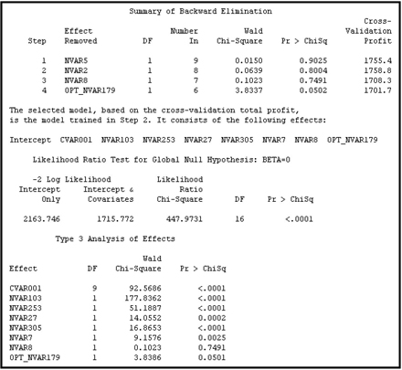
6.3.4.9 The Cross Validation Profit/Loss Criterion

The process by which the Cross Validation Profit/Loss criterion is calculated is similar to the cross validation misclassification rate method described in Section 6.3.4.6. At each step, one observation is omitted, the model is re-estimated, and the re-estimated model is used to calculate posterior probabilities of the target levels (such as response or no-response) for the omitted observation. Based on the posterior probability and the profit matrix that is specified, the omitted observation is assigned a target level in such a way that the expected profit is maximized for that observation, as described in Section 6.3.4.7. Actual profit for the omitted record is calculated by comparing the actual target level and the assigned target level. This process is repeated for all the observations in the data set. By summing the profits across all of the observations, I obtain the cross validation profit/loss. These calculations are made for each model generated at various steps of the model selection process. The model that yields the highest profit is selected. The selected model is shown in Display 6.52

Display 6.52

6.4 Business Applications

The purpose of this section is to illustrate the use of the Regression node with two business applications, one requiring a binary target, and the other a continuous target.

The first application is concerned with identifying the current customers of a hypothetical bank who are most likely to respond to an invitation to sign up for Internet banking that carries a monetary reward with it. A pilot study was already conducted in which a sample of customers were sent the invitation. The task of the modeler is to use the results of the pilot study to develop a predictive model that can be used to score all customers and send mail to those customers who are most likely to respond (a binary target).

The second application is concerned with identifying customers of a hypothetical bank who are likely to increase their savings deposits by the largest dollar amounts if the bank increases the interest paid to them by a preset number of basis points. A sample of customers was tested first. Based on the results of the test, the task of the modeler is to develop a model to use for predicting the amount each customer would increase his savings deposits (a continuous target), given the increase in the interest paid. (Had the test also included several points representing decrease, increase, and no change from the current rate, then the estimated model could be used to test the price sensitivity in any direction. However, in the current study, the bank is interested only in the consequences of a rate increase to customer’s savings deposits.)

Before using the Regression node for modeling, you need to clean the data. This very important step includes purging some variables, imputing missing values, transforming the inputs, and checking for spurious correlation between the inputs and the target. Spurious correlations arise when input variables are derived in part from the target variables, generated from target variable behavior, or are closely related to the target variable. Post-event inputs (inputs recorded after the event being modeled had occurred) might also cause spurious correlations.

I performed a prior examination of the variables using the StatExplore and MultiPlot nodes, and excluded some variables, such as the one shown Displays 6.53, from the data set.

Display 6.53

In Display 6.53, the variable CVAR12 is a categorical input, taking the values Y and N. A look at the distribution of the variable shown in the 2x2 table suggests that it might be derived from the target variable or connected to it somehow, or it might be an input with an uneven spread across the target levels. Variables such as these can produce undesirable results, and they should be excluded from the model if their correlation with the target is truly spurious. However, there is also the possibility that this variable has valuable information for predicting the target. Clearly, only a modeler who knows where his data came from, how the data were constructed, and what each variable represents in terms of the characteristics and behaviors of customers will be able to detect spurious correlations. As a precaution before applying the modeling tool, you should examine every variable included in the final model (at a minimum) for this type of problem.

In order to demonstrate alternative types of transformations, I present three models for each type of target that is discussed. The first model is based on untransformed inputs. This type of model can be used to make a preliminary identification of important inputs. For the second model, the transformations are done by the Transform Variables node, and for the third model transformations are done by the Decision Tree node.

The Transform Variables node has a variety of transformations (discussed in detail in Section 2.9.6 of Chapter 2 and in Section 3.5 of Chapter 3). I use some of these transformation methods here for demonstration purposes.

The transformations produced by the Decision Tree node yield a new categorical variable, and this happens in the following way. First, a Decision Tree model is built based on the inputs in order to predict the target (or classify records). Next, a categorical variable is created, where the value (category) of the variable for a given record is simply the leaf to which the record belongs. The Regression node then uses this categorical variable as a class input. The Regression node creates a dummy variable for each category and uses it in the regression equation. These dummy variables capture the interactions between different inputs included in the tree, which are potentially very important.

If there are a large number of variables, you can use the Variable Selection node to screen important variables prior to using the Regression node. However, since the Regression node itself has several methods of variable selection (as shown in Sections 6.3.3 and 6.3.4), and since a moderate number of inputs is contained in each of my data sets, I did not use the Variable Selection node prior to using the Regression node in these examples.

Two data sets are used in this chapter: one for modeling the binary target and the other for a modeling the continuous target. Both of these are simulated. The results may therefore seem too good to be true at times, and not so good at other times.

6.4.1 Logistic Regression for Predicting Response to a Mail Campaign

For predicting response, I explore three different ways of developing a logistic regression model. The models developed are Model_B1, Model_B2, and Model_B3. The process flow for each model is shown in Display 6.54.

Display 6.54

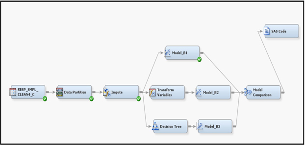
In the process flow, the first node is the Input Data Source node that reads the modeling data. From this modeling data set, the Data Partition node creates three data sets Part_Train, Part_Validate, and Part_Test according to the Training, Validation, and Test properties, which I set at 40%, 30%, and 30%, respectively. These data sets, with the roles of Train, Validate and Test, are passed to the Impute node. In the Impute node, I set the Default Input Method property to Median for the interval variables, and I set it to Count for the class variables. The Impute node creates three data sets Impt_Train, Impt_Validate, and Impt_Test including the imputed variables, and passes them to the next node. The last node in the process flow shown in Display 6.54 is the Model Comparison node. This node generates various measures such as lift, capture rate, etc., from the training, validation, and test data sets.

6.4.1.1 Model_B1

The process flow for Model_B1 is at the top segment of Display 6.54. The Regression node uses the data set Impt_Train for effect selection. Each step of the effects selection method generates a model. The Validation data set is used by the Regression node to select the best model from those generated at several steps of the selection process. Finally, the data set Impt_Test is used to get an independent assessment of the model. This is done in the Model Comparison node at the end of the process flow.

Display 6.55 shows the settings of the Regression node properties for Model_B1.

Display 6.55

By opening the Results window and scrolling through the output, you can see the models created at different steps of the effect selection process and the final model selected from these steps. In this example, the Regression node took six steps to complete the effect selection. The model created at Step 4 is selected as the final model since it minimized the validation error.

Display 6.56 shows the variables included in the final model.

Display 6.56

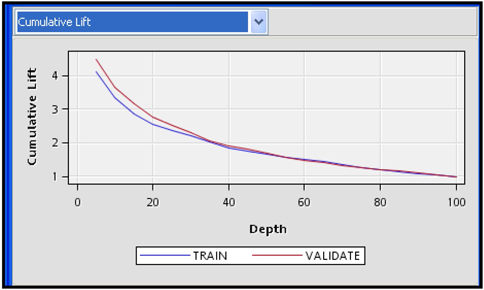
Display 6.56 shows a partial view of the output in the Results window. Display 6.57 shows the lift charts for the final Model_B1. These charts are displayed under Score Rankings Overlay in the Results window.

Display 6.57

If you click anywhere under Score Rankings Overlay in the Results window and select the Table icon, you will see the table shown in Display 6.58.

Display 6.58

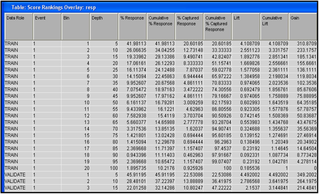
The table shown in Display 6.58 contains several measures such as lift, cumulative lift, capture rate, etc., by percentile for the Training and Validation data sets. This table is saved is a SAS data set, and you can use it for making custom tables such as Table 6.1.

The table shown in Display 6.58 is created by first sorting the Training and Validation data sets individually in descending order of the predicted probability, and dividing each data set into 20 equal sized groups or bins, such that Bin 1 contains 5% records with the highest predicted probability, Bin 2 contains 5% of records with the next highest predicted probability, etc. The measures such as lift, cumulative lift, and % captured response, etc. are calculated for each bin.

Table 6.1, which was created from the saved SAS data set, shows the cumulative lift and cumulative capture rate by bin/depth for the training and validation data sets. The SAS program used for generating Table 6.1 is given in the appendix to this chapter.

Table 6.1

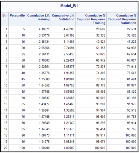
The lift for any percentile (bin) is the ratio of the observed response rate in the percentile to the overall observed response rate in the data set. The capture rate (% captured response) for any percentile shows the ratio of the number of observed responders within that percentile to the total number of observed responders in the data set. The cumulative lift and the lift are the same for the first percentile. However, the cumulative lift for the second percentile is the ratio of the observed response rate in the first two percentiles combined to the overall observed response rate. The observed response rate for the first two percentiles is calculated as the ratio of the total number of observed responders in the first two percentiles to the total number of records in the first two percentiles, and so on. The cumulative capture rate for the second percentile is the ratio of the number of observed responders in the first two percentiles to the total number of observed responders in the sample, and so on for the remaining percentiles.

For example, the last column for 40^th percentile shows that 76.543% of all responders are in the top 40% of the ranked data set. The ranking is done by the scores (predicted probability).

6.4.1.2 Model_B2

The middle section of the Display 6.54 shows the process flow for Model_B2. This model is built by using transformed variables. All interval variables are transformed by the Maximum Normal transformation. Display 6.59 shows the settings of the Transform Variables node for this model.

To include the original as well as transformed variables for consideration in the model, you can reset the Hide and Reject properties to No. However, in this example, I left these properties at the default value of Yes, so that Model_B2 is built solely on the transformed variables.

Display 6.59

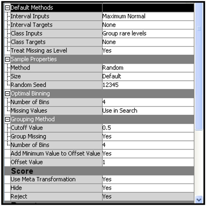
The value of the Interval Inputs property is set to Maximum Normal. This means that for each input $X$ $X$ , the transformations $\log (X)$ $\log (X)$ , $X^{1 / 4}$ $X^{1 / 4}$ , $s q r t (X)$ $s q r t (X)$ , $X^{2}$ $X^{2}$ , $X^{4}$ $X^{4}$ , and $e^{X}$ $e^{X}$ are evaluated. The transformation that yields sample quantiles that are closest to the theoretical quantiles of a normal distribution is selected. Suppose, by using one of these transformations, you get the transformed variable $Y$ $Y$ . This means that the 0.75_quantile for $Y$ $Y$ from the sample is that value of $Y$ $Y$ such that 75% of the observations are at or below that value of $Y$ $Y$ . The 0.75_quantile for a standard normal distribution is 0.6745 given by $P (Z \leq 0.6745) = 0.75$ $P (Z \leq 0.6745) = 0.75$ , where $Z$ $Z$ is a normal random variable with mean 0 and standard deviation 1. The 0.75_quantile for $Y$ $Y$ is compared with 0.6745; likewise, the other quantiles are compared with the corresponding quantiles of the standard normal distribution. To compare the sample quantiles with the quantiles of a standard normal distribution, you must first standardize the variables. Display 6.60 shows the standardization of the variable and the transformation that yielded maximum normality for each variable. In the code in this display, the variables Trans_SCALEVAR_100 and Trans_SCALEVAR_101 are the standardized variables.

Display 6.60

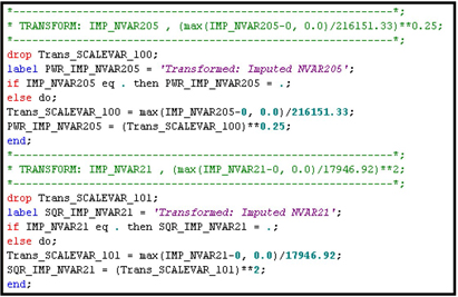
The variables are first scaled and then transformed, and the transformation that yielded quantiles closest to the theoretical normal quantiles is selected.

The Regression node properties settings are the same as those for Model_B1.

Display 6.61 shows the variables selected in the final model.

Display 6.61

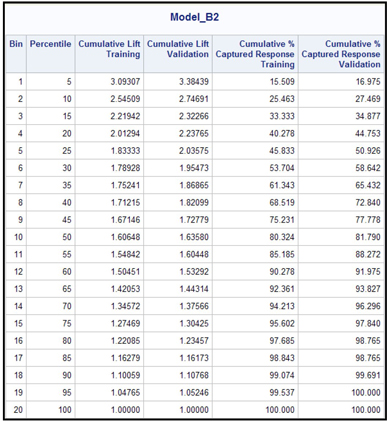
Display 6.62 shows the cumulative lift for the Training and Validation data sets.

Display 6.62

Display 6.62 shows that the model seems to make a better prediction for the Validation sample than it does for the Training data set. This does happen occasionally, and is no cause for alarm. It may be caused by the fact that the final model selection is based on the minimization of the validation error, which is calculated from the validation data set, since I set the Selection Criterion property to Validation Error.

When I allocated the data between the Training, Validation, and Test data sets, I used the default method, which is stratified partitioning with the target variable serving as the stratification variable. Partitioning done this way usually avoids the situations where the model performs better on the Validation data set than on the Training data set because of the differences in outcome concentrations.

The lift table corresponding to Display 6.62 and the cumulative capture rate are shown in Table 6.2.

Table 6.2

6.4.1.3 Model_B3

The bottom segment of Display 6.54 shows the process flow for Model_B3. In this case, the Decision Tree node is used for selecting the inputs. The inputs that give significant splits in growing the tree are selected. In addition, inputs selected for creating the surrogate rules are also saved and passed to the Regression node with their roles set to Input. The Decision Tree node also creates a categorical variable _NODE_. The categories of this variable identify the leaves of the tree. The value of the NODE_ variable, for a given record, indicates the leaf of the tree to which the record belongs. The Regression node uses _NODE_ as a class variable.

Display 6.63 shows the property settings of the Decision Tree node.

Display 6.63

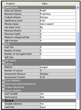
The Significance Level, Leaf Size, and the Maximum Depth properties control the growth of the tree, as discussed in as in Chapter 4. No pruning is done, since the Subtree Method property is set to Largest. Therefore, the Validation data set is not used in the tree development. As a result of the settings in the Output Variables and Score groups, the Decision Tree node creates a class variable _NODE_, which indicates the leaf node to which a record is assigned. The variable _NODE_ will be passed to the next node, the Regression node, as a categorical input, along with the other selected variables.

In the Model Selection group of the Regression node, the Selection Model property is set to Stepwise, and the Selection Criterion property to Validation Error. These are the same settings used earlier for Model_B1 and Model_B2.

The variables selected by the Regression Node are given in Display 6.64.

Display 6.64

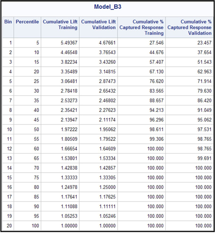
Display 6.65 shows the lift chart for the Training and Validation data sets. I saved the table behind these charts by clicking on the Table icon, clicking File→Save As, and then typing a data set name for saving the table. Table 6.3 is created from the saved SAS data set.

Display 6.65

Table 6.3

The three models are compared by the Model Comparison node.

Display 6.66 shows the lift charts for all three models together for the Training, Validation, and Test data sets.

Display 6.66

Click the Table icon located below the menu bar in the Results window to see the data behind the charts. SAS Enterprise Miner saves this data as a SAS data set. In this example, the data set is named &EM_LIB..MdlComp_EMRANK. Table 6.4 is created from this data set. It shows a comparison of lift charts and capture rates for the Test data set.

Table 6.4

This table can be used for selecting the model for scoring the prospect data for mailing. If the company has a budget that permits it to mail only the top five percentiles in Table 6.4, it should select Model_B3. The reason for this is that, from the row corresponding to 25^th percentile in Table 6.4, Model_B3 captures 70.28% of all responders, while Model_B1 captures 58.82% of the responders, and Model_B2 captures 51.70% of the responders. If the prospect data is scored using Model_B3, it is likely to get more responders per any given number of mailings at 25^th percentile.

You can also compare model performance e in terms of the ROC charts produced by the Model Comparison node. The ROC charts for the three models are shown in Display 6.67.

Display 6.67

An ROC curve is a plot of Sensitivity (True Positive Rate) versus 1-Specifity (False Positive Rate) at different cut-off values.

To draw an ROC curve of a model for a given data set, you have to classify each customer (record) in the data set based on a cutoff value and the predicted probability. If the predicted probability of response for a customer is equal to or greater than the cutoff value, then you classify the customer as responder (1) If not, you classify the customer as non-responder (0).

For given cutoff value, you may classify a true responder as responder or a true non-responder as responder. If a true responder is classified as responder, then it is called true positive, and the total number of true positives in the data set is denoted by TP. If a true non-responder classified as a responder, then it is called a false positive, and the total number of false positives is denoted by FP. If a true responder is classified as non-responder, it is called a false negative, and the number of false negatives is denoted by FN. If a true non-responder is classified as non-responder, then it is called a true negative, and the number of true negatives is denoted by TN.

The total number of true responders in a data set is TP + FN = P, and the total number of true non-responders is FP+T N = N.

For a given cutoff value, you can calculate Sensitivity and Specificity as follows:

\begin{array}{l} S e n s i t i v i t y = \frac{T P}{P} = T P R \\ S p e c i f i c i y = \frac{T N}{N} \\ 1- S p e c i f i c i y = \frac{N - T N}{N} = \frac{F P}{N} = F P R \end{array}

$\begin{array}{l} S e n s i t i v i t y = \frac{T P}{P} = T P R \\ S p e c i f i c i y = \frac{T N}{N} \\ 1- S p e c i f i c i y = \frac{N - T N}{N} = \frac{F P}{N} = F P R \end{array}$

An ROC curve is obtained by calculating sensitivity and specificity for different cutoff values and plotting them as shown in Display 6.67. See Chapter 5, Section 5.4.3 for a detailed description of how to draw ROC charts.

The size of the area below an ROC curve is an indicator of the accuracy of a model. From Display 6.67 it is apparent that the area below the ROC curve of Model_B3 is the largest for the Training, Validation, and Test data sets.

6.4.2 Regression for a Continuous Target

Now I turn to the second business application discussed earlier, which involves developing a model with a continuous target. As I did in the case of binary targets, in this example I build three versions of the model described above: Model_C1, Model_C2, and Model_C3. All three predict the increase in customers’ savings deposits in response to a rate increase, given a customer’s demographic and lifestyle characteristics, assets owned, and past banking transactions. My primary goal is to demonstrate the use of the Regression node when the target is continuous. In order to do this, I use simulated data of a price test conducted by a hypothetical bank, as explained at the beginning of Section 6.4.

The basic model is $\log (Δ D e p o s i t s_{i}_{t}) = β^{'} X_{i}$ $\log (Δ D e p o s i t s_{i}_{t}) = β^{'} X_{i}$ , where $Δ D e p o s i t s_{i t}$ $Δ D e p o s i t s_{i t}$ is the change in deposits in the $i^{t h}$ $i^{t h}$ account during the time interval $(t, t + Δ t)$ $(t, t + Δ t)$ . An increase in interest rate is offered at time $t$ $t$ . $β$ $β$ is the vector of coefficients to be estimated using the Regression node. $X_{i}$ $X_{i}$ is the vector of inputs for the $i^{t h}$ $i^{t h}$ account. This vector includes customers’ transactions prior to the rate change and other customer characteristics.

The target variable LDELBAL is $\log (Δ D e p o s i t s_{i}_{t})$ $\log (Δ D e p o s i t s_{i}_{t})$ for the models developed here. My objective is to find answers to this question: Of those who responded to the rate increase, which customers are likely to increase their savings the most? The change in deposits is positive by definition, but it is much skewed in the sample created. Hence, I made a log transformation of the dependent variable. When the model is created, you can score the prospects using either the estimated value of $\log (Δ D e p o s i t s_{i}_{t})$ $\log (Δ D e p o s i t s_{i}_{t})$ or $Δ D e p o s i t s_{i}_{t}$ $Δ D e p o s i t s_{i}_{t}$ .

Display 6.68 shows the process flow for the three models to be tested.

Display 6.68

The SAS data set containing the price test results is read by the Input Data Source node. From this data set, the Data Partition node creates the three data sets Part_Train, Part_Validate, and Part_Test with the roles Train, Validate, and Test, respectively. 40% of the records are randomly allocated for Training, 30% for Validation, and 30% for Test.

Display 6.69 shows the property settings for the Regression node. It is the same for all three models.

Display 6.69

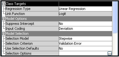
In addition to the above settings, the Entry Significance Level property is set to 0.1, and the Stay Significance Level property is set to 0.05.

6.4.2.1 Model_C1

The top section of Display 6.68 shows the process flow for Model_C1. In this model, the inputs are used without any transformations. The target is continuous; therefore, the coefficients of the regression are obtained by minimizing the error sums of squares.

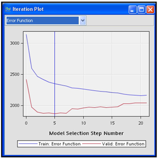
From the Iteration Plot shown in Display 6.70 it can be seen that the stepwise selection process took 21 steps to complete the effect selection. After the 21^th step, no additional inputs met the 0.1 significance level for entry into the model. The selected model is the one trained at Step 5 since it has the smallest validation error. Display 6.71 shows the selected model.

Display 6.70

Display 6.71

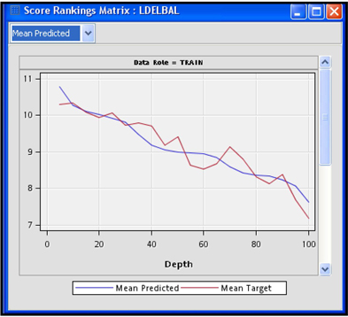
Display 6.72 shows the plot of the predicted mean and actual mean of the target variable by percentile.

Display 6.72

The Regression node appends the predicted and actual values of the target variable for each record in the Training, Validation, and Test data sets. These data sets are passed to the SAS Code node.

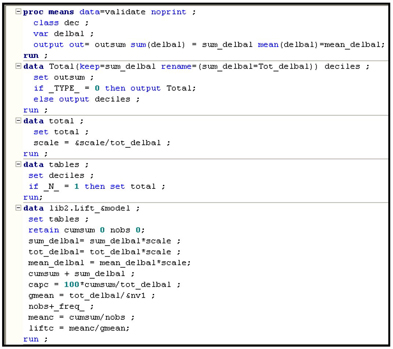
Table 6.5 is constructed from the Validation data set. When you run the Regression node, it calculates the predicted values of the target variable for each record in the Training, Validation, and Test data sets. The predicted value of the target is P_LDELBAL in this case. This new variable is added to the three data sets.

In the SAS Code node, I use the Validation data set’s predicted values in P_LDELBAL to create the decile, lift, and capture rates for the deciles. The program for these tasks is shown in Displays 6.73A, 6.73B, and 6.73C.

Table 6.5 includes special lift and capture rates that are suitable for continuous variables in general, and for banking applications in particular.

Table 6.5

The capture rate shown in the last column of Table 6.5 indicates that if the rate incentive generated an increase of $10 million in deposits, 9.3% of this increase would be coming from the accounts in the top percentile, 18.5% would be coming from the top two percentiles, and so on. Therefore, by targeting only the top 50%, the bank can get 76.3% of the increase in deposits.

By looking at the last row of the Cumulative Mean column, you can see that the average increase in deposits for the entire data set is $11,416. However, the average increase for the top demi-decile is $21,705 – almost double the overall mean. Hence, the lift for the top percentile is 1.90. The cumulative lift for the top two percentiles is 1.86, and so on.

Display 6.73A

Display 6.73B (continued from Display 6.73A)

Display 6.73C (continued from Display 6.73B)

6.4.2.2 Model_C2

The process flow for Model_C2 is given in Display 6.68. The Transform Variables node creates three data sets: Trans_Train, Trans_Validate, and Trans_Test. These data sets include the transformed variables. The interval inputs are transformed by the Maximum Normal method, which is described in Section 2.9.6 of Chapter 2. In addition, I set the Class Inputs property to Dummy indicators and Treat Missing as Level property to Yes in the Transformation node. In the Regression node, the effect selection is done by using the Stepwise method, and the Selection Criterion property is set to Validation Error.

Display 6.74 shows the Score Rankings in the Regression node’s Results window.

Display 6.74

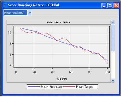
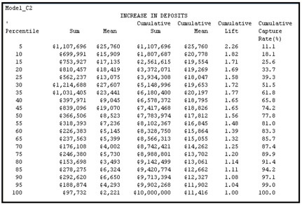
Table 6.6 shows the lift and capture rates of Model_C2.

Table 6.6

6.4.2.3 Model_C3

The process flow for Model_C3 is given in the lower region of Display 6.68. After the missing values were imputed, the data was passed to the Decision Tree node, which selected some important variables and created a class variable called _NODE_. This variable indicates the node to which a record belongs. The selected variables and special class variables were then passed to the Regression node with their roles set to Input. The Regression node made further selections from these variables, and the final equation consisted of only the _NODE_ variable. In the Decision Tree node, I set the Subtree Method property to Largest, and in the Score group, I set the Variable Selection property to Yes and the Leaf Role property to Input.

Display 6.75 shows the Score Rankings in the Regression node’s Results window.

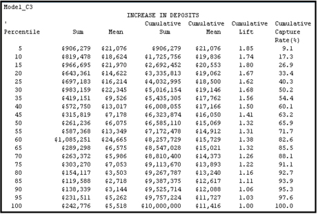
Display 6.75

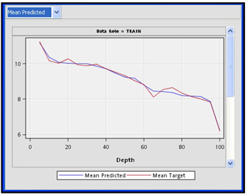
Table 6.7

A comparison of Model_C1, Model_C2, and Model_C3 is shown in Table 6.8.

Table 6.8

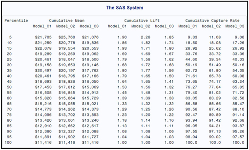
The cumulative capture rate at 50^th percentile is 77.84 for Model_C2, Therefore, by targeting the top 50% given by Model_C2, the bank can get 77.84% of the increase in deposits. The cumulative capture rates for Model_C1 and Model_C3 are smaller than for Model_C3 at the 50^th percentile.

6.5 Summary

• Four types of models are demonstrated using the Regression Node. These are models with binary, ordinal, nominal (unordered) and continuous targets.

• For each model, the underlying theory is explained with equations which are verified from the SAS code produced by the Regression Node.

• The Regression Type, Link Function, Selection Model, and Selection Options properties are demonstrated in detail.

• A number of examples are given to demonstrate alternative methods of model selection and model assessment by setting different values to the Selection Model and Selection Criterion properties. In each case, the produced output is analyzed.

• Various tables produced by the Regression Node and the Model Comparison Node are saved and other tables are produced from them.

• Two business applications are demonstrated - one requiring a model with binary target, and the other a model with continuous target.

1) The model with binary target is for identifying the current customers of a hypothetical bank who are most likely to respond to a monetarily rewarded invitation to sign up for Internet banking.

2) The model with continuous target is for identifying customers of a hypothetical bank who are likely to increase their savings deposits by the largest dollar amounts if the bank increases the interest paid to them by a preset number of basis points.

3) Three models are developed for each application and the best model is identified.

6.6 Appendix to Chapter 6

SAS code used to generate Table 6.1.

Display 6.76

Display 6.77

Display 6.78

Display 6.79

Display 6.80

6.6 Exercises

1. Create a data source using the dataset TestSelection.

a. Customize the metadata using the Advanced Metadata Advisor Options. Set the Class Levels Threshold property to 8.

b. Set the role of the variable RESP to Target.

c. Enter the following Decision Weights: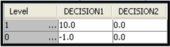

2. Add a Data Partition node to the process flow and allocate 40% of the records for Training, 30% for Validation and 30% for the Test data set.

3. Add a Regression node to the process flow and set the following properties:

a. Selection Model property to Forward

b. Selection Criterion to Schwarz Bayesian Criterion

c. Use Selection Defaults property to Yes

4. Run the Regression node.

5. Plot the Schwarz’s Bayesian Criterion at each step of the iteration.

6. Change the Selection Criterion to Akaike Information Criterion.

7. Repeat steps 4 and 5.

8. Compare the iteration plots and the selected models.

Notes

1. Despite the fact that Intercept 2 is not statistically significant, I show the calculations to illustrate the proportional odds model.

2. Ramon C. Littell, Rudolf J. Freund, and, Philip C. Spector. SAS System for Linear Models (Cary, NC: SAS Institute Inc., 1991), 21, 22, 156.

3. Littell, Freund, and Spector, SAS System for Linear Models.

4. For the computation of the score Chi-Square statistic, see “The LOGISTIC Procedure” in SAS/STAT® User’s Guide.

5. My explanations of the procedures described here are not written from the actual computational algorithms used inside SAS Enterprise Miner. I have no access to those. There may be some variance between my descriptions and the actual computations in some places. Nonetheless, these explanations should provide a clear view of how the various criteria of model selection are applied in general, and can most certainly be applied using SAS Enterprise Miner.

..................Content has been hidden....................

You can't read the all page of ebook, please click here login for view all page.

Table of Contents for Chapter 6: Regression Models

Create new playlist

Sign In

Sign Up

Chapter 6: Regression Models

6.1 Introduction