This chapter shows you how to build decision tree models to predict a categorical target and how to build regression tree models to predict a continuous target. Two examples are presented. The first example shows how to build a decision tree model to predict response to direct mail. In this example, the target variable is binary, taking on the values response and no response. The second example shows how to build a regression tree model to forecast a continuous (but interval-scaled) target often used in the auto insurance industry, namely loss frequency (described in Chapter 1). Loss frequency can also be modeled as a categorical target variable if it takes on only a few values but in this example it is treated as a continuous target.

4.2 An Overview of the Tree Methodology in SAS Enterprise Miner

4.2.1 Decision Trees

A decision tree represents a hierarchical segmentation of the data. The original segment is the entire data set, and it is called the root node of the tree. The original segment is first partitioned into two or more segments by applying a series of simple rules. Each rule assigns an observation to a segment based on the value of an input (explanatory variable) for that observation. In a similar fashion, each resulting segment is further partitioned into sub-segments (segments within a segment); each sub-segment is further partitioned into more sub-segments, and so on. This process continues until no more partitioning is possible. This process of segmenting is called recursive partitioning, and it results in a hierarchy of segments within segments. The hierarchy is called a tree, and each segment or sub-segment is called a node.

Sometimes the term parent node is used to refer to a segment that is partitioned into two or more sub-segments. The sub-segments are called child nodes. When a child node itself is partitioned further, it becomes a parent node.

Any segment or sub-segment that is further partitioned into more sub-segments can also be called an intermediate node. A node with all its successors forms a branch of the tree. The final segments that are not partitioned further are called terminal nodes or leaf nodes or leaves of the tree. Each leaf node is defined by a unique combination of ranges of the values of the input variables. The leaf nodes are disjoint subsets of the original data. There is no overlap between them, and each record in the data set belongs to one and only one leaf node. In this book, I sometimes refer to a leaf node as a group or segment.

4.2.2 Decision Tree Models

A decision tree model is composed of several parts:

• node definitions, or rules, to assign each record of a data set to a leaf node

• posterior probabilities of each leaf node

• the assignment of a target level to each leaf node

Node definitions are developed using the Training data set and are stated in terms of input ranges. Posterior probabilities are calculated for each node using the Training data set. The assignment of the target level to each node is also done during the training phase using the Training data set.

Posterior probabilities are observed proportions of target levels within each node in the training data set. Take the example of a binary target. A binary target has two levels, which can be represented by response and no response, or 1 and 0. The posterior probability of response in a node is the proportion of records with the target level equal to response, or 1, within that node. Similarly, the posterior probability of no response of a node is the proportion of records with the target level equal to no response, or 0, within that node. These posterior probabilities are determined during the training of the tree and they become part of the decision tree model. As mentioned above, they are calculated using the training data.

The assignment of a target level to an individual record, or to a node as a whole, is called a decision. The decisions are made in order to maximize profit, minimize cost, or minimize misclassification error. To illustrate a decision based on profit maximization, consider the example of a binary target. In order to maximize profits, you need a profit matrix. For illustrative purposes, I devised the profit matrix given in Table 4.1.

Table 4.1

	Decision1	Decision2
Actual target level/class
1	$10	0
0	-$1	0

In Table 4.1, Decision1 means assigning a record to the target level 1 (response), and Decision2 means assigning a record to target level 0 (non-response). This profit matrix indicates that if a true responder is correctly classified as a responder, then the profit earned is $10. If a true non-responder is classified as responder, a loss of $1 is incurred. If a true responder is classified as non-responder, then the profit is zero.¹ If a true non-responder is classified as a non-responder, then also the profit is zero.

Suppose $E_{1}$ $E_{1}$ represents the expected profit under Decision1, and $E_{2}$ $E_{2}$ represents the expected profit under Decision2. If $E_{1} > E_{2}$ $E_{1} > E_{2}$ then Decision1 is taken, and the record is assigned to the target level 1. If $E_{2} > E_{1}$ $E_{2} > E_{1}$ then Decision2 is taken, and the record is assigned to the target level 0. Given a profit matrix, $E_{1}$ $E_{1}$ and $E_{2}$ $E_{2}$ are based on the posterior probabilities of the node to which the record belongs. In general, each record is assigned the posterior probabilities of the node in which it resides. The expected profits ( $E_{1}$ $E_{1}$ and $E_{2}$ $E_{2}$ ) are calculated as $E_{1} = 10 * {\hat{P}}_{1} - 1 * {\hat{P}}_{0}$ $E_{1} = 10 * {\hat{P}}_{1} - 1 * {\hat{P}}_{0}$ and $E_{2} = 0 * {\hat{P}}_{1} + 0 * {\hat{P}}_{0}$ $E_{2} = 0 * {\hat{P}}_{1} + 0 * {\hat{P}}_{0}$ for each record, where ${\hat{P}}_{1}$ ${\hat{P}}_{1}$ and ${\hat{P}}_{0}$ ${\hat{P}}_{0}$ represent the posterior probabilities of response and no response for the record.

It follows from these profit equations that all the records in a node have the same posterior probabilities, and are therefore assigned to the same target level.

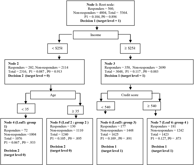
An example of a tree is shown in Figure 4.1. The tree shown in Figure 4.1 is handcrafted² in order to highlight the process of assigning target levels to the nodes.

Figure 4.1

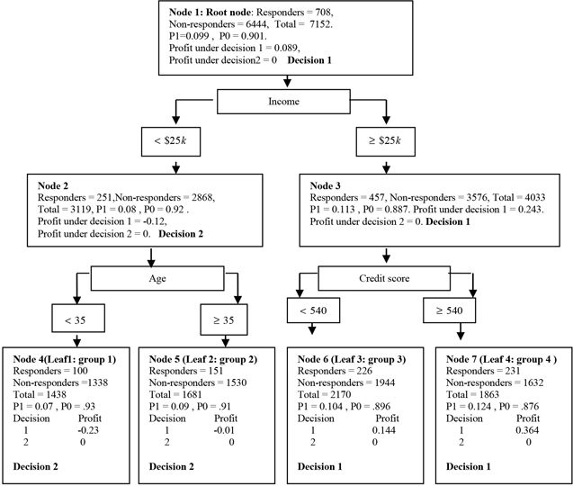
Figure 4.1 is an example of a tree for the target variable response. This variable has two levels: 1 for response and 0 for no response. Each node gives the information on the number of responders and non-responders, the proportion of responders (P1) and non-responders (P0), the decision regarding the assignment of a target level to the node, and the profit under each decision for that node.

Section 4.3.5 gives a step-by-step illustration of how SAS Enterprise Miner derives the information given in each node of the tree.

4.2.3 Decision Tree Models vs. Logistic Regression Models

A decision tree model is composed of a set of rules that can be applied to partition the data into disjoint groups. Unlike the logistic regression model, the tree model does not have any equations or coefficients. Instead, for each disjoint group or leaf node, it contains posterior probabilities which are themselves used as predicted probabilities. These posterior probabilities are developed during the training of the tree.

4.2.4 Applying the Decision Tree Model to Prospect Data

The SAS code generated by the Tree node can be applied to the prospect data set for purposes of prediction and classification. The code places each record in one of the predefined leaf nodes. The predicted probability of a target level (such as response) for each record is the posterior probability associated with the leaf node into which the record is placed. Since a target level is assigned to each leaf node, all records that fall into a leaf node are assigned the same target level. For example, the target level might be responder or non-responder.

4.2.5 Calculation of the Worth of a Tree

There are situations in which you must calculate the worth of a tree. The worth of a tree can be calculated using the Validation data set, Test data set, or any other data set where the target levels are known and the inputs necessary for defining the leaf nodes are available. Only leaf nodes are used for calculating the worth.

In SAS Enterprise Miner, the worth of a tree is calculated by using the validation data set to compare trees of different sizes in order to pick the tree with the optimum number of leaves. The worth of a tree can also be calculated using the test data in order to compare the performance of the decision tree model with other models. In both the cases, the method of calculating the worth of a tree is the same.

The following example calculates the worth of a tree using the Validation data set. The example uses a response model with a binary target. The binary target has two levels or classes: response (indicated by 1) and no response (indicated by 0). I use profit as a measure of worth, and show how the profits of the leaf nodes of a tree are calculated using the profit matrix introduced in Table 4.1. The calculation is a two-step procedure.

In Step 1, each record from the Validation data set is assigned to a leaf node based on rules or node definitions that are developed during the training phase. As noted above, all records that are placed in a particular leaf node are assigned the same posterior probabilities that were computed for that leaf node during the training phase using the training data set. Similarly, all records that fall into a particular leaf node are assigned the same target class/level (responder or non-responder) that was determined for that leaf node during training.

In Step 2, the profit is calculated for each leaf node of the tree based on the actual value of the target in each record of the validation data set.

If a leaf node is classified as a responder node (assigned the target level of 1), having $n_{1}$ $n_{1}$ records with the actual target level of 1 and $n_{0}$ $n_{0}$ records with the actual target level of 0, then the profit of that leaf node is $n_{1} * $ 10 + n_{0} * (- $ 1)$ $n_{1} * $ 10 + n_{0} * (- $ 1)$ . If, on the other hand, the leaf node is classified as a non-responder node, then the profit of that node is $n_{1} * $ 0 + n_{0} * $ 0$ $n_{1} * $ 0 + n_{0} * $ 0$ . Following this procedure, the profit of each leaf node of the tree is calculated and then summed to calculate the total profit of the tree. The average profit of the tree is the total profit divided by the total number of records in the tree.

You can also calculate the total profit and average profit of a decision tree model using the Test data set. This is normally done when you want to compare the performance of a decision tree model to other models.

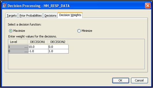
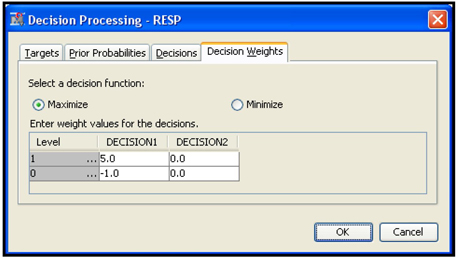
In SAS Enterprise Miner, you can enter the profit matrix when you create a data source, as shown in Chapter 2, Displays 2.14, 2.15, 2.16, and 2.17. You can also enter it by selecting the Input Data node and clicking located to the right of the Decisions property. Click the Decision Weights tab and enter the profit matrix, shown in Display 4.1.

Display 4.1

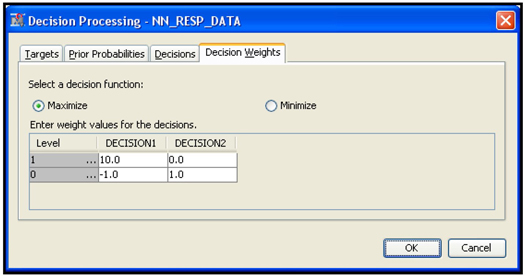
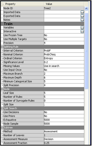
Display 4.1 also shows that I selected the decision function Maximize. The next step is to tell the Decision Tree node to use the profit matrix and the decision function I selected. I select the Decision Tree node. In the Subtree section in the Properties panel of the Decision Tree node (shown in Display 4.2), I set the Method property to Assessment and the Assessment Measure property to Decision.

Display 4.2

In SAS Enterprise Miner, profit is not the only criterion that can be used for calculating the worth of a tree. You can see the available criteria or measures by clicking in the Value column of the Assessment Measure property. The assessment measures are Decision, Average Square Error, Misclassification, and Lift.

Following is a brief description of each measure of model performance. For further details, see the SAS Enterprise Miner Help.

Decision

If you enter a profit matrix and select the decision function Maximize (as in Display 4.1), then SAS Enterprise Miner calculates average profit as a measure of the worth of a tree and selects a tree so as to maximize that value. If you select the decision function Minimize, then SAS Enterprise Miner minimizes cost in selecting a tree.

Average Squared Error

This is the average of the square of the difference between the predicted outcome and the actual outcome. This measure is more appropriate when the target is continuous.

Misclassification

Using the example of a response model, if the model classifies a responder as a non-responder or non-responder as responder, then the result is a misclassification. The misclassification rate is inversely related to the worth of a tree. Selecting this option instructs SAS Enterprise Miner to select a tree so as to minimize the number of misclassifications.

Lift

In the case of a response model, which has a binary target, the lift is calculated as the ratio of the actual response rate of the top n% of the ranked observations in the validation data set to the overall response rate of the validation data set. The ranking is done by the predicted probability of response for each record in the validation data set.

The percentage of ranked data (n%) to be used as the basis for the lift calculation is specified by setting the Assessment Fraction property of the Decision Tree node. The default value is 0.25 (25%).

4.2.6 Roles of the Training and Validation Data in the Development of a Decision Tree

To develop a tree model, you need two data sets. The first is for training the model, and the second is for pruning or fine-tuning the model. A third data set is optionally needed for an independent assessment of the model. These three data sets are referred to in SAS Enterprise Miner as Training, Validation, and Test, respectively. You can decide what percentage of the model data set is to be allocated to each of these three purposes. While there are no uniform rules for allocation, you can follow certain rules of thumb. If the data available for modeling is large, you can allocate it equally between the three data sets. If that is not the case, use something like 40%, 30%, and 30%, or 50%, 25%, and 25%. This partitioning is done by specifying the values for the Training, Validation, and Test properties of the Data Partition node. Reserving more data for the training generally results in more stable parameter estimates.

4.2.6.1 Training Data

The Training data set is used to perform three main tasks:

• developing rules to assign records to nodes (node definitions)

• calculating the posterior probabilities (the proportion of cases or records in each level of the target) for each node

• assigning each node to a target level (decision)

4.2.6.2 Validation Data

The Validation data set is used to prune the tree, i.e., select the right-sized tree or optimal tree. The initial tree is usually large. This is called the maximal tree. Some call it the whole tree. In this book, I use these two terms interchangeably.

By removing certain branches of the maximal tree, I can create smaller trees. By removing a different branch, I get a different tree. The smallest of these trees has only one leaf, called the root node, and the largest is the initial maximal tree, which can have many leaves. Thus removing different branches produces a number of possible sub-trees. You must select one of them. Validation data is used for selecting a sub-tree.

As explained in Section 4.2.5, the worth of each tree of a different size is calculated using the Validation data set, and one of the measures of worth is profit. Since profit is calculated using records of the Validation data set, profit is referred to as the validation profit in SAS Enterprise Miner.

Validation profit is used to select the optimal (right-sized) tree. The size of a tree is defined as the number of leaves in the tree. An optimal tree is defined as that tree that yields higher profit than any smaller tree (tree with fewer leaves) and equal or higher profit than any larger tree.

Since it is easy to travel from node to node and construct trees that end up with, say, ten leaves, there may be more than one tree of a given size within the maximal (or whole) tree. SAS Enterprise Miner searches through all the possible trees to find the one with the highest validation profit. Details of this search process are discussed in section 4.3.

4.2.6.3 Test Data

The Test data set is used for an independent assessment of the final model, particularly when you want to compare the performance of a decision tree model to the performance of other models.

4.2.7 Regression Tree

When the target is continuous, the tree is called a regression tree. The regression tree model consists of the rules (node definitions) for partitioning the data set into leaf nodes and also the mean of the target for each leaf node.

4.3 Development of the Tree in SAS Enterprise Miner

Construction of a decision tree or regression tree involves two major steps. The first step is growing a large tree. As mentioned before, you can then create many smaller trees, called sub-trees, of different sizes by removing one or more branches of the large tree. The second step is selecting the optimal sub-tree. SAS Enterprise Miner offers a number of choices for performing these steps. The following sections show how to use these methods by setting various properties.

4.3.1 Growing an Initial Tree

As described in Section 4.2.1, growing a tree involves successively partitioning the data set into segments using the method of recursive partitioning. Here I discuss how the inputs are selected at each step of the sequence of recursive partitioning. I focus on two-way, or binary, splits of the inputs, although SAS Enterprise Miner can also perform three-way and multi-way splits. In addition, the discussion assumes that the target is binary.

4.3.1.1 How a Node is Split Using a Binary Split Search

In a binary split, two branches emerge from each node. When an input such as household income is used to partition the records into two groups, a splitting value such as the household income value of $10,000 may be chosen. The records with income less than the splitting value are sent to the left branch, and records with income greater than or equal to the splitting value are sent to the right branch. In a multi-way split, more than two branches may emerge from any node. For example, the income variable could be divided into ranges such as $0–$10,000, $10,001–$20,000, $20,001– $30,000, etc. As mentioned earlier, for the purposes of simplicity and clarity, I confine my discussion to two-way splits across an input.

In order to split any segment or sub-segment of the data set at a node, SAS Enterprise Miner calculates the worth of all candidate splitting values for each of the inputs and selects the split with the highest worth, which involves finding the best splitting value for each of the available inputs and then comparing all of the inputs to see which one’s split is best. You can select the method of calculating the worth of the split. These methods are discussed in the following sections.

The process of selecting the best split consists of two steps. In the first step, the best splitting value for each input is determined. In the second step, the best input among all inputs is selected by comparing the worth of the best split of each variable with the best splits of the others, and selecting the input whose best split yields the highest worth. The node is split at the best splitting value on the best input. The following example illustrates this process.

Suppose there are 100 inputs, represented by $X_{1}, X_{2}, ..., X_{100}$ $X_{1}, X_{2}, ..., X_{100}$ . The tree algorithm starts with input $X_{1}$ $X_{1}$ and examines all candidate splits of the form $X_{1} < C,$ $X_{1} < C,$ where $C$ $C$ is a splitting value somewhere between the minimum and maximum value of $X_{1}$ $X_{1}$ . All records that have $X_{1} < C$ $X_{1} < C$ go to the left child node and all records that have $X_{1} \geq C$ $X_{1} \geq C$ go to the right child node. The algorithm goes through all candidate splitting values on the same input and selects the best splitting value. Let the best splitting value on input $X_{1}$ $X_{1}$ be $C_{1}$ $C_{1}$ . The algorithm repeats the same process on the next input $X_{2}$ $X_{2}$ . This process is repeated on inputs $X_{2}, X_{3}, X_{4}, ..., X_{100}$ $X_{2}, X_{3}, X_{4}, ..., X_{100}$ and the corresponding best splitting values $C_{2}, C_{3}, C_{4}, ..., C_{100}$ $C_{2}, C_{3}, C_{4}, ..., C_{100}$ are found. Having found the best splitting value for each input, the algorithm then compares these splits to find the input whose best splitting value gives a better split of the data than the best splitting value of any other input. Suppose $C_{10}$ $C_{10}$ is the best splitting value for input $X_{10}$ $X_{10}$ and suppose $X_{10}$ $X_{10}$ is chosen as the best input upon which to base a split of the node. Consequently, the node is partitioned using the input $X_{10}$ $X_{10}$ . All records with $X_{10}$ $X_{10}$ less than $C_{10}$ $C_{10}$ are sent to the left child node and all records with $X_{10}$ $X_{10}$ $\geq$ $\geq$ $C_{10}$ $C_{10}$ are sent to the right child node. This process is repeated for each node. A different input may be chosen at a different node. How are the splits compared to determine the best splits? To answer this, it is necessary to examine how we measure the worth of each split.

4.3.1.2 Measuring the Worth of a Split (Splitting Criterion Property of the Decision Tree Node in SAS Enterprise Miner)

The splitting method used for partitioning the data is determined by the value of the Criterion property in the Splitting Rule section of the Properties panel. If your target variable is nominal, then click in the column to the right of the Nominal Criterion property to see the various methods of splitting, as shown in Display 4.3.

Display 4.3

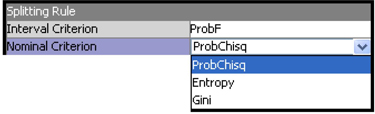
A nominal variable is a variable that takes on values such as Response and No Response. The values that a nominal variable takes on are sometimes referred to as levels or categories. In this example, the target variable, Resp, takes on only two values—response and no response. A nominal variable can take on more than two values. For example, a nominal variable Color can take the values such as Red, Blue, Green, etc. The important feature of a nominal variable is that the values that it takes on cannot be ranked according to any measurement scale. That is, Response is not higher or lower than No response; Blue is not higher or lower than Green. In general, we can say that a nominal variable is a categorical variable having unordered levels or categories. When a nominal variable has only two levels, it can be referred to as a binary variable. In our example, since we are considering a target variable that takes the values Response and No response, which do not represent any order, our target variable is a nominal target. Since it takes only two values, we can call it a binary variable. We can also call it a categorical variable having unordered scales since the levels or categories or the values that it takes on are not ordered.

If your target is a categorical variable with ordered scales, then it is called an ordinal variable. An example of an ordinal variable is Risk, which can take on values such as High, Medium, and Low. Since High represents higher risk than Medium and Medium represents higher risk than Low, Risk is an ordinal variable.

If your target variable is ordinal, then click in the column to the right of the Ordinal Criterion property to see the methods of splitting that apply to the ordinal variable situation. The methods are Entropy and Gini.

A variable such as our Savings Account Balances variable is called an interval scaled variable.

If your target variable is an interval scaled variable, then click in the column to the right of the Interval Criterion property to see the methods of splitting that are appropriate for this situation, which are Variance and ProbF.

When the target variable is binary or categorical with more than two levels, there are two approaches for measuring the worth of a split:

• the degree of separation achieved by the split. In SAS Enterprise Miner, this is measured by the p-value of the Pearson Chi-Square test.

• the impurity reduction achieved by the split. In SAS Enterprise Miner, this is measured either by Entropy reduction or by Gini reduction.

When the target is continuous, SAS Enterprise Miner measures the worth of a split by an F-test, which tests for the degree of separation of the child nodes. If you set the Interval Criterion to Variance, Variance Reduction is used to measure the worth of a split. This chapter looks at these measures case by case.

4.3.1.2A Measuring the Worth of a Split When the Target is Binary

4.3.1.2A.1 Degree of Separation

Any two-way split partitions a parent node into two child nodes. Logworth is a measure of how different these child nodes are from each other and from the parent node, in terms of the composition of the classes. The greater the difference between the two child nodes, the greater the degree of separation achieved by the split, and the better the split is considered to be.

To see how logworth is calculated at each splitting value, consider this example. Let the target be response, and let household income be an input (explanatory variable). Let each row of the data set represent a record (or observation) from the data set. Table 4.2 shows a partial view of the data set, showing only selected records from the data set and only two columns. The records are in increasing order of income, to help discuss the notion of splitting the records on the basis of income.

Table 4.2

Observation (record)	Response	Household income
1	1	$8,000
2	0	$10,000
...	...	...
100	1	$12,000
...	...	...
1200	0	$14,000
...	...	...
...	...	...
10,000	1	$150,000

The data shown in Table 4.2 can be split at different values of household income. At each splitting value, a 2x2 contingency table can be constructed, as shown in Table 4.3. Table 4.3 shows an example of one split. The columns represent the two child nodes that result from the split, and rows represent the levels of the target.

Table 4.3

	$Income < $ 10, 000$ $Income < $ 10, 000$	$Income \geq $ 10, 000$ $Income \geq $ 10, 000$	Total
Responders	$n_{11}$ $n_{11}$	$n_{12}$ $n_{12}$	$n_{1 •}$ $n_{1 •}$
Non-responders	$n_{01}$ $n_{01}$	$n_{02}$ $n_{02}$	$n_{0 •}$ $n_{0 •}$
Total	$n_{• 1}$ $n_{• 1}$	$n_{• 2}$ $n_{• 2}$	$n$ $n$

To assess the degree of separation achieved by a split, you must calculate the value of the Chi-Square ( $χ^{2}$ $χ^{2}$ ) statistic and test the null hypothesis that the proportion of responders among those with income less than $10,000 is not different from those with income greater than or equal to $10,000. This can be written as:

H_{0} : P_{1} = P_{2} = P

$H_{0} : P_{1} = P_{2} = P$

Let {\hat{P}}_{1} = \frac{n_{11}}{n_{• 1}}, {\hat{P}}_{2} = \frac{n_{12}}{n_{• 2}} and \hat{P} = \frac{n_{1 •}}{n}

$Let {\hat{P}}_{1} = \frac{n_{11}}{n_{• 1}}, {\hat{P}}_{2} = \frac{n_{12}}{n_{• 2}} and \hat{P} = \frac{n_{1 •}}{n}$

Under the null hypothesis, the expected values are:

	$Income < $ 10, 000$ $Income < $ 10, 000$	$Income \geq $ 10, 000$ $Income \geq $ 10, 000$
Responders	$E_{11} = \hat{P} \times n_{• 1}$ $E_{11} = \hat{P} \times n_{• 1}$	$E_{12} = \hat{P} \times n_{• 2}$ $E_{12} = \hat{P} \times n_{• 2}$
Non-responders	$E_{01} = (1 - \hat{P}) \times n_{• 1}$ $E_{01} = (1 - \hat{P}) \times n_{• 1}$	$E_{02} = (1 - \hat{P}) \times n_{• 2}$ $E_{02} = (1 - \hat{P}) \times n_{• 2}$

The Chi-Square statistic is calculated as follows:

χ^{2} = \sum_{i = 0}^{1} \sum_{j = 1}^{2} \frac{{(n_{i j} - E_{i j})}^{2}}{E_{i j}}

$χ^{2} = \sum_{i = 0}^{1} \sum_{j = 1}^{2} \frac{{(n_{i j} - E_{i j})}^{2}}{E_{i j}}$

The p-value of $χ^{2}$ $χ^{2}$ is found by solving the equation:

P( $χ^{2}$ $χ^{2}$ > calculated $χ^{2}$ $χ^{2}$ | null hypothesis is true)= p-value. And the logworth is simply calculated as $L o g w o r t h = - l o g_{10} (p - v a l u e)$ $L o g w o r t h = - l o g_{10} (p - v a l u e)$ .

The larger the logworth (and therefore the smaller the $p - value$ $p - value$ ), the better the split.

Let the logworth calculated from the first split be $L W_{1}$ $L W_{1}$ . Another split is made at the next level of income (for example $12,000), a contingency table is made, and the logworth is calculated in the same way. I call this $L W_{2}$ $L W_{2}$ . If there are 100 distinct values for income in the data set, 99 contingency tables can be created, and the logworth computed for each. The calculated values of the logworth are $L W_{1}$ $L W_{1}$ , $L W_{2}$ $L W_{2}$ ,..., $L W_{99}$ $L W_{99}$ . The split that generates the highest logworth is selected. Suppose the best splitting value for income is $15,000, with a logworth of 20.5. Now consider the next variable, Age. If there are 67 distinct values of Age in the data set, 66 splits are considered; the split with the maximum logworth is selected for Age. Suppose the best splitting value for Age is 35, with a logworth of 10.2. If age and income are the only inputs in the data set, then income is selected to split the node because it has the best logworth value. In other words, the best split on income ($15,000) has a higher logworth (20.5) than the best split on Age (35) with a logworth of 10.2. Hence the data set would be split at $15,000 of income. This split can be called the best of the best.

If there were 200 inputs in the data set, the process of finding the best split is performed 200 times (once for each input), and repeated again at each node that is further split. Each input is examined, the best split found, and the one with the highest logworth chosen as the best of the best.

To use the Chi-Square method of choosing a split, set the Nominal Criterion property in the Splitting Rule section of the Decision Tree node to ProbChisq.

4.3.1.2A.2 Impurity Reduction as a Measure of Goodness of a Split

In SAS Enterprise Miner, you can choose maximizing impurity reduction as an alternative to maximizing the degree of separation for selecting the splits on a given input, and for selecting the best input. The impurity of a node is the degree of heterogeneity with respect to the composition of the levels of the target variable. If node $v$ $v$ is split into child nodes $a$ $a$ and $b,$ $b,$ and if $ω_{a}$ $ω_{a}$ and $ω_{b}$ $ω_{b}$ are the proportions of records in nodes $a$ $a$ and $b,$ $b,$ then the decrease in impurity is $i (v) - ω_{a} i (a) - ω_{b} i (b),$ $i (v) - ω_{a} i (a) - ω_{b} i (b),$ where $i (v)$ $i (v)$ is the impurity index of node $v,$ $v,$ and $i (a)$ $i (a)$ and $i (b)$ $i (b)$ are the impurity indexes of the child nodes $a$ $a$ and $b$ $b$ , respectively. In SAS Enterprise Miner there are two measures of impurity, one measure called the Gini Impurity Index, and the other called Entropy.

To split the node $v$ $v$ into child nodes $a$ $a$ and $b$ $b$ based on the splitting value of an input $X_{1}$ $X_{1}$ , the Tree algorithm examines all candidate splits of the form $X_{1} < C_{j}$ $X_{1} < C_{j}$ and $X_{1} \geq C_{j}$ $X_{1} \geq C_{j}$ , where $C_{j}$ $C_{j}$ is a real number between the minimum and maximum values of $X_{1}$ $X_{1}$ . Those records that have $X_{1} < C_{j}$ $X_{1} < C_{j}$ go to the left child node and those with $X_{1} \geq C_{j}$ $X_{1} \geq C_{j}$ go to the right. Suppose there are 100 candidate splitting values on the input $X_{1}$ $X_{1}$ . The candidate splitting values are $C_{j}, j = 1, 2, ....100$ $C_{j}, j = 1, 2, ....100$ . The algorithm compares impurity reduction on these 100 splits and selects the one that achieves the greatest impurity reduction as the best split.

4.3.1.2A.2.1 Gini Impurity Index

If $p_{1}$ $p_{1}$ is the proportion of responders in a node, and $p_{0}$ $p_{0}$ is the proportion of non-responders, the Gini Impurity Index of that node is defined as $i (p) =$ $i (p) =$ $1 - p_{1}^{2} - p_{0}^{2}$ $1 - p_{1}^{2} - p_{0}^{2}$ . If two records are chosen at random (with replacement) from a node, the probability that both are responders is $p_{1}^{2}$ $p_{1}^{2}$ , while the probability that both are non-responders is $p_{0}^{2}$ $p_{0}^{2}$ , and the probability that they are either both responders or both non-responders is $p_{1}^{2} + p_{0}^{2}$ $p_{1}^{2} + p_{0}^{2}$ . Hence $1 - p_{1}^{2} - p_{0}^{2}$ $1 - p_{1}^{2} - p_{0}^{2}$ can be interpreted as the probability that any two elements chosen at random (with replacement) are different. For binary targets, the Gini Index simplifies to $2 p_{1} (1 - p_{1}) .$ $2 p_{1} (1 - p_{1}) .$ A pure node has a Gini Index of zero. It has a maximum value of $1 / 2$ $1 / 2$ when both classes are equally represented. To use this criterion when your target variable is an unordered categorical variable, set the Nominal Criterion property in the Splitting Rule section to Gini. If your target variable is ordinal (ordered categorical), set the Ordinal Criterion property to Gini.

4.3.1.2A.2.2 Entropy

Entropy is another measure of the impurity of a node. It is defined as $i (p) =$ $i (p) =$ $- \sum_{i = 0}^{1} p_{i} \log_{2} (p_{i})$ $- \sum_{i = 0}^{1} p_{i} \log_{2} (p_{i})$ for binary targets. A node that has larger entropy than another is more heterogeneous and therefore less pure.

The rarity of an event is measured as $- \log_{2} (p_{i}) .$ $- \log_{2} (p_{i}) .$ If an event is rare, it means the probability of its occurrence is low. Consider the event Response. Suppose the probability of response in a node is 0.005. Then the rarity of response is $- \log_{2} (0.005) = 7.644.$ $- \log_{2} (0.005) = 7.644.$ This is a rare event. The probability of non-response is conversely 0.995, hence the rarity of non-response is $- \log_{2} (0.995) = 0.0072.$ $- \log_{2} (0.995) = 0.0072.$ A node that has a response rate of 0.005 is less impure than the node that has equal proportions of responders and non-responders. Thus $- \log_{2} (p_{i})$ $- \log_{2} (p_{i})$ is high when the rarity is high and low when the rarity of the event is low. The entropy of this node is as follows:

i (p) = - [0.005 * \log_{2} (0.005) + 0.995 * \log_{2} (0.995)] = 0.0454.

$i (p) = - [0.005 * \log_{2} (0.005) + 0.995 * \log_{2} (0.995)] = 0.0454.$

Consider another node in which the probability of response = probability of non-response = 0.5. The entropy of this node is $i (p) = - [0.5 * \log_{2} (0.5) + 0.5 * \log_{2} (0.5)] = 1.$ $i (p) = - [0.5 * \log_{2} (0.5) + 0.5 * \log_{2} (0.5)] = 1.$ The node that is predominantly non-responders (with a proportion of 0.995) has an entropy value of 0.0454. A node with an equal distribution of responders and non-responders has entropy equal to 1. A node that has all responders or all non-responders has an entropy equal to zero. Thus, entropy ranges between 0 to 1, with 0 indicating maximum purity and 1 indicating maximum impurity.

To use the Entropy measure when your target variable is an unordered categorical variable, go to the Splitting Rule section, and set the Nominal Criterion property to Entropy. If your target variable is ordinal (ordered categorical), rather than nominal, set the Ordinal Criterion property to Entropy.

4.3.1.3 Measuring the Worth of a Split When the Target is Categorical with More than Two Categories

If the target is categorical with more than two categories (levels), the procedures are the same. The Chi-Square statistics are calculated from $r$ $r$ x $b$ $b$ contingency tables, where $b$ $b$ is the number of child nodes being created on the basis of a certain input, and $r$ $r$ is the number of target levels (categories). The p-values are calculated from the Chi-Square distribution with degrees of freedom equal to $(r - 1) (b - 1) .$ $(r - 1) (b - 1) .$ The Gini Index and Entropy measures of impurity can also be applied in this case. They are simply extended for more than two levels (categories) of the target variable.

4.3.1.4 Measuring the Worth of a Split When the Target is Continuous

If the target is continuous, an F-test is used to measure the degree of separation achieved by a split. Suppose the target is loss frequency and the input is income having 100 distinct values. There are 99 possible two-way splits on income. At each split value, two groups are formed. One group has income level below the split value, and the other group has income greater than or equal to the split value. Consider a parent node with $n$ $n$ records and a split value of $10,000. All records with income less than $10,000 are sent to the left node and those with income greater than or equal to $10,000 are sent to the right node, as shown in Figure 4.2. The mean of the target is calculated for each node.

Figure 4.2

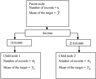
In order to calculate the worth of this split, a one-way ANOVA is first performed, and the logworth is then calculated from the F-test.

The Sum of Squares between the groups (child nodes) is given by:

\begin{array}{l} S S_{b e t w e e n} = \sum_{i = 1}^{2} n_{i} {({\bar{y}}_{i .} - {\bar{y}}_{..})}^{2}, where {\bar{y}}_{i .} is the mean of the target in the i^{t h} child node, and \\ {\bar{y}}_{..} is the mean of the target in the parent node . \end{array}

$\begin{array}{l} S S_{b e t w e e n} = \sum_{i = 1}^{2} n_{i} {({\bar{y}}_{i .} - {\bar{y}}_{..})}^{2}, where {\bar{y}}_{i .} is the mean of the target in the i^{t h} child node, and \\ {\bar{y}}_{..} is the mean of the target in the parent node . \end{array}$

The Sum of Squares within the groups (child nodes) is given by:

\begin{array}{l} S S_{w i t h i n} = \sum_{i = 1}^{2} \sum_{j = 1}^{n_{i}} {(y_{i j} - {\bar{y}}_{i .})}^{2}, where y_{i j} is the value of the target variable for \\ the j^{t h} record in the i^{t h} child node . \end{array}

$\begin{array}{l} S S_{w i t h i n} = \sum_{i = 1}^{2} \sum_{j = 1}^{n_{i}} {(y_{i j} - {\bar{y}}_{i .})}^{2}, where y_{i j} is the value of the target variable for \\ the j^{t h} record in the i^{t h} child node . \end{array}$

The Total Sum of Squares is given by

\begin{array}{l} S S_{t o t a l} = \sum_{i = 1}^{2} \sum_{j = 1}^{n_{i}} {(y_{i j} - {\bar{y}}_{..})}^{2}, and the F-statistic is computed as \\ F= (\frac{{SS}_{between} / (2 - 1)}{{SS}_{within} / (n - 2)}) . This statistic has an F-distribution with 1 and n - 2 degress \\ of freedom under the null hypohesis . \end{array}

$\begin{array}{l} S S_{t o t a l} = \sum_{i = 1}^{2} \sum_{j = 1}^{n_{i}} {(y_{i j} - {\bar{y}}_{..})}^{2}, and the F-statistic is computed as \\ F= (\frac{{SS}_{between} / (2 - 1)}{{SS}_{within} / (n - 2)}) . This statistic has an F-distribution with 1 and n - 2 degress \\ of freedom under the null hypohesis . \end{array}$

The null hypothesis says that there is no difference in the target mean between the child nodes.

The p-value is given by $P (F > c a l c u l a t e d F | null hypothesis is true) = p - value .$ $P (F > c a l c u l a t e d F | null hypothesis is true) = p - value .$

As before, the logworth is calculated from the p-value of the F-test as $- \log_{10} (p - value)$ $- \log_{10} (p - value)$ . The larger the logworth (and therefore the smaller the p-value), the better the split.

One-way analysis is performed at each splitting value on a given input such as income, the logworth of each split is calculated, and the split with the highest logworth is selected for the input. (If income is split into more than two groups, then one-way analysis is done with more than two groups.) As with the Chi-Square method and all the other methods, the same analysis is applied to each input, and the best split for each input is found. From the best splits of each input, the best input (the one with the highest logworth) is found, and that is the best of the best, that is, the best split on the best input.

To use the F-test shown earlier in this section, set the Interval Criterion property in the Splitting Rule section to ProbF, which is the default value for interval targets.

4.3.1.5 Impurity Reduction When the Target is Continuous

When the target is continuous, the sample variance can be used as a measure of impurity.

The impurity of the $t^{t h}$ $t^{t h}$ node is $i (t) = \frac{1}{n_{t}} {\sum_{j = 1}^{n_{t}} (y_{j t} - {\bar{y}}_{t})}^{2}$ $i (t) = \frac{1}{n_{t}} {\sum_{j = 1}^{n_{t}} (y_{j t} - {\bar{y}}_{t})}^{2}$ , where

$\begin{array}{l} i (t) = impurity of the t^{t h} node . \\ n_{t} = number observations in the t^{t h} node . \\ y_{j t} = value of the target variable in the j^{t h} observation in the t^{t h} node . \\ {\bar{y}}_{t} = mean of the target variable in the t^{t h} node . \end{array}$ $\begin{array}{l} i (t) = impurity of the t^{t h} node . \\ n_{t} = number observations in the t^{t h} node . \\ y_{j t} = value of the target variable in the j^{t h} observation in the t^{t h} node . \\ {\bar{y}}_{t} = mean of the target variable in the t^{t h} node . \end{array}$

The impurity of the root node (0) is $i (0) = \frac{1}{n_{0}} {\sum_{j = 1}^{n_{0}} (y_{j 0} - {\bar{y}}_{0})}^{2} .$ $i (0) = \frac{1}{n_{0}} {\sum_{j = 1}^{n_{0}} (y_{j 0} - {\bar{y}}_{0})}^{2} .$ If the root node is split into two child nodes 1 and 2, then the impurity reduction due the split is calculated as $Δ i = i (0) - {\frac{n_{1}}{n_{0}} i (1) + \frac{n_{2}}{n_{0}} i (2)}$ $Δ i = i (0) - {\frac{n_{1}}{n_{0}} i (1) + \frac{n_{2}}{n_{0}} i (2)}$ where $n_{0}$ $n_{0}$ is the number of observations in the root node, $n_{1}$ $n_{1}$ is the number of observations in the first child node and $n_{2}$ $n_{2}$ is the number of observations in the second child node. Impurity reduction can be used to measure the worth of a split. To use impurity reduction when the target is continuous, set the Interval Criterion in the Splitting Rule section to Variance.

4.3.2 P-value Adjustment Options

Using the default settings, SAS Enterprise Miner uses adjusted p-values in comparing splits on the same input and splits on different inputs. Two types of adjustments are made to $p - values$ $p - values$ : Bonferroni adjustment and Depth adjustment.

4.3.2.1 Bonferroni Adjustment Property

When you are comparing the splits from different inputs, p-values are adjusted to take into account the fact that not all inputs have the same number of levels. In general, some inputs are binary, some are ordinal, some are nominal, and others are interval-scaled. For example, a variable such as Mail Order Buyer takes on the value of 1 or 0, 1 being mail order buyer and 0 being not a mail order buyer. I will call this the Mail Order Buyer variable. For this variable, only one split is evaluated, only one contingency table is considered, and only one test is performed. An input like “number of delinquencies in the past 12 months” can take any value from 0 to 10 or higher. I will call this the Delinquency variable. This is an ordinal variable. Suppose it takes values from 0 to 10. SAS Enterprise Miner compares the split values 0.5, 1.5, 2.5,..., 9.5. Ten contingency tables are constructed, and ten Chi-Square values are calculated. In other words, ten tests are performed on this input for selecting the best split.

Suppose the $i^{t h}$ $i^{t h}$ split on the Delinquency variable has a $p - v a l u e = α_{i}$ $p - v a l u e = α_{i}$ , which means that P( $χ^{2}$ $χ^{2}$ $\geq$ $\geq$ calculated $χ_{i}^{2}$ $χ_{i}^{2}$ | null hypothesis is true)= $α_{i}$ $α_{i}$ . In other words, the probability of finding a Chi-Square greater than or equal to the calculated $χ_{i}^{2}$ $χ_{i}^{2}$ at random is $α_{i}$ $α_{i}$ under the null hypothesis. The probability that, out of the ten Chi-Square tests on the delinquency variable, at least one of the tests yields a false positive decision (where we reject the null hypothesis when it is actually true) is $1 - \prod_{i = 1}^{10} (1 - α_{i})$ $1 - \prod_{i = 1}^{10} (1 - α_{i})$ . This family-wise error rate is much larger than the individual error rate of $α_{i}$ $α_{i}$ . For example, if the individual error rate ( $α_{i}$ $α_{i}$ ) on each test =0.05, then the family-wise error rate is $1 - {0.95}^{10} =$ $1 - {0.95}^{10} =$ 0.401. This means that when you have multiple $χ_{i}^{2}$ $χ_{i}^{2}$ comparisons (one for each possible split), the p-values underestimate the risk of rejecting the null hypothesis when it is true. Clearly the more possible splits a variable has, the less accurate the p-values will be. Therefore, when comparing the best split on the Delinquency variable with the best split on the Mail Order Buyer variable, the logworths need to be adjusted for the number of splits, or tests, on each variable. In the case of the Mail Order Buyer variable, there is only one test, and hence no adjustment is necessary. But in the case of the Delinquency Variable, the best split is chosen from a set of ten splits. Therefore, $\log_{10} (10)$ $\log_{10} (10)$ is subtracted from the logworth of the delinquency variable’s best split. In general, if an input has m splits, then $\log_{10} (m)$ $\log_{10} (m)$ is subtracted from the logworth of each split on that input. This adjustment is called the Bonferroni Adjustment.

To apply the Bonferroni Adjustment, set the Bonferroni Adjustment property to Yes, which is the default.

4.3.2.2 Time of Kass Adjustment Property

If you set the value of the Time of Kass Adjustment property to After, then the p-values of the splits are compared without Bonferroni Adjustment. If you set the property to Before, then the p-values of the splits are compared with Bonferroni Adjustment.

4.3.2.3 Depth Adjustment

In SAS Enterprise Miner, if you set the Split Adjustment property of the Decision Tree node to Yes, then p-values are adjusted for the number of ancestor splits. You can call the adjustment for the number of ancestor splits the depth adjustment, because the adjustment depends on the depth of the tree at which the split is done. Depth is measured as the number of branches in the path from the current node, where the splitting is taking place, to the root node. The calculated p-value is multiplied by a depth multiplier, based on the depth in the tree of the current node, to arrive at the depth-adjusted p-value of the split. For example, let us assume that prior to the current node, there were four splits (four splits were required to get from the root node to the current node) and that each split involved two branches (using binary splits). In this case, the depth multiplier is 2x2x2x2. In general, the depth multiplier for binary splits is $2^{d},$ $2^{d},$ where $d$ $d$ is the depth of the current node. The calculated p-value is adjusted by multiplying by the depth multiplier. This means that at a depth of 4, if the calculated p-value is 0.04, the depth-adjusted p-value would be 0.04x16=0.64. Without the depth adjustment, the split would have been considered statistically significant. But after the adjustment, the split is not statistically significant.

The depth adjustment can also be interpreted as dividing the threshold p-value by the depth multiplier. If the threshold p-value specified by the Significance Level property is 0.05, then it is adjusted to be 0.05/16 =0.003125. Any split with a p-value above 0.003125 is rejected. In general, if $α$ $α$ is the significance level specified by the Significance Level property, then any split which has a p-value above $α /$ $α /$ depth multiplier is rejected. The effect of the depth adjustment is to increase the threshold value of the logworth by $\log_{10} (2^{d}) = d \log_{10} (2)$ $\log_{10} (2^{d}) = d \log_{10} (2)$ . Hence, the deeper you go in a tree, the stricter the standard becomes for accepting a split as significant. This leads to the rejection of more splits than would have been rejected without the depth adjustment. Hence, the depth adjustment may also result in fewer partitions, thereby limiting the size of the tree.

4.3.2.4 Controlling Tree Growth through the Threshold Significance Level Property

You can control the initial size of the tree by setting the threshold p-value. In SAS Enterprise Miner the threshold p-value (significance level) is specified by setting the Significance Level property of the Decision Tree node to the desired p-value. From this p-value, SAS Enterprise Miner calculates the threshold logworth. For example, if you set the Significance Level property to 0.05, then the threshold logworth is given by $- \log_{10} (0.05)$ $- \log_{10} (0.05)$ , or 1.30. If, at any node, none of the inputs has a split with logworth higher than or equal to the threshold, then the node is not partitioned further. By decreasing the threshold p-value, you increase the degree to which the two child nodes must differ in order to consider the given split to be significant. Thus, tree growth can be controlled by setting the threshold p-value.

4.3.2.5 Controlling Tree Growth through the Split Adjustment Property

As previously mentioned, if you set the Split Adjustment property of the Decision Tree node to Yes, then p-values are adjusted for the number of ancestor splits. In particular, if $α$ $α$ is the significance level specified by the Significance Level property, then any split that has a p-value above $α /$ $α /$ depth multiplier is rejected. Hence, the deeper you go in a tree, the stricter the standard becomes for accepting a split as significant. This leads to the rejection of more splits than without the adjustment, resulting in fewer partitions. So switching on the Split Adjustment property is another way of controlling tree growth.

4.3.2.6 Controlling Tree Growth through the Leaf Size Property

You can control the growth of the tree by setting the Leaf Size property. If you set the value of the property to, say, 100, then if a split results in the creation of a leaf with fewer than 100 records, that split should not be performed. Hence, the growth stops at the current node.

4.3.3 Controlling Tree Growth: Stopping Rules

4.3.3.1 Controlling Tree Growth through the Split Size Property

If the value of the Split Size property is set to a number such as 300, then if a node has fewer than 300 records, it should not be considered for splitting. The default value of this property is twice the leaf size, which is specified by the Leaf Size property.

4.3.3.2 Controlling Tree Growth through the Maximum Depth Property

You can also choose a value for the Maximum Depth property. This determines the maximum number of generations of nodes. The root node is generation 0, the children of the root node are the first generation, etc. The default setting of this property is 6. You can set the Maximum Depth property between 1 and 50.

4.3.4 Pruning: Selecting the Right-Sized Tree Using Validation Data

Having grown the largest possible tree (maximal tree) under the constraints of stopping rules described in the previous section, you now need to prune it to the right size. The pruning process proceeds as follows. Start with the maximal tree, and eliminate one split at each step. If the maximal tree has M leaves and if I remove one split at a given point, I will get a sub-tree of size M-1. If one split is removed at a different point, I will get another sub-tree of size M-1. Thus, there can be a number of sub-trees of size M-1. From these, SAS Enterprise Miner selects the best sub-tree of size M-1. Similarly, by removing two splits from the maximal tree, I get several sub-trees of size M-2. From these, the best sub-tree of size M-2 is selected. This process continues until there is a tree with only one leaf. At the end of this process, there is a sequence of trees of sizes M, M-1, M-2, M-3,...1. (Display 4.5 shows a plot of the Average Profit associated with the sequence of best of the sub-trees of the same size.) Thus, the sequence is an optimum sequence. From the optimum sequence, the best tree is selected on the basis of average profit, or accuracy or, alternatively, the lift (I describe some of these methods later in this chapter).

Figure 4.3 shows how sub-trees are created by pruning a large tree at different points.

Figure 4.3

Figure 4.3 shows a hypothetical tree. It has nine nodes. In the maximal tree there are five leaf nodes (Nodes 4, 5, 7, 8, and 9). By removing a split at the point P4, I get one tree with four leaves (Nodes 4, 5, 6, and 7). By removing the split at P2, I get a tree with four leaves with Nodes 2, 8, 9, and 7 as its leaves. Thus, there are two sub-trees of size 4.

By removing the splits at P3 and P4, I get a tree with three leaves (consisting of Nodes, 4, 5, and 3 as its leaves). By removing the splits at P2 and P4, I will get another tree with three leaves consisting of Nodes 2, 6, and 7 as its leaves. Thus, there are two sub-trees of size 3.

By removing the splits at P2, P3, and P4, I get one tree with two leaves consisting of Nodes 2 and 3 as its leaves. By removing the splits at P1, P2, P3, and P4, I get one tree with only one leaf, with Node 1 as its leaf.

Thus the sequence consists of one tree with five leaves, two trees with four leaves, two trees with three leaves, one tree with two leaves, and one with a single leaf.

Since there are two sub-trees of size 4, only one is selected. Similarly, one sub-tree of size 3 is selected. This selection is based on the user-supplied criterion discussed below.

The final sequence consists of one sub-tree of each size. This sequence, along with the profit or other assessment measure used to choose the best sub-tree of each size, is displayed in a chart in the Results window of the decision tree. (As mentioned previously, Display 4.5 shows an example of such a chart.) To choose the final model, SAS Enterprise Miner selects the best tree from the sequence.

What is the criterion used for selecting the best tree from a number of trees of the same size at each step of the sequence described above? One possible criterion is to compare the profit of the sub-trees in each step of building the sequence. The profit associated with each tree is calculated using the Validation data set.

Alternative criteria for selecting the best tree include cost minimization, minimization of miscalculation rate, minimization of average squared error, or maximization of lift. In the case of a continuous target, minimization of average squared error is used for selecting the best tree.

In SAS Enterprise Miner, set the Method property in the Subtree section in the Properties panel of the Decision Tree node to Assessment, and the Assessment Measure property to Decision, Average Square Error, Misclassification, or Lift. These options are described Section 4.2.5.

If you set the value of the Assessment Measure property to Decision, you must enter information on the Decision Weights tab when you create the Data Source (or later by selecting the Input Data node and click located to the right of the Decisions property in the Columns section of the Properties panel). Click the Decision Weights tab. Enter the profit matrix, and select Maximize, as shown in Figure 4.4.

Display 4.4

If you enter costs rather than profits as decision weights, you should select the Minimize option.

If a profit or loss matrix is not defined, then assessment is done by Average Square Error if the target is interval, and Misclassification if the target is categorical.

As noted in Section 4.2.5, you can set the Assessment Measure property to Decision, Average Square Error, Misclassification, or Lift. The value Decision calls for the assessment to be done by maximizing profit on the basis of the profit matrix entered by the user. This is illustrated in Section 4.3.5. The Misclassification criterion is illustrated in Section 4.3.7, and the Average Square Error criterion of assessment is demonstrated in an example in Section 4.3.8.

As the number of leaves increases, the profit may increase initially. However, beyond some point there is no additional profit. The profit may even decline. The point at which marginal, or incremental, profit becomes insignificant is the optimum size of the tree.

Following is a step-by-step illustration of pruning a tree.

4.3.5 Step-by-Step Illustration of Growing and Pruning a Tree

The tree is grown using the Training data set with 7152 records. The rules of partition are developed and the nodes are classified (so as to maximize profit or other criterion chosen) using the Training data set.

The Validation data set that is used for pruning consists of 5364 records. The rules of partition and the node classifications that were developed on the Training data set are then applied to all 5364 records, in effect reproducing the tree with the Validation data set. The node definitions and classification of the nodes are the same, but the records in each node are from the validation data set.

The process begins by displaying the maximal tree constructed from the training data set:

Step IA: A tree is developed using the training data set

The initial tree is developed using the Training data set. This tree is shown in Figure 4.4.

Figure 4.4

Figure 4.4 shows the tree developed from the training data. The above tree diagram gives information on: the node identification, the leaf identification (if the node is a terminal node), the number of responders in the node, the number of non-responders, the total number of records in each node, proportion of responders (posterior probability of response), proportion of non-responders (posterior probability of non-response), profit under Decision1, profit under Decision2, and the label of the decision under which the profits are maximized for the node.

The tree consists of the rules or definitions of the nodes. Starting from the root node and going down to a terminal node, you can read the definition of the leaf node of the tree. These definitions are stated in terms of the input ranges. The inputs selected by the tree algorithm in this example are age, income, and credit score. The rules or definitions of the leaf nodes are

Leaf 1:		If income < $25,000 and age > 35 years, then the individual record goes to group 1 (leaf 1).
Leaf 2:		If the individual’s income < $25,000 and age $\geq$ $\geq$ 35 years, then the record goes to group 2 (leaf 2).
Leaf 3:		If an individual’s income $\geq$ $\geq$ $25,000 and credit score < 540, then the record goes to group 3 (leaf 3).
Leaf 4:		If the individual’s income is $\geq$ $\geq$ $25,000 and credit score $\geq$ $\geq$ 540, then the record goes to group 4 (leaf 4).

Step 1B: Posterior probabilities for the leaf nodes from the training data

When the target is response (which is a binary target), the posterior probabilities are the proportion of responders and the proportion of non-responders in each node. In applying the model to prospect data, these posterior probabilities are used as predictions of the probabilities. All customers (records) in a leaf are attributed the same predicted probability of response.

Step 1C: Classification of records and nodes by maximization of profits

Classification of records or nodes is the name given to the task of assigning a target level to a record. All records within a node are assigned the same target level. The decision to assign a class or target level to a record or node is based on both the posterior probabilities (Step 1B) and the profit matrix. As described later, you can use a criterion other than profit maximization to classify a node or the records within a node. I first demonstrate how classification is done using profit when the target is response. In Figure 4.4, each node contains a label: Decision1 or Decision2. A label of Decision1 means the node is classified as a responder node. A label of Decision2 means the node is classified as a non-responder node. In arriving at these decisions, the following profit matrix is used:

Table 4.4

According to this profit matrix, if I correctly assign the target level 1 (Decision1) to a true responder (target = 1), then I make $10 of profit. If I incorrectly assign the target level 1 to a non-responder, I lose $1 (a profit of -$1). For example, in Node 4 the posterior probabilities are 0.07 for response and 0.93 for no response. Under Decision1 the expected profit = 0.07*$10 + 0.93*(-$1) = -$0.23. Under Decision2 (that is, if I decide to assign target level 0, or classify Node 4 as a non-responder node) the expected profit = 0.07*0+0.93*0 = $0. Since $0 > -$0.23, I take Decision2, that is, I classify Node 4 as a non-responder node. All records in a node are assigned the same target level since they all have the same posterior probabilities and the same profit matrix. Figure 4.4 shows the posterior probabilities for each node as P1 and P0. The following calculations show how these posterior probabilities, together with the profit matrix, are used to assign each node to a target level.

Node 1 (root node)

Under Decision1 the expected profit is = $10*0.099 + (-$1)*0.901 = $0.089. Under Decision2 the expected profit is = 0. Since the profit under Decision1 is greater than the profit under Decision2, Decision1 is taken. That is, this node is assigned to the target level 1. All members of this node are classified as responders.

Node 2

Under Decision1 the expected profit is $10*0.08+ (-$1)*0.92 = - $0.12. Under Decision2 the expected profit is 0*0.08 + 0*0.92 = $0. Since the profit under Decision2 is greater than the profit under Decision1, this node is assigned to the target level 0. All members of this node are classified as non-responders.

Node 3

Under Decision1 the expected profit =$10*0.113+ (-$1)*0.887 = $0.243. Under Decision2 the expected profit is 0*0.113 + 0*0.887= $0. Since profit under Decision1 is greater than the profit under Decision2, this node is assigned the target level 1. All members of this node are classified as responders.

Node 4

Under Decision1 the expected profit =$10*0.07+ (-$1)*0.93 = -$0.23. Under Decision2 the expected profit is 0*0.07 + 0*0.93= $0. Since profit under Decision2 is greater than the profit under Decision1, this node is assigned the target level 0. All members of this node are classified as non-responders.

Node 5

Under Decision1 the expected profit =$10*0.09+ (-$1)*0.91 = -$0.01. Under Decision2 the expected profit is 0*0.09 + 0*0.91= $0. Since profit under Decision2 is greater than the profit under Decision1, this node is assigned the target level 0. All members of this node are classified as non-responders.

Node 6

Under Decision1 the expected profit =$10*0.104+ (-$1)*0.896 = $0.144. Under Decision2 the expected profit is 0*0.104 + 0*0.896= $0. Since profit under Decision1 is greater than the profit under Decision2, this node is assigned the target level 1. All members of this node are classified as responders.

Node 7

Under Decision1 the expected profit =$10*0.124+ (-$1)*0.876 = $0.364. Under Decision2 the expected profit is 0*0.124 + 0*0.876=$0. Since profit under Decision1 is greater than the profit under Decision2, this node is assigned the target level 1. All members of this node are classified as responders.

Step 2: Calculation of validation profits and selection of the right-sized tree (pruning)

First, the node definitions are used to partition the validation data into different nodes. Since each node is already assigned a target level based on the posterior probabilities and the profit matrix, I can calculate the total profit of each node of the tree using the validation data set. Since the profits are calculated from the Validation data set, they are called validation profits. Figure 4.5 shows the application of the tree to the Validation data set.

Figure 4.5

After applying the node definitions to the validation data set, I get the tree shown in Figure 4.5. Comparing the tree from the validation data (Figure 4.5) with the tree from the training data (Figure 4.4), notice that the decision labels (Decision1 or Decision2) of each node are exactly the same in both the diagrams. This occurs because these decisions are based on the node definitions and the posterior probabilities generated during the training of the tree (using the training data set). They become part of the model and do not change when they are applied to a new data set.

Using these node definitions and this classification of the nodes, I will now demonstrate how an optimal tree is selected.

The tree in Figure 4.5 has four leaf nodes, and I refer to this tree as the maximal tree. However, within this tree there are several sub-trees of different sizes. There are two trees of size 3. That is, if I prune Nodes 6 and 7, I get a sub-tree with Nodes 3, 4, and 5 as its leaves. I call this sub-tree_3.1, indicating that it has three leaves and that it is the first one of the three-leaf trees. If I prune Nodes 4 and 5, I get another sub-tree of size 3, this time with Nodes 2, 6, and 7 as its leaves. I call this sub-tree_3.2. Altogether, there are two sub-trees of size 3. From these two, I must select the one that yields the higher profit. Since the profit is calculated using validation data set, it is called validation profit in SAS Enterprise Miner. In the following discussion, I use the terms validation profit and profit interchangeably.

The next step is to examine the profit of each leaf from sub-tree_3.1. Node 3 has 358 responders (from the validation data set), and 2690 non-responders (from the validation data set). Since this node was already classified as a responder node during training, I must use the first column of the profit matrix given above to calculate the profit. Therefore, the validation profit of this leaf is $890 (= 358*$10+2690*($-1)). Node 4, on the other hand, is a non-responder node, so it has a validation profit of $0 (=72*$0+1004*$0). Node 5 is also a non-responder node, and so, it also yields a profit of $0. Hence, the total validation profit of all the leaves of sub_tree_3.1 is $890. Now I calculate the total profit of sub-tree_3.2, which has Nodes 2, 6, and 7 as its leaves. Since Node 2 is classified as a non-responder node, its profit is equal to $0 using the second column of the profit matrix. Node 6 is a responder node; it has177 responders and 1448 non-responders in the validation data set, so its total profit = 177*$10 + 1448*(-$1) = $322. Node 7 is also a responder node. It has 181 responders and 1242 non-responders. Total profit of this node = 181*($10) + 1242*(-$1) = $568. Total profit of sub-tree_3.2 is $890 ($322 + $568.) So, between the two sub-trees of size 3 we have a tie in terms of their profits.

Now I must examine all sub-trees of size 2. In the example, there is only one such sub-tree, and I call it sub-tree_2.1. It has only two leaf nodes, namely Node 2 and Node 3. Node 2 is classified as a non-responder node; hence it yields a profit of zero. Node 3 is classified as a responder node. It has 358 responders and 2690 non-responders from the validation data set. This yields a profit = 358*($10) + 2690*(-$1) = $890. The total profit of sub-tree_2.1 is $890.

Now, let us calculate the profit of the root node. The root node is classified as responder, and it has 560 responders and 4804 non-responders in the validation data set, yielding a profit of $796.

I should also calculate the validation profit of the maximal tree, which is the tree with four leaf nodes. I call this sub-tree_4.1. This tree has Nodes 4, 5, 6, and 7 as its leaves. Node 4 and 5 are classified as non-responder nodes, and hence yield zero profit. From the calculation above, Node 6 is a responder node and yields a profit of $322 while Node 7, also a responder node, yields a profit of $568, giving a total profit of $890 for the maximal tree.

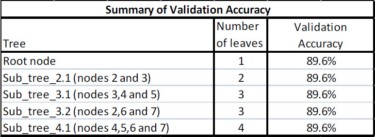
Table 4.5 shows the summary of the validation profits of all sub-trees and the tree:

Table 4.5

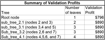
The optimal tree is sub-tree_2.1 with two leaves, because all the trees with equally high profits are trees of larger size. As you go down the columns “Number of leaves” and “Validation profit”, notice that, as the number of leaves increases, there is no increase in profit. Another way to think of this comparison with larger trees is to say that beyond sub-tree_2.1 the marginal profit = 0. That is, the incremental profit per additional leaf is zero. Hence sub-tree_2.1 is the optimum, or right-sized, tree. Note that sub-tree_4.1 is same as the maximal tree.

4.3.6 Average Profit vs. Total Profit for Comparing Trees of Different Sizes

In the above example I calculated the profit of a tree (or sub-tree) as the sum of the profits of its leaf nodes. The validation data has 5364 records, of which 560 are responders. Therefore average profit equals total profit divided by 5364. Since the denominator (number of records) is the same for all the trees compared, regardless of their number of leaves, I arrive at the same optimal tree using either average or total profits for comparison. Likewise, the sum of responders in all leaf nodes is equal to the total number of responders in the validation data set, which is 560 in this example. Hence calculating average profit as Total profit/560 for each (sub-)tree produces the same optimal tree.

4.3.7 Accuracy /Misclassification Criterion in Selecting the Right-sized Tree (Classification of Records and Nodes by Maximizing Accuracy)

Thus far, I have described how to classify each node and how to prune a tree using profit maximization as the criterion. Another often used criterion for both node classification and tree pruning is validation accuracy. In order to use this criterion for sub-tree selection or pruning in SAS Enterprise Miner, you must set the Assessment Measure property to Misclassification. Since misclassification rate = 1– validation accuracy, I use the terms validation accuracy and misclassification interchangeably.

When the Misclassification criterion is selected for assessment of the trees in pruning, the nodes are classified (assigned a target level) according to maximum posterior probability. This assignment is done during the training of the tree using the training data set.

4.3.7.1 Classification of the Nodes by Maximum Posterior Probability / Accuracy

This can be thought of as using a profit matrix of the following type:

Table 4.6

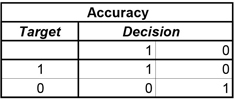
In this matrix, if a responder is correctly classified as a true responder, then one unit of accuracy is attained. If a non-responder is correctly classified as non-responder, then one unit of accuracy is gained. Otherwise, there is no gain.

As before, the nodes are classified as responder or non-responder nodes based on the posterior probabilities calculated from the training data set and the above profit matrix. In the root node of the training data set the proportion of responders is 9.9%, and the proportion of non-responders is 90.1%. Hence, if the root node is classified as a responder node, the accuracy would be 9.9%; if it is classified as non-responder node, the accuracy would be 90.1%. Hence, the optimal decision is to classify the root node as a non-responder node.

Similarly nodes 2, 3, 4, 5, 6, and 7 are all classified as non-responder nodes, since they all have more non-responders than responders.

4.3.7.2 Calculation of the Misclassification Rate / Accuracy Rate and Selection of the Right-sized Tree

Since the misclassification rate is 1 – validation accuracy, maximizing the validation accuracy is the same as minimizing the misclassification rate.

Table 4.7 shows the accuracy of the different sub-trees when applied to the validation data set. Using rules and partitioning definitions derived from the Training data set, all the nodes are classified as non-responder nodes. The tree has three sub-trees (not counting the root node as a tree): sub-tree_3.1 (with nodes 3, 4, and 5), sub-tree_3.2 (with nodes 2, 6, and 7), and sub-tree_2.1 (with nodes 2 and 3). The validation accuracy of sub-tree_3.1 = (2690+1004+1110)/5364 = 89.6%, and the misclassification rate is 10.4%. The validation accuracy of sub-tree_3.2 = (2114+1448+1242)/5364 = 89.6% and the corresponding misclassification rate is 10.4%. The validation accuracy of sub-tree_2.1 = (2114+2690)/5364 = 89.6%. The validation accuracy of the root node is (4804/5364) = 89.6%, and the misclassification rate is 10.4%. The validation accuracy of the maximal tree (with nodes 4, 5, 6, and 7) = (1004+1110+1448+1242)/5364= 89.6% with a misclassification rate of 10.4%. There is no gain in accuracy by going beyond the root node. Hence, the optimal or right-sized tree is a tree with the root node as its only leaf. As the number of leaves increased, there was no gain in accuracy.

Table 4.7

4.3.8 Assessment of a Tree or Sub-tree Using Average Square Error

When the target is continuous, the assessment of a tree is done using sums of squared errors. As in the case of a binary target, I use the validation data set to perform the assessment. Therefore, I begin by applying the node definitions or rules of partitioning developed using the training data set to the validation data set. The worth of a node is measured (inversely) by the Average Square Error for that node. For the $t^{t h}$ $t^{t h}$ node, the Average Square Error = $\frac{1}{n_{t}} \sum_{i = 1}^{n_{t}} (y_{i t} - {\bar{y}}_{t})^{2}$ $\frac{1}{n_{t}} \sum_{i = 1}^{n_{t}} (y_{i t} - {\bar{y}}_{t})^{2}$ , where $y_{i t}$ $y_{i t}$ is the actual value of the target variable for the $i^{t h}$ $i^{t h}$ record in the $t^{t h}$ $t^{t h}$ node, and ${\bar{y}}_{t}$ ${\bar{y}}_{t}$ is the expected value of the target for the $t^{t h}$ $t^{t h}$ node. The expected value ${\bar{y}}_{t}$ ${\bar{y}}_{t}$ is calculated from the Training data set, but the observations $y_{i t}$ $y_{i t}$ are from the Validation data set. The node definitions are constructed from the Training data set.

The overall Average Square Error for a tree or sub-tree is the weighted average of the average squared errors of the individual leaves, which can be given as follows:

\sum_{t = 1}^{T} \frac{n_{t}}{n} [\frac{1}{n_{t}} \sum_{i = 1}^{n_{t}} {(y_{i t} - {\bar{y}}_{t})}^{2}] .

$\sum_{t = 1}^{T} \frac{n_{t}}{n} [\frac{1}{n_{t}} \sum_{i = 1}^{n_{t}} {(y_{i t} - {\bar{y}}_{t})}^{2}] .$

Classification of nodes is not necessary for calculating the assessment value using Average Square Error (because the target in this case is continuous).

4.3.9 Selection of the Right-sized Tree

Display 4.5 gives another illustration of the selection of the right-sized tree from a sequence of optimal trees. In the graph shown in Display 4.5, the horizontal axis shows the number of leaves in each of the trees in the optimal sequence of trees. The vertical axis shows the average profit of each tree. The display clearly shows that the optimal tree has seven leaves. That is, a tree with seven leaf nodes has the same average validation profit as any tree with more leaves. Hence the tree with seven leaves is selected by the algorithm.

Display 4.5 shows the initially constructed maximal tree of size 14, before pruning it to a tree of size 7 using the technique described earlier.

Display 4.5

To get the Subtree Assessment plot as shown in Display 4.5, run the Decision Tree node as shown in Display 4.8 and open the Results window. Then click View →Model → Subtree Assessment Plot. A small chart window opens. Click on the down-arrow in the box located above the chart and select Average Profit. You will see a chart such as the one shown in Display 4.5. I used the profit matrix shown in Display 4.8 to calculate the average profit.

4.4 A Decision Tree Model to Predict Response to Direct Marketing

In this section, I develop a response model using the Decision Tree node. The model is based on simulated data representing the direct mail campaign of a hypothetical insurance company. The main purpose of this section is to show how to develop a response model using the Decision Tree node, and to make you familiar with the various components of the Results window.

Since this model predicts an individual’s response to direct mailing, it is called a response model. In this model, the target variable (the variable that I want to predict) is binary: it takes on values of response and no response.

The process flow diagram for this model is shown in Display 4.6.

Display 4.6

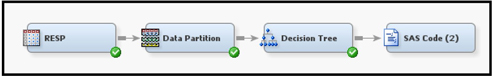
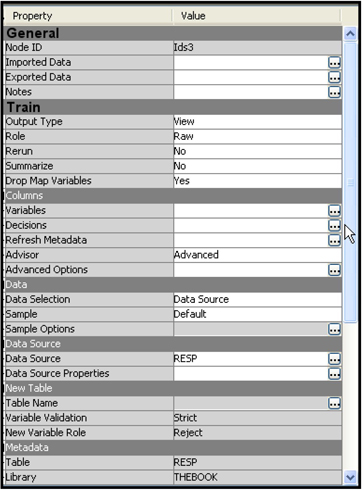
In the process flow diagram, the first node is the Input Data node. The properties of this node are shown in Display 4.7. You set the initial measurement levels of the variables by using the advanced settings of the Metadata Advisor Options. In this example, we are not overriding the initial settings of the variables. The role of the variable Resp, however, is changed to Target.

Display 4.7

I enter a profit matrix for the Decisions property of the Input Data node. This matrix is shown in Display 4.8. This matrix is used for making decisions about node classification and for making assessments of sub-trees.

Display 4.8

The next node is the Data Partition node. Display 4.9 shows the settings of the properties of this node.

Display 4.9

In this example, I allocated 60% of the data for training, 30% for validation, and 10% for testing. This allocation is quite arbitrary. You can use different proportions and then see how those proportions affect the results.

The third node in the process flow diagram is the Decision Tree node. The properties of the Decision Tree node are shown in Display 4.10.

Display 4.10

I kept the default values for all the properties. As a result, the nodes are split using the Chi-Square criterion. The threshold p-value for a split to be considered significant is set at 0.2. The sub-tree selection is done by comparing average profit since the Sub Tree Method property is set to Assessment, the Assessment Measure property is set to Decision, and a profit matrix is entered.

After running the Decision Tree node, you can open the Results window shown in Display 4.11.

Display 4.11

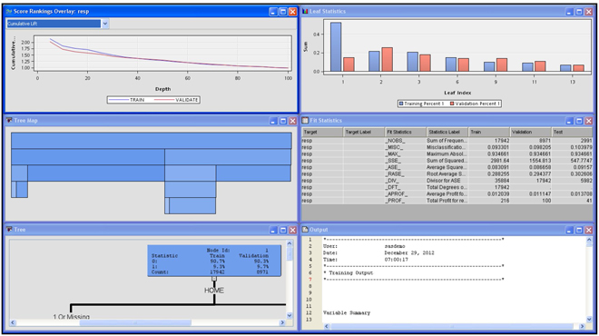
If you maximize the Tree pane in the Results window, you can see the tree as shown in Display 4.12.

Display 4.12

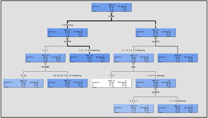
When you view the tree, the intensity of the color of the node indicates the response rate of the customers included in the node. In the tree above, Node 12 has a white background (least intensity of color), which indicates the highest response rate (in the Training data set). The customers in this node do not own a home (HOME= 0), they own one or more credit cards (NUMTR=1, 2, 3, 4, 6, 7) and they are young (AGE > 22.5). This node also includes those customers with missing values for the variable NUMTR.

The Cumulative Lift chart is shown in the Score Rankings Overlay pane in the top left-hand section of the Results window. To see a list of the available charts, click the arrow on the box where the chart type is displayed.

An alternative way of making charts is through the Data Options Dialog window. Open this window by right-clicking in the chart area, and selecting Data Options. The Data Options Dialog window is shown in Display 4.13.

Display 4.13

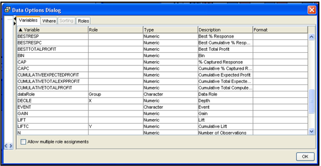
In Display 4.13, there is an X in the Role column of the variable DECILE, and Y in the Role column of the variable LIFTC. This means that the decile ranking is shown on the X-axis (horizontal axis) and the cumulative lift is shown on the Y axis. With these settings, you get the lift chart shown in the Score Rankings pane in Display 4.11. When you select different variables for the X and Y axes, you can get different charts. To make this selection, click on the Role column corresponding to a variable, and select the role. For example, by setting the Role of the variable CAPC to Y and the Role of DECILE to X, I get a Cumulative Captured Response chart, as shown in Display 4.14.

Display 4.14

According to this chart, if I target the top 40% of the customers ranked by the predicted probability of response, then I will capture 54.7% percent of all responders. These capture rates are not impressive, but they are sufficient for demonstrating the tool.

To get a view of the pruning process displayed by the Subtree Assessment plot, select View→Model→ Subtree Assessment Plot in the Results window, as shown in Display 4.15.

Display 4.15

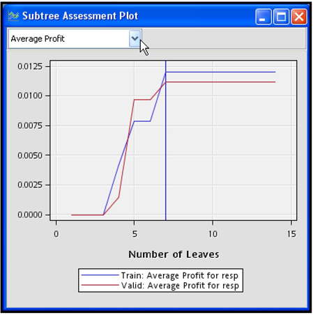
The plot generated by choosing the settings in Display 4.15 is shown in Display 4.16.

Display 4.16

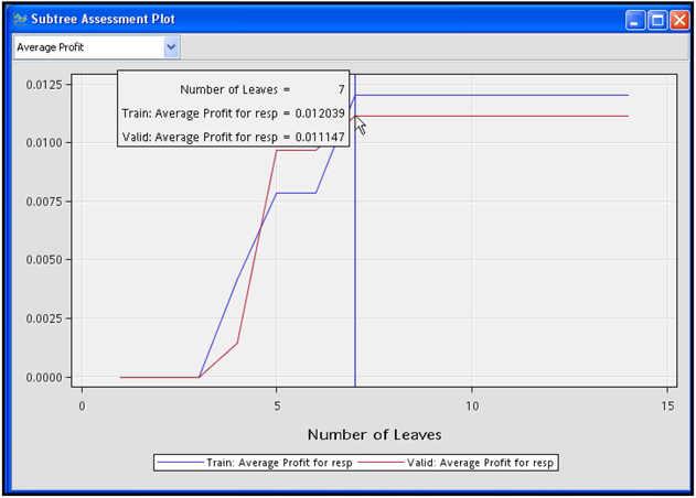
Display 4.16 shows the average profit for trees of different sizes. On the horizontal axis, the number of leaves is shown indicating the size of the tree. On the vertical axis, the average profit of the tree is shown. The calculation of the average profit is illustrated in Section 4.2.5 and in Step 2 of Section 4.3.5.

The graph shown in Display 4.16 depicts the pruning process. An initial tree with 14 leaves is grown with the training data set, and a sub-tree of only 7 leaves is selected using the validation data set. The selected tree is shown in Display 4.12.

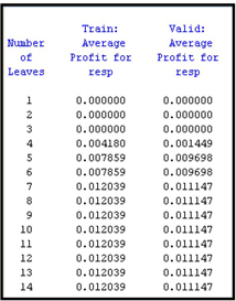
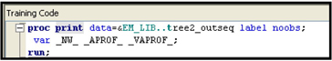
The data behind these charts can be retrieved by clicking the Table icon on the toolbar in the Results window. The data is stored in a SAS data set in the project directory. Output 4.1 is printed from the saved data set, and it shows the data underlying the graph shown in Display 4.16. The SAS code shown in Display 4.17 is run from the SAS code node for generating Output 4.1.

Output 4.1

Display 4.17

Output 4.1 and the graph in Display 4.16 show that the average profit reached its maximum at seven leaves for both the Validation data and Training data. This may not always be the case. The Decision Tree node selects the right-sized tree based on validation profits only.

Display 4.18 shows a partial list of the score code.

Display 4.18

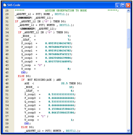
The segment of the code included in Display 4.18 shows how an observation is assigned to Leaf Node 7. Note that P_resp1 = 0.09239130434782 is computed from the Training data set and it is called the posterior probability of response. P_resp0 = 0.90760869565217 is also computed from the Training data set. It is called the posterior probability of non-response. These posterior probabilities are the same as ${\hat{P}}_{1}$ ${\hat{P}}_{1}$ and ${\hat{P}}_{0}$ ${\hat{P}}_{0}$ discussed in Section 4.2.2. Any observation that meets the definition of Leaf Node 1 is assigned these posterior probabilities. This, in essence, is how a decision tree model predicts the probability of response. This code can be applied to score the target population, as long as the data records in the prospect data set are consistent with the sample used for developing the model. Display 4.19 shows another segment of the score code, which shows the decision-making process in classifying customers as responders or non-responders.

Display 4.19

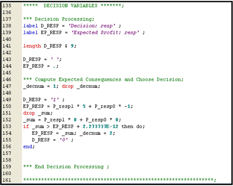
This code shows how decisions are made with regard to assigning an observation to a target level (such as response and non-response). The decision-making process is also discussed in Section 4.2.2 and Step 1C of Section 4.3.5.

The decision process is clear from the code segments in Displays 4.18 and 4.19. In any data set, an observation is assigned to a node first, as shown in Display 4.18. Then, based on the posterior probabilities (P_resp1 and P_resp0) of the assigned node and the profit matrix, expected profits are computed under Decision1 and Decision2. The expected profit under Decision1 is given by the SAS statement EP_RESP = P_resp1*5 + p_resp0*(-1). Note that the numbers 5 and -1 are from the first column of the profit matrix. If you classify a true responder as a responder, then you make a profit of $5, and if you classify a non-responder as a responder, the profit is -$1.0. Hence, EP_RESP represents the consequences of classifying an observation as a responder. The alternative decision is to classify an observation as a non-responder, and this is given by the SAS statement _sum = P_resp1*0 + P_resp0* 0. The two numbers 0 and 0 are the second column of the profit matrix. The code shows that if _sum > EP_RESP, then the decision is to assign the target level 0 to the observation. The variable that indicates the decision is D_RESP, which takes the value 0 if the observation is assigned to the target level 0, or 1 if the observation is assigned to the target level 1. Since observations that are assigned to the same node will all have the same posterior probabilities, they are all assigned the same target level.

4.4.1 Testing Model Performance with a Test Data Set

I used the Training data set for developing the node definitions and posterior probabilities, and I used the Validation data set for pruning the tree to find the optimal tree. Now I need an independent data set on which to evaluate the model. The test data set is set aside for this assessment. I connect the Model Comparison node to the Decision Tree node and run it. The Results window of the Model Comparison node shows the lift charts for all three data sets. These charts are shown in Display 4.20.

Display 4.20

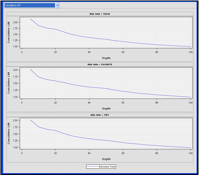
The performance of the model on the test data is very similar to its performance on the Training and Validation data sets. This comparison shows that the model is robust.

4.4.2 Applying the Decision Tree Model to Score a Data Set

This section shows the application of the decision tree model developed earlier to score a prospect data set. The records in the prospect data set do not have the value of the target variable. The target variable has two levels, response and no response. I use the model to predict the probability of response for each record in the prospect data set.

I use the Score node to apply the model and make the predictions. I add an Input Data node for the prospect data and a Score node in the process flow, as shown in Display 4.21.

Display 4.21

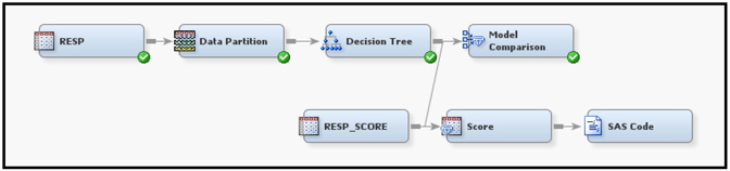
In Display 4.21, the data set that is being scored is named RESP_SCORE, and its role is set to Score. When the Score node is run, it applies the Decision Tree model to the data set RESP_SCORE, generates predictions of the target levels and their probabilities, and creates a new data set by appending the predictions to the prospect data set. Output 4.2 shows the appended variables in the new data set.

Output 4.2

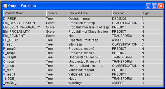
The predicted probabilities are P_resp1 and P_resp0. These are the posterior probabilities created in the training process. They are part of the Decision Tree model. The Score node gives the predicted values of the target levels, based on profit maximization. These predicted values are stored as the variable D_RESP. Display 4.22 shows the frequency distribution of the predicted target levels, based on profit maximization.

Display 4.22

Display 4.22 shows that, under profit maximization, 1113 out of the total 29904 customers are designated as responders. The remaining 28791 customers are designated as non-responders. The score code gives an alternative prediction of the target levels based on predicted probability (which is the same as the posterior probability).

If predicted probability of non-response is greater than the predicted probability of response for any record, then the variable EM_Classification is given the value 0 for that record. If the predicted probability of response is greater than the predicted probability of non-response for a given record, then the variable EM_Classification for that record is given the value 1. Thus, the variable EM_Classification indicates whether a record is designated as a responder or a non-responder record. Display 4.23 shows that, in the data set, the variable EM_Classification takes the value 0 for 29873 records, and it takes the value 1 for 31 records. Thus, according to the decisions based on error minimization, only 31 customers (records) are designated as responders, while 29867 customers are designated as non-responders.

The frequency distribution of EM_Classification is shown in Display 4.23.

Display 4.23

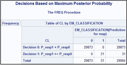
The program that generated Displays 4.22 and 4.23 is shown in Display 4.24. It was run in the SAS code node.

Display 4.24

Displays 4.25A and 4.25B show segments of the Flow code generated by the Score node, which shows how the E_RESP and EM_Classification are calculated. To see the Flow code, click Score node → Results → SAS Results → Flow Code. By scrolling down in this window, you can see the code shown in Displays 4.25A and 4.25B.

Display 4.25A

Display 4.25B

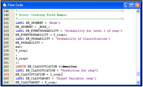
4.5 Developing a Regression Tree Model to Predict Risk

In this section, I develop a decision tree model to predict risk. In general, risk is defined as the expected amount of loss to the company. An auto insurance company incurs losses resulting from such events as accidents or thefts. An auto insurance company is often interested in predicting the expected loss frequency of its customers or prospects. The insurance company can set the premium for a customer according to the predicted loss frequency. Loss frequency is measured as the number of losses per car year, where car year is defined as the duration of the insurance policy multiplied by the number of cars insured under the policy. If the insurance policy has been in effect for four months and one car is covered, then the number of car years is 0.3333. If there is one loss during this four months then the loss frequency is 1/ (4/12) = 3. If, during these four months, two cars are covered under the same policy, then the number of car years is 0.6666; and if there is one loss, the loss frequency is 1.5.

The target variable in this model is the LOSSFRQ (loss frequency), which is continuous. When the target variable is continuous, the tree constructed is called a regression tree. A regression tree, like a decision tree, partitions the records (customers) into segments or nodes. The regression tree model consists of the leaf nodes. While posterior probabilities are calculated for each leaf node in a decision tree model, the expected value or mean of the target variable is calculated for each leaf node in a regression tree model. In the current example, the Tree calculates the expected frequency of losses for each leaf node or segment. These target means are calculated from the training data.

The process flow for modeling risk is shown in Display 4.26.

Display 4.26

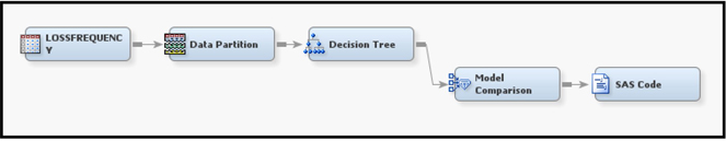
In this example, the data source is created from the SAS table called LossFrequency, and I used Advanced Metadata Options. I set the Class Levels Count Threshold to 5.

In this example, the modeling data set is partitioned such that 60% of the records are allocated for training, 30% for validation, and 10% for testing. The selection method used for this partitioning is simple random sampling.

The property settings of the Decision Tree node are shown in Display 4.27.

Display 4.27

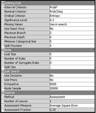
The main difference between trees with binary targets and trees with continuous targets is in the test statistics used for evaluating the splits and the calculation of the worth of the trees. For the continuous target, the test statistic has an F-distribution. The model assessment is done by using the Error Sums of Squares. The Splitting Rule Interval Criterion property is ProbF, which is default for interval targets. The Assessment Measure property for assessment is set to Average Square Error. Section 4.3.1.4 discusses the ProbF criterion for calculating the worth of a split. Section 4.3.8 discusses how Average Square Error is calculated.

Displays 4.28A through 4.28C show the Tree model developed by the Decision Tree node.

Display 4.28A

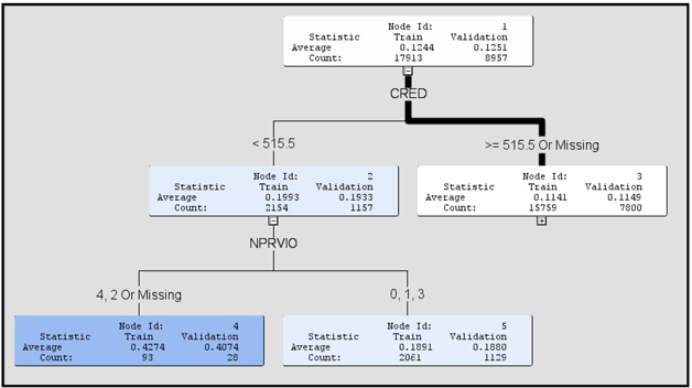
Display 4.28B

Display 4.28C

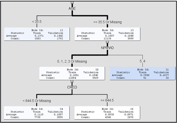
The variables defining the nodes of the tree are NPRVIO (number of prior violations), CRED (Credit score), and AGE (Age).

Display 4.29, which is generated by the Model Comparison node, shows the mean of predicted loss frequency in the Training, Validation and Test data sets. You need to compare the predicted means with the actual means to assess how well the model succeeds in ranking the various risk groups. Displays 4.29A, 4.29B and 4.29C show the actual and predicted mean of the target variable (Loss Frequency) by percentile for the Training, Validation, and Test data sets.

Display 4.29

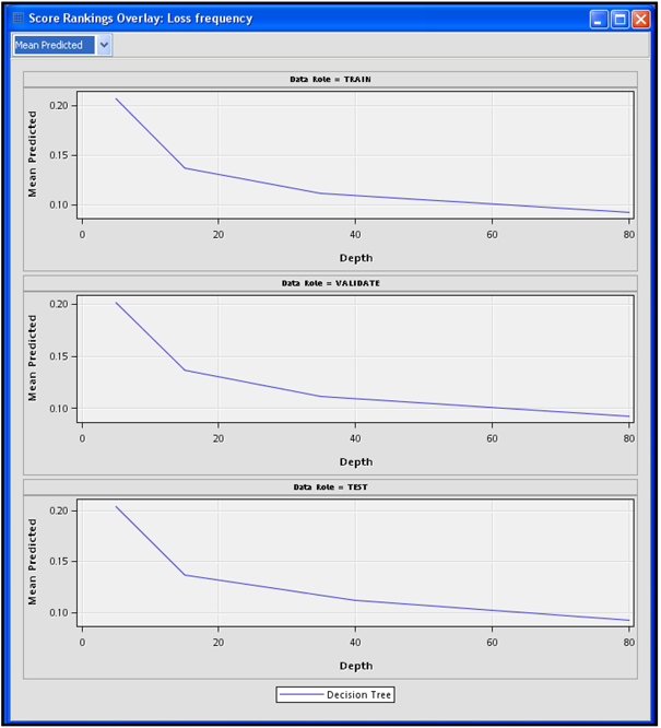
The percentiles computed from ordered values of the predicted loss frequency are shown on the horizontal axis, with those customers with the highest loss frequency in the first percentile and those with the lowest losses in the tenth percentile. The vertical axis shows the mean of predicted loss frequency for each percentile.

Display 4.29A

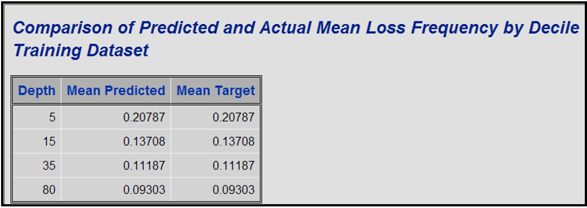
Display 4.29B

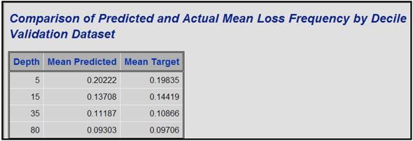
Display 4.29C

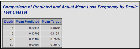
Displays 4.29A to 4.29C show that, for the Training, Validation and Test data sets, the mean of the actual loss frequency (Mean Target) is highest for the 5^th percentile, the mean of the actual loss frequency for the 15^th percentile is lower than that of the 5^th percentile, the mean of the actual loss frequency for the 40^th percentile is lower than that of the 15^th percentile, etc. The pattern of Mean Target exhibited in Displays 4.29A to 4.29C shows that the model is rating the risk groups correctly.

To generate the tables presented in Displays 4.29A to 4.29C, you can go to the Code Editor window of the SAS Code node, type in SAS code similar to the code in Display 4.29D, and run it.

Display 4.29D

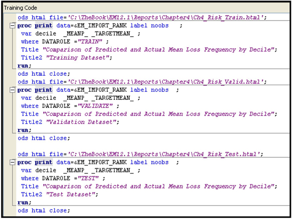
You can see a plot of the actual and predicted means for the training and validation data sets in the Results window of the Decision Tree Node .

4.5.1 Summary of the Regression Tree Model to Predict Risk

Although the regression tree shown in Displays 4.28A-4.28C is developed from simulated data, it provides a realistic illustration of how this method can be used to identify the profiles of high-risk groups.

We used the regression tree model developed in this section to group the records (in this case, the customers) in the data set into seven disjoint groups—one for each of the seven leaf nodes or terminal nodes on the tree—as shown in Display 4.30. The tree model also reports the mean of the target variable for each group, calculated from the Training data set. In this example, these means are used as predictions of the target variable loss frequency for each of the ten groups. Since the mean of the target variable for each group can be used for prediction, I refer to it as Predicted Loss Frequency in Display 4.30. The predicted loss frequency of a group reflects the level of risk associated with the group. The groups are shown in decreasing order of their risk levels. Display 4.30 also shows the profiles of the different risk groups, that is, their characteristics with regard to previous violations, credit score, and age.

Display 4.30

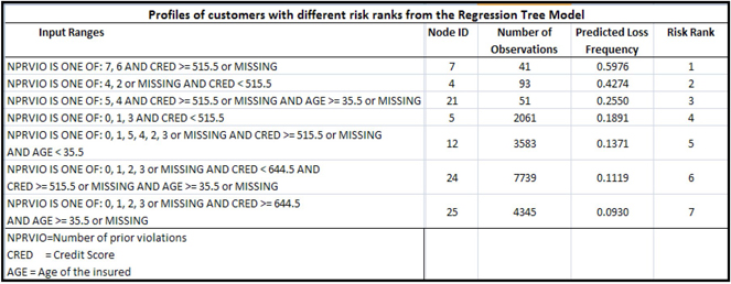
In an effort to prevent unfair or discriminatory practices by insurance companies, many state agencies that oversee the insurance industry have decreed that certain variables cannot be used for risk rating, rate setting, or both. The variables that appear in Display 4.30 are not necessarily legally permitted variables. The table is given only for illustrating the Regression Tree model.

4.6 Developing Decision Trees Interactively

You can develop decision and regression trees either autonomously or interactively. We developed autonomous trees in Sections 4.4 and 4.5. In this section, I show how to develop decision trees interactively. You can use the Interactive property of the Decision Tree node either to modify a tree that was developed previously or to develop an entire tree starting from the root node. To demonstrate the Interactive facility of the Decision Tree node, I created the process flow diagram shown in Display 4.31. This process flow diagram includes three instances of the Decision Tree node. I use the first instance of the Decision Tree node, denoted by ①, to demonstrate how to modify a previously created tree in interactive mode. I use the second instance of the Decision Tree node, denoted by ②, to develop an entire tree interactively starting from the root node. Finally, I use the Decision Tree node denoted by ③ to develop a maximal tree in an interactive mode. The size of the maximal tree is controlled by the values of the Significance Level, Maximum Depth, Leaf Size, and Split Adjustment properties.

Display 4.31

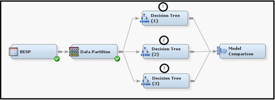
4.6.1 Interactively Modifying an Existing Decision Tree

I first created a tree autonomously by running the Decision Tree node ① located at the top of the process flow diagram. The resulting tree is shown in Display 4.32.

Display 4.32

I switched to the interactive mode by clicking located at the right of the Interactive property of the Decision Tree node, as shown in Display 4.33.

Display 4.33

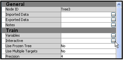
The Interactive Tree window opens with the tree that was autonomously created, shown in Display 4.34.

Display 4.34

4.6.1.1. Changing the Split Point of an Interval-Scaled Variable

To modify this tree, select the node whose definitions you want to change, as shown by the mouse-pointer in Display 4.34. In this example, I select Node 4 (see Display 4.32) for modification. You can see in Display 4.32 that this node is split by using the AGE variable, with the split point at 22.5 years. To change the split point for this node (the terms split point and split value are used interchangeably) to some other value, right-click on Node 4 and select Split Node, as shown in Display 4.35.

Display 4.35

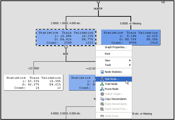
A window with information about the logworth of the variables appears, as shown in Display 4.36.

Display 4.36

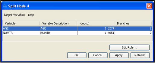
The AGE variable has a logworth of 1.8274. Since it has the highest logworth of any input variable listed in Display 4.36, it was chosen for splitting the node, and the node was split at 22.5 years of age. To change the split points, click Edit Rule. The Split Rule window opens, as shown in Display 4.37.

Display 4.37

Type the new split value (24.5) in the New split point box and click Add Branch. A new branch 3 is added, as shown in Display 4.38. To remove the old split point, highlight branch 1and click Remove Branch. The branches are renumbered so that 2 and 3 are now 1 and 2, respectively. The split rule is changed.

Display 4.38

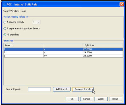
Click Apply, and then click OK. Close the Split Node window by clicking OK. The logworth of the new split value is calculated, which is shown in Display 4.39.

Display 4.39

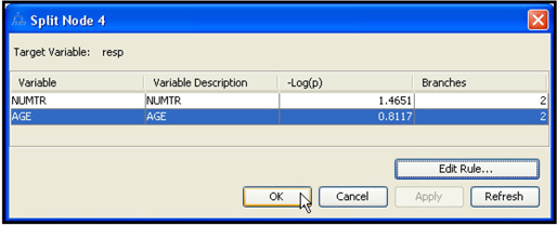
By comparing Displays 4.36 and 4.39, you can see that the logworth of the new split point on the AGE variable is smaller than that of the original split value. This is not surprising because the original split value selected by the tree algorithm was the best one. Any arbitrary split points other than the one selected by the SAS Enterprise Miner Tree algorithm tends to have a smaller logworth. Click OK as shown in Display 4.39. The node definition is modified as shown in Display 4.40. (The modified node is outlined in dashed lines in Display 4.40.)

Display 4.40

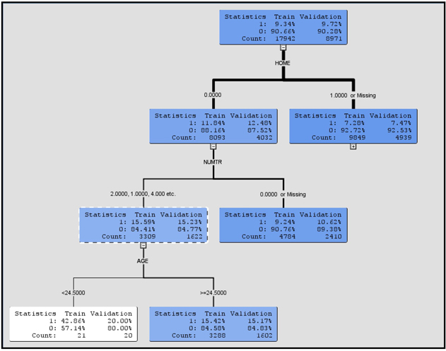
To further split the node with age >=24.5, right-click on it and select Train Node from the menu. The node is split, as shown in Display 4.41.

Display 4.41

Close the Interactive Tree window by clicking the X in the top right-hand corner and open the Results window where the interactively created tree appears as shown in Display 4.42.

Display 4.42

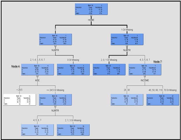
By comparing the tree in Display 4.42 with the tree in Display 4.32, you see that we have successfully changed the point at which Node 4 is split. The change we have made is trivial, but it is sufficient to demonstrate how to modify the node definitions of an existing tree.

4.6.1.2 Changing the Split Point of a Nominal (Categorical) Variable

In the preceding example, we changed the split value of the variable AGE, which is an interval scaled variable. In order to show how to change the split value of a nominal variable, I now use the INCOME variable as an example and change the definition of Node 7 of the tree shown in Display 4.42

To open the tree in an interactive mode, click located at the right of the Interactive property of the Decision Tree node ① as shown in Display 4.33. The Interactive Tree window opens with the tree we modified in the previous section (see Display 4.42).

Right click on Node 7, and select Split Node from the menu, as shown in Display 4.43.

Display 4.43

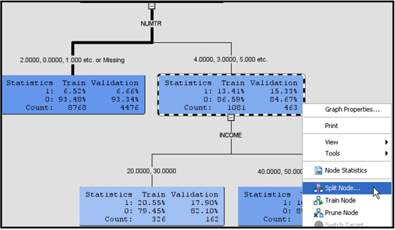
A window showing the logworth of the inputs considered for splitting Node 7 appears, as shown in Display 4.44.

Display 4.44

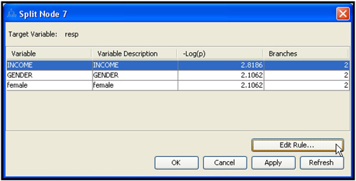
Since the INCOME variable is used for splitting Node 7, it is highlighted. Click Edit Rule. The Split Rule window opens.

Just for illustration, we assign the value 40 to Branch 1. To do this, click on the row corresponding to value 40, enter 1 in the Assign to branch box, and click Assign, as shown in Display 4.45.

Display 4.45

The split rule is changed as shown in Display 4.46.

Display 4.46

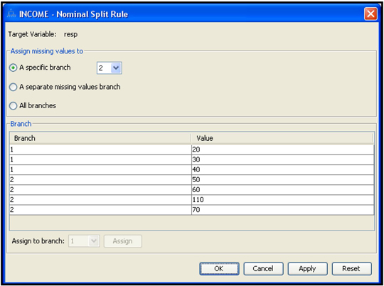
Click Apply, and then click OK. Close the Split Node window by clicking OK. The logworth at the new split point appears in the logworth table, as shown in Display 4.47.

Display 4.47

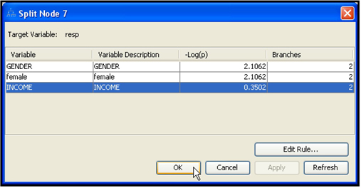
From Display 4.47 it is clear that the logworth of INCOME variable with the new split value is smaller than the split value that was originally selected by the Decision Tree node. The logworth of an arbitrary split point is in general less than that of the statistically optimal split point selected by the Decision Tree algorithm.

If you click OK, the modified tree appears, as shown in Display 4.48.

Display 4.48

Close the Interactive Tree by clicking on the X in the top right-hand corner of the window. Open the Results window of the Decision Tree node. The modified tree now appears in the Results window, as shown in Display 4.49.

Display 4.49

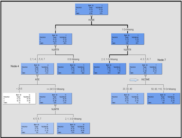
Compare Display 4.49 with Display 4.42 to confirm that Node 7 is split at a new value of income.

In general, arbitrary constraints diminish the predictive performance of any model, and a Decision Tree model is no exception. In real life, either for marketing convenience or other business reasons, you must impose constraints on a model. I leave it to you to compare the original autonomous tree and the modified tree with respect to such measures as lift and cumulative lift, etc. from the Results window.

4.6.2 Growing a Tree Interactively Starting from the Root Node

In this section we grow a tree starting from the root node. Click the Decision Tree node ② shown in Display 4.31. In the Properties panel, click located to the right of the Interactive property. The Interactive window opens, as shown in Display 4.50.

Display 4.50

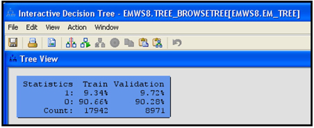
At this point the tree has only the root node. To split the root node into two child nodes, right-click on it and select Split Node. The Split Node window opens, as shown in Display 4.51.

Display 4.51

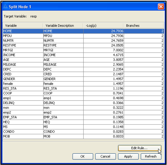
Each variable has a number of candidate split points. The algorithm first selects the best split point of each variable. The logworth of the selected best split point for each variable is listed in the table in Display 4.51. Next, the algorithm selects the best split point on the best variable. The best variable is the one that has the highest logworth at its best split point. In this example, both the variables HOME and MFDU are the best variables, because they have the same logworth at their respective best split points, but the algorithm selected the variable HOME for splitting the node. To see exactly what the best of the best split points is, click Edit Rule. The Split Rule window opens, as shown in Display 4.52.

Display 4.52

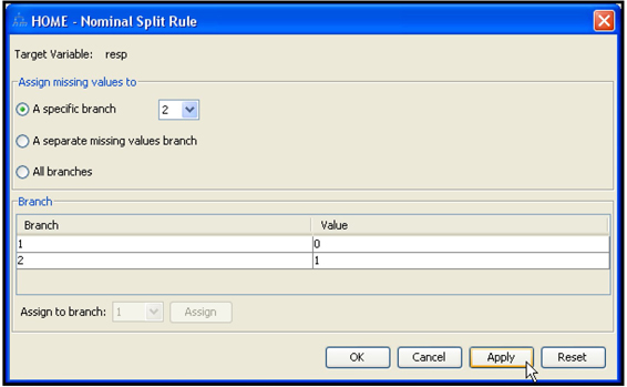
Display 4.52 shows that the variable HOME takes on the value 0 or 1, 0 indicating that the customer is a renter and 1 indicating the customer is a home owner. The node is split in such a way that all customers with HOME = 0 are placed into the left branch (branch 1) and those with HOME =1 are placed in the right branch (branch 2). By default, customers with missing values of the variable HOME are placed in branch 2. You can change this rule by changing the value next to A specific branch to 1. You may also choose to assign the records with missing values to a separate branch or distribute them to all branches. In this example, I am leaving the default assignment of the observations with missing values to branch 2. Then I click Apply, and then OK. Close the Split Node window by clicking OK. A tree is grown with two branches, as shown in Display 4.53.

Display 4.53

The variable HOME stands for home ownership status. It indicates the type of home a customer owns. MFDU indicates whether a customer lives in a multi-family dwelling unit. These two variables are very similar, hence they have the same logworth. In parametric models such as the Logistic Regression model, the inclusion of both these variables would have resulted in unstable estimates of the coefficients or other undesirable results due to collinearity. But in the case of decision trees, collinearity is not a problem.

To grow a larger tree by adding more splits, select the node that is at the bottom left of the tree in Display 4.53, right-click on it and select Split Node as we did before.

The Split node window opens, as shown in Display 4.54.

Display 4.54

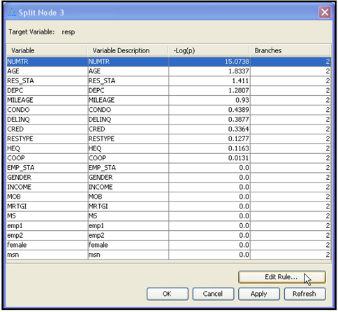
The best variable for splitting Node 3 is NUMTR, which indicates the number of credit cards a customer has. You can select another variable for splitting. Although the next best variable is AGE, the logworth of the best split on the AGE variable is only 1.8337, which is much smaller than the logworth of the variable NUMTR. So we accept the variable selected (NUMTR) by the tree algorithm. To see the split point selected by the algorithm, click Edit Rule. The Split Rule window opens, as shown in Display 4.55.

Display 4.55

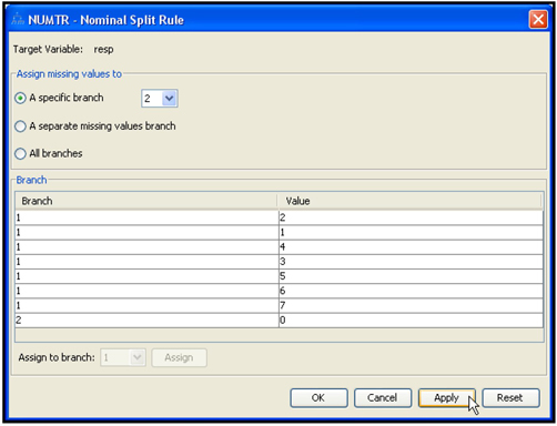
Since I do not have any particular reason for changing the split values selected by the algorithm (see Display 4.55), I click Apply and OK. Display 4.56 shows the expanded tree.

Display 4.56

Now let us split the second branch (right-hand side) from the root node. Right-click on this node and select Split Node from the menu.

Display 4.57 shows all the inputs available for splitting this node and the logworth of the best split point for each of them.

Display 4.57

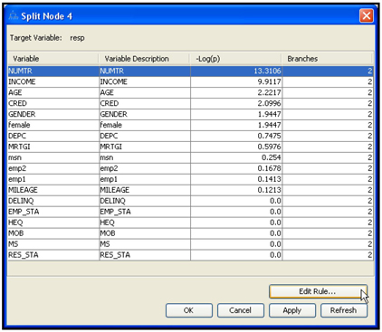
As Display 4.57 shows, the statistically best variable is NUMTR. The second best variable is INCOME. For purposes of illustration, we override the statistically best variable NUMTR with the second best variable INCOME by selecting it and clicking Edit Rule. Display 4.58 shows the new split rule.

Display 4.58

According to this split rule, the records with INCOME less than or equal to $30,000 are sent to Branch 1, and those with income greater than $30,000 are sent to Branch 2. To accept this split rule, click Apply and OK. Close the Split Node window by clicking OK. The resulting tree is shown in Display 4.59.

Display 4.59

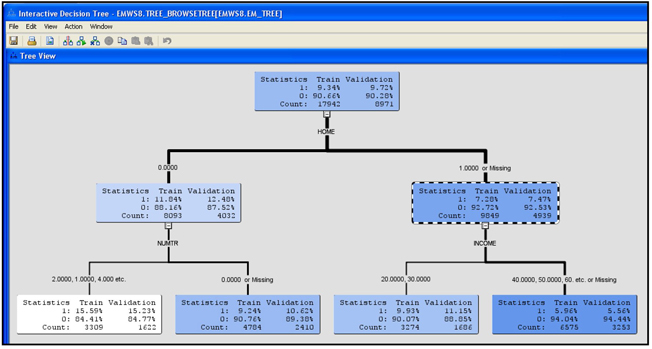
Close the Interactive Decision Tree window by clicking the X in the top right-hand corner of the window. Next, right-click on the Decision Tree node indicated by ② in the process flow diagram shown in Display 4.31, select Results, and expand the Tree sub-window. The Tree that we have grown interactively appears, as shown in Display 4.60.

Display 4.60

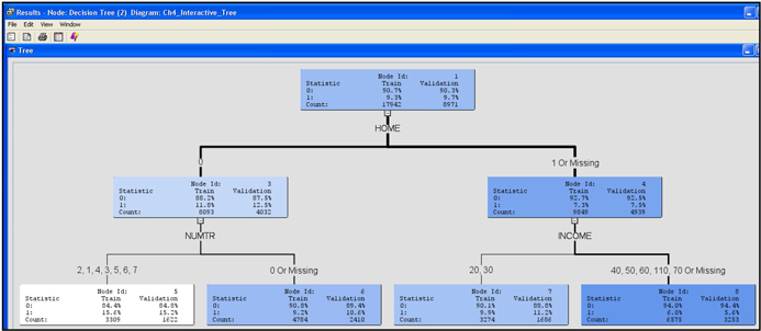
4.6.3 Developing the Maximal Tree in Interactive Mode

In this section, we grow a maximal tree starting from the root node. The maximal tree is the largest tree that can be grown, subject to the stopping rules defined by the Decision Tree properties, which were discussed earlier. Select the Decision Tree node ③ shown in Display 4.31 by clicking on it. In the Properties panel, click located to the right of the Interactive property. The Interactive window opens showing a tree with only the root node. Right click on the root node, and select Train Node, as shown in Display 4.61.

Display 4.61

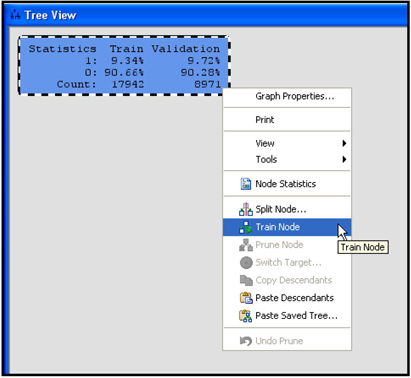
The maximal tree is created. Since the tree is too large, I am not including it here. Instead I include the Subtree Assessment plot. To view the Subtree Assessment plot, click View on the menu bar, and select Subtree Assessment Plot. The plot is shown in Display 4.62.

Display 4.62

As you can see from Display 4.62, the average profit does not increase with the number of leaves beyond seven leaves. Hence the optimal tree is the one with seven leaves, or terminal nodes. Close the Interactive Tree window.

Run the Model Comparison node to compare the three trees we created in Sections 4.6.1, 4.6.2, and 4.6.3. Display 4.63 shows the ROC charts for these three trees.

Display 4.63

Display 4.63 shows that the maximal tree performs slightly better than Decision Trees 1 and 2, on the basis of the ROC curves constructed from the Training data. But when we compare the ROC curves constructed from the Validation and Test data sets, the maximal tree performs no better than the other trees.

4.7 Summary

• Growing a decision tree means arriving at certain rules for segmenting a given data set, stated in terms of ranges of values for inputs, and assigning a target class³ (such as response or non-response) to each segment that is created.

• The Training data set is used for developing the rules for the segmentation, for calculating the posterior probabilities of each segment (or the target mean of each segment when the target variable is continuous), and for assigning each segment to a target class when the target is categorical.

• Node definitions, target means, posterior probabilities, and the assignment of the target levels to nodes do not change when the tree is applied to the Validation, or Prospect, data set.

• SAS Enterprise Miner offers several criteria for splitting a node; you can select the criterion suitable for the type of model being developed by setting the Splitting Rule Criterion property to an appropriate value.

• In general, there are a number of sub-trees within the initial tree that you need to examine during the tree development. The Training data set is used to create this initial tree, while the Validation data set is used to select the best sub-tree by applying an assessment measure that you choose. Several measures of assessment are available in SAS Enterprise Miner, and you can select one of them by setting the Sub-tree Assessment Measure property to a certain value. Selecting the best sub-tree is often referred to as pruning.

• SAS Enterprise Miner offers different methods for selecting a sub-tree: instead of applying an assessment measure to select a sub-tree, you can also select the tree with the maximum number of leaves, or the one with a specified number of leaves (regardless of whether the tree has maximum profit, or minimum cost, or meets any other criterion of assessment.)

• A decision tree model consists finally of only the leaf nodes (also known as the terminal nodes) of the selected tree, the attributes of which can be used for scoring prospect data, etc.

• The definition of the leaf nodes, the target classes assigned to the nodes, and their posterior probabilities can all be seen in the SAS code (score code) generated by SAS Enterprise Miner. You can export the SAS code if the scoring is to be applied to external data.

• The two models developed in this chapter, one for a binary target and one for a continuous target, serve as examples of how to use the Decision Tree node: how to interpret the results given in the Output window and how to interpret the various types of graphs and tables associated with each of them.

• The Regression Tree model developed for predicting risk is used to rank the customers according to their degree of risk. Each risk group is then profiled and represented as an exclusive segment of the tree model.

• You can develop decision trees interactively in SAS Enterprise Miner. You can modify a previously developed tree or grow a whole tree interactively, starting from the root node. You can also grow a maximal tree interactively.

4.8 Appendix to Chapter 4

4.8.1 Pearson’s Chi-Square Test

As an illustration of the Chi-square test, consider a simple example. Suppose there are 100 cases in the parent node ( $τ$ $τ$ ), of which 10 are responders and 90 are non-responders. Suppose this node is split into two child nodes, A and B. Let A have 50 cases, and let B have 50 cases. Also, suppose there are 9 responders in child node A, and there is 1 responder in child node B. The parent node has 10 responders and 90 non-responders.

Here is a 2 x 2 contingency table representing the split of parent node τ:

	Child node A	Child node B
Responders	9	1
Non-responders	41	49

The null hypothesis is that the child nodes A and B are not different from their parent node in terms of class composition (i.e., their mix of responders and non-responders). Under the null hypothesis, each child node is similar to the parent node, and contains 10% responders and 90% non-responders.

Expected frequencies under the null hypothesis are as follows:

	Child node A	Child node B
Responders	5	5
Non-responders	45	45

χ^{2} = \sum \frac{{(O - E)}^{2}}{E} = \frac{{(4)}^{2}}{5} + \frac{{(- 4)}^{2}}{45} + \frac{{(- 4)}^{2}}{5} + \frac{{(4)}^{2}}{45} = 7.1

$χ^{2} = \sum \frac{{(O - E)}^{2}}{E} = \frac{{(4)}^{2}}{5} + \frac{{(- 4)}^{2}}{45} + \frac{{(- 4)}^{2}}{5} + \frac{{(4)}^{2}}{45} = 7.1$

A Chi-square value of 7.1 implies the following values for p-value and for logworth:

p-value = 0.00766 and logworth = ${log}_{10} (p -value) = 2 .11546 .$ ${log}_{10} (p -value) = 2 .11546 .$

The pvalue is the probability of the Chi_Square statistic taking a value of 7.1 or higher when there is no difference in the child nodes. In this case it is very small, 0.00766. This indicates that in this case, the child nodes do differ significantly with respect to their composition of responders and non-responders.

4.8.2 Adjusting the Predicted Probabilities for Over-sampling

When modeling rare events, it is a common practice to include all the records having the rare event, but only a fraction of the non-event records in the modeling sample. This practice is often referred to as over-sampling, case-control sampling, or biased sampling.

For example, in response modeling, if the response rate is very low, you can include in the modeling sample all the responders available and only a randomly selected fraction of non-responders. The bias introduced by such over-sampling is corrected by adjusting the predicted probabilities with prior probabilities. Display 2.15 in Chapter 2 shows how to enter the prior probabilities.

Adjustment of the predicted probabilities can be illustrated by a simple example. Suppose, based on a biased sample, the unadjusted probabilities of response and no-response calculated by the decision tree process for a particular node $T$ $T$ are ${\hat{P}}_{1 T}$ ${\hat{P}}_{1 T}$ and ${\hat{P}}_{0 T}$ ${\hat{P}}_{0 T}$ . If the prior probabilities, that is, the proportion of responders and non-responders in the entire population, are known to be $π_{1} and π_{0}$ $π_{1} and π_{0}$ , and if the proportion of responders and the non-responders in the biased sample are $ρ_{1}$ $ρ_{1}$ and $ρ_{0}$ $ρ_{0}$ , respectively, then the adjusted predictions of the probabilities are given by

P_{1 T} = \frac{{\hat{P}}_{1 T} (π_{1} / ρ_{1})}{{\hat{P}}_{0 T} (π_{0} / ρ_{0}) + {\hat{P}}_{1 T} (π_{1} / ρ_{1})}, and

$P_{1 T} = \frac{{\hat{P}}_{1 T} (π_{1} / ρ_{1})}{{\hat{P}}_{0 T} (π_{0} / ρ_{0}) + {\hat{P}}_{1 T} (π_{1} / ρ_{1})}, and$

P_{0 T} = \frac{{\hat{P}}_{0 T} (π_{0} / ρ_{0})}{{\hat{P}}_{0 T} (π_{0} / ρ_{0}) + {\hat{P}}_{1 T} (π_{1} / ρ_{1})},

$P_{0 T} = \frac{{\hat{P}}_{0 T} (π_{0} / ρ_{0})}{{\hat{P}}_{0 T} (π_{0} / ρ_{0}) + {\hat{P}}_{1 T} (π_{1} / ρ_{1})},$

where $P_{1 T}$ $P_{1 T}$ is the adjusted probability of response, and $P_{0 T}$ $P_{0 T}$ is the adjusted probability of no-response. It can be easily verified that $P_{1 T} + P_{0 T} = 1$ $P_{1 T} + P_{0 T} = 1$ . If there are $n_{1 T}$ $n_{1 T}$ responders and $n_{o T}$ $n_{o T}$ non-responders in node $T$ $T$ , prior to adjustment, then the adjusted number of responders and non-responders will be $(\frac{π_{1}}{ρ_{1}}) n_{1 T}$ $(\frac{π_{1}}{ρ_{1}}) n_{1 T}$ and $(\frac{π_{0}}{ρ_{0}}) n_{0 T}$ $(\frac{π_{0}}{ρ_{0}}) n_{0 T}$ , respectively.

The effect of adjustment on the number of responders and non-responders, and on the expected profits for node $T$ $T$ , can be seen from a numerical example.

Let the proportions of response and non-response for the entire population be $π_{1} = 0.05$ $π_{1} = 0.05$ and $π_{0} = 0.95$ $π_{0} = 0.95$ , while the proportions for the biased sample are $ρ_{1} = 0.5$ $ρ_{1} = 0.5$ and $ρ_{0} = 0.5$ $ρ_{0} = 0.5$ . If the predicted proportions for node $T$ $T$ are ${\hat{P}}_{1 T} = 0.4$ ${\hat{P}}_{1 T} = 0.4$ and ${\hat{P}}_{0 T} = 0.6$ ${\hat{P}}_{0 T} = 0.6$ , and if the predicted number of responders and non-responders are $n_{1 T} = 400$ $n_{1 T} = 400$ and $n_{0 T} = 600$ $n_{0 T} = 600$ , then the adjusted probability of response ( $P_{1 T}$ $P_{1 T}$ ) is equal to 0.0339, and the adjusted probability of no-response ( $P_{0 T}$ $P_{0 T}$ ) equals 0.9661. In addition, the adjusted number of responders is 40, and the adjusted number of non-responders is 1140.

One more measure that may need adjustment in the case of a sample biased due to over-sampling is expected profits. To show expected profits under alternative decisions with adjusted and unadjusted probabilities, I use the profit matrix given in Table 4.8.

Table 4.8

	Decision1	Decision2
Actual target level/class
1	$10	-$2
0	-$1	$1

4.8.3 Expected Profits Using Unadjusted Probabilities

Using the unadjusted predicted probabilities in my example, under Decision1 the expected profits are ($10*0.4) + (-$1*0.6) = $3.4. Under Decision2, the expected profits are (-$2*0.4) + ($1*0.6) = -$0.2.

4.8.4 Expected Profits Using Adjusted Probabilities

Using the adjusted probabilities, under Decision1 the expected profits are ($10*0.0339) + (-$1*0.9661) = -$0.6271. Under Decision 2, the expected profits are (-$2*0.0339) + ($1*0.9661) = $0.8983.

4.9 Exercises

Exercise 1

1. Create a data source with the SAS dataset BookData1. Use the Advanced Metadata Advisor Options to create the metada. Customize the metada by setting the Class Levels Count Threshold property to 5. Set the Role of the variable EVENT to Target. On the Prior Probabilities tab of the Decision Configuration step, set Adjusted Prior to 0.052 for level 1 and 0.948 for level 0.

2. Create a process flow diagram as shown below: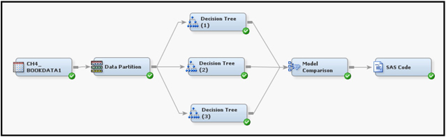

Partition the data such that 60% of the records are used for training, 30% for validation, and 10% for test.

3. Set the Nominal Criterion property to ProbChisq in Decision Tree (1) node, set it to Entropy in Decision Tree (2) node , and set it to Gini in Decision Tree (3) node. Set the Subtree Method property to Assessment and the Assessment Measure property to Decision in all three Decision Tree nodes. Use the Decision Weights shown in Display 4.1.

4. Run the three Decision Tree nodes and then the Model Comparison node.

5. Open the Results window of the Model Comparison node and compare the Cumulative % Captured Response of the three models.

6. Run the SAS Code node. Open the Code Editor window and type the following code: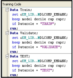

7. Type in additional SAS lines needed to print the three data sets Train, Validate, and Test. Run the code and examine the results.

8. Which decision tree is better in terms of the Cumulative % Captured Response?

Exercise 2

An auto insurance company has developed a decision tree model in order to classify the prospective customers as likely responders and non-responders. The target variable is RESP.

1. The decision tree assigns all customers who have income less than $25,000 and Age greater than or equal to 35 years to the Leaf Node 1. The decision tree also calculated the posterior probabilities as ${\hat{P}}_{1}$ ${\hat{P}}_{1}$ and ${\hat{P}}_{0}$ ${\hat{P}}_{0}$ . These posterior probabilities indicate that the probability that a customer who is assigned to the Leaf Node 1 will respond to a solicitation to apply for auto insurance is ${\hat{P}}_{1} = 0.02$ ${\hat{P}}_{1} = 0.02$ and the probability that the customer will not respond is ${\hat{P}}_{0} = 0.98$ ${\hat{P}}_{0} = 0.98$ .

2. Given the posterior probabilities given in Step 1 and using the profit matrix shown in Display 4.8, classify the customers who belong to Leaf Node 1 as Responders or Non-responders (Hint: Compare the expected profits under Decision 1 and Decision 2, where Decision 1 means labeling the customers in Leaf Node1 as responders and Decision 2 means labeling them as non-responders.)

3. After applying the decision tree to the test data set, it is found that 200 customers in the Test data set ended up in Leaf Node 1. Of these 200 customers, 6 were found to be actual responders and 194 customers were non-responders.

4. Suppose you apply the decision tree model and score a Prospect data set. If a customer from the scored data set is randomly selected and is assigned to Leaf Node 1 by the Decision Tree model, then what is the predicted probability that the customer will respond to an invitation to apply for auto insurance?

5. Given the decision you arrived at in Step 2, would you send an invitation to the customer selected in Step 4 to apply for auto insurance? Why or why not?

Notes

1. There may be a loss when a true responder is classified as a non-responder. However, in this example, I am assuming it is zero for simplicity. This assumption can be relaxed, and all the procedures shown here would apply.

2. The decision tree shown in Figures 4.1, 4.3, and 4.4 is developed using the Decision Tree node. However, the tree diagrams shown are handcrafted for illustrating various steps of the tree development process.

3. The terms target class and target level are used synonymously.

..................Content has been hidden....................

You can't read the all page of ebook, please click here login for view all page.

Table of Contents for Chapter 4: Building Decision Tree Models to Predict Response and Risk

Create new playlist

Sign In

Sign Up

Chapter 4: Building Decision Tree Models to Predict Response and Risk

4.1 Introduction