CHAPTER 22

Greedy Seeding and Problem-Specific Operators for GAs Solution of Strip Packing Problems

C. SALTO

Universidad Nacional de La Pampa, Argentina

J. M. MOLINA and E. ALBA

Universidad de Málaga, Spain

22.1 INTRODUCTION

The two-dimensional strip packing problem (2SPP) is present in many real-world applications in the glass, paper, textile, and other industries, with some variations on its basic formulation. Typically, the 2SPP consists of a set of M rectangular pieces, each defined by a width w_i and a height h_i (i = 1, …, M), which have to be packed in a larger rectangle, the strip, with a fixed width W and unlimited length. The objective is to find a layout of all the pieces in the strip that minimizes the required strip length, taking into account that the pieces have to be packed with their sides parallel to the sides of the strip, without overlapping. This problem is NP-hard [11].

In the present study some additional constrains are imposed: pieces must not be rotated and they have to be packed into three-stage level packing patterns. In these patterns, pieces are packed by horizontal levels (parallel to the bottom of the strip). Inside each level, pieces are packed bottom-left-justified, and when there is enough room in the level, pieces with the same width are stacked one above the other. Three-stage level patterns are used in many real applications in the glass, wood, and metal industries, which is the reason for incorporating this restriction in the problem formulation. We have used evolutionary algorithms (EAs) [4,15], in particular genetic algorithms (GAs), to find a pattern of minimum length. GAs deal with a population of tentative solutions, and each one encodes a problem solution on which genetic operators are applied in an iterative manner to compute new higher-quality solutions progressively.

In this chapter a hybrid approach is used to solve the 2SPP: A GA is used to determine the order in which the pieces are to be packed, and a placement routine determines the layout of the pieces, satisfying the three-stage level packing constraint. Taking this GA as our basic algorithm, we investigate the advantages of using genetic operators incorporating problem-specific knowledge such as information about the layout of the pieces against other classical genetic operators. To reduce the trim loss in each level, an additional final operation, called an adjustment operator, is always applied to each offspring generated. Here we also investigate the advantages of seeding the initial population with a set of greedy rules, including information related to the problem (e.g., piece width, piece area), resulting in a more specialized initial population. The main goal of this chapter is to find an improved GA to solve larger problems and to quantify the effects of including problem-specific operators and seeding into algorithms, looking for the best trade-off between exploration and exploitation in the search process.

The chapter is organized as follows. In Section 22.2 we review approaches developed to solve two-dimensional packing problems. The components of the GA are described in Section 22.3. In Section 22.4 we present a detailed description of the new operators derived. Section 22.5 covers the greedy generation of the initial population. In Section 22.6 we explain the parameter settings of the algorithms used in the experimentation. In Section 22.7 we report on algorithm performance, and in Section 22.8 we give some conclusions and analyze future lines of research.

22.2 BACKGROUND

Heuristic methods are commonly applied to solve the 2SPP. In the case of level packing, three strategies [12] have been derived from popular algorithms for the one-dimensional case. In each case the pieces are initially sorted by decreasing height and packed by levels following the sequence obtained. Let i denote the current piece and l the last level created:

1. Next-fit decreasing height (NFDH) strategy. Piece i is packed left-justified on level l, if it fits. Otherwise, a new level (l = l + 1) is created and i is placed left-justified into it.
2. First-fit decreasing height (FFDH) strategy. Piece i is packed left-justified on the first level where it fits, if any. If no level can accommodate i, a new level is initialized as in NFDH.
3. Best-fit decreasing height (BFDH) strategy. Piece i is packed left-justified on that level, among those where it fits, for which the unused horizontal space is minimal. If no level can accommodate i, a new level is initialized.

The main difference between these heuristics lies in the way that a level to place the piece in is selected. NFDH uses only the current level, and the levels are considered in a greedy way. Meanwhile, either FFDH or BFDH analyzes all levels built to accommodate the new piece. Modified versions of FFDH and BFDH are incorporated into the mechanism of a special genetic operator in order to improve the piece distribution, and a modified version of NFDH is used to build the packing pattern corresponding to a possible solution to the three-stage 2SPP, like the one used in refs. 18 and 21.

Exact approaches are also used [7,14]. Regarding the existing surveys of metaheuristics in the literature, Hopper and Turton [10,11] review the approaches developed to solve two-dimensional packing problems using GAs, simulated annealing, tabu search, and artificial neural networks. They conclude that EAs are the most widely investigated metaheuristics in the area of cutting and packing. In their survey, Lodi et al. [13] consider several methods for the 2SPP and discuss mathematical models. Specifically, the case where items have to be packed into rows forming levels is discussed in detail.

Few authors restrict themselves to problems involving guillotine packing [5,16] and n-stage level packing [18,19,21,23], but Puchinger and Raidl [18,19] deal in particular with the bin packing problem, where the objective is to minimize the number of bins needed (raw material with fixed dimensions) to pack all the pieces, an objective that is different from, but related to, the one considered in the present work.

22.3 HYBRID GA FOR THE 2SPP

In this section we present a steady-state GA for solving the 2SPP. This algorithm creates an initial population of μ solutions in a random (uniform) way and then evaluates these solutions. The evaluation uses a layout algorithm to arrange the pieces in the strip to construct a feasible packing pattern. After that, the population goes into a cycle in which it undertakes evolution. This cycle involves the selection of two parents by binary tournament and the application of some genetic operators to create a new solution. The newly generated individual replaces the worst one in the population only if it is fitter. The stopping criterion for the cycle is to reach a maximum number of evaluations. The best solution is identified as the best individual ever found that minimizes the strip length required.

A chromosome is a permutation π = (π₁, π₂, …, π_M) of M natural numbers (piece identifiers) that defines the input for the layout algorithm, which is a modified version of the NFDH strategy. This heuristic—in the following referred to as modified next-fit (MNF)—gets a sequence of pieces as its input and constructs the packing pattern by placing pieces into stacks (neighbor pieces with the same width are stacked one above the other) and then stacking into levels (parallel to the bottom of the strip) bottom-left-justified in a greedy way (i.e., once a new stack or a new level is begun, previous stacks or levels are never reconsidered). See Figure 22.1 for an illustrative example. A more in-depth explanation of the MNF procedure has been given by Salto et al. [23].

Figure 22.1 Packing pattern for the permutation (2 4 1 5 6 3 8 7).

The fitness of a solution π is defined as the strip length needed to build the corresponding layout, but an important consideration is that two packing patterns could have the same length—so their fitness will be equal—although from the point of view of reusing the trim loss, one of them can actually be better because the trim loss in the last level (which still connects with the remainder of the strip) is greater than the one present in the last level in the other layout. Therefore, we have used the following more accurate fitness function:

where strip.length is the length of the packing pattern corresponding to the permutation π, and l.waste is the area of reusable trim loss in the last level l.

22.4 GENETIC OPERATORS FOR SOLVING THE 2SPP

In this section we describe the recombination and mutation operators used in our algorithms. Moreover, a new operator, adjustment, is introduced.

22.4.1 Recombination Operators

We have studied five recombination operators. The first four operators have been proposed in the past for permutation representations. Three operators focus on combining the order or adjacency information from the two parents, taking into account the position and order of the pieces: partial-mapped crossover (PMX) [8], order crossover (OX) [6], and cycle crossover (CX) [17]. The fourth, edge recombination (EX) [25], focuses on the links between pieces (edges), preserving the linkage of a piece with other pieces.

The fifth operator, called best inherited level recombination (BILX), is a new one (introduced in ref. 23 as BIL) tailored for this problem. This operator transmits the best levels (groups of pieces that define a level in the layout) of one parent to the offspring. In this way, the inherited levels could be kept or could even capture some piece from their neighboring levels, depending on how compact the levels are. The BILX operator works as follows. Let nl be the number of levels in one parent, parent₁. In a first step the waste values of all nl levels of parent₁ are calculated. After that, a probability of selection, inversely proportional to its waste value, is assigned to each level and a number (nl/2) of levels are selected from parent₁. The pieces π_i belonging to the levels selected are placed in the first positions of the offspring, and then the remaining positions are filled with the pieces that do not belong to those levels, in the order in which they appear in the other parent, parent₂.

Actually, the BILX operator differs from the operator proposed by Puchinger and Raidl [18] in that our operator transmits the best levels of one parent and the remaining pieces are taken from the other parent, whereas Puchinger and Raidl recombination-pack all the levels from the two parents, sorted according to decreasing values, and repair is usually necessary to guarantee feasibility (i.e., to eliminate piece duplicates and to consider branching constraints), thus becoming a more complex and expensive mechanism.

22.4.2 Mutation Operators

We have tested four mutation operators, described below. These operators were introduced in a preliminary work [23].

The piece exchange (PE) operator randomly selects two pieces in a chromosome and exchanges their positions. Stripe exchange (SE) selects two levels of the packing pattern at random and exchanges (swaps) these levels in the chromosome. In the best and worst stripe exchange (BW_SE) mutation, the best level (the one with the lowest trim loss) is relocated at the beginning of the chromosome, while the worst level is moved to the end. These movements can help the best level to capture pieces from the following level and the worst level to give pieces to the previous level, improving the fitness of the pattern. Finally, the last level rearrange (LLR) mutation takes the first piece π_i of the last level and analyzes all levels in the pattern—following the MNF heuristic—trying to find a place for that piece. If this search is not successful, piece π_i is not moved at all. This process is repeated for all the pieces belonging to the last level. During this process, the piece positions inside the chromosome are rearranged consistently.

22.4.3 Adjustment Operators

Finally, we proceed to describe a new operator, which was introduced in a preliminary work [23] as an adjustment operator, the function of which is to improve the solution obtained after recombination and mutation. There are two versions of this operator: one (MFF_Adj) consists of the application of a modified version of the FFDH heuristic, and the other (MBF_Adj) consists of the application of a modified version of the BFDH heuristic.

MFF_Adj works as follows. It considers the pieces in the order given by the permutation π. The piece π_i is packed into the first level it fits, in an existing stack or in a new one. If no spaces were found, a new stack containing π_i is created and packed into a new level in the remaining length of the strip. The process is repeated until no pieces remain in π.

MBF_Adj proceeds in a similar way, but with the difference that a piece π_i is packed into the level (among those that can accommodate it) with less trim loss, on an existing stack or on a new one. If no place is found to accommodate the piece, a new stack is created containing π_i and packed into a new level. These steps are repeated until no piece remains in the permutation π, and finally, the resulting layout yields a suitable reorganization of the chromosome.

22.5 INITIAL SEEDING

The performance of a GA is often related to the quality of its initial population. This quality consists of two important measures: the average fitness of the individuals and the diversity in the population. By having an initial population with better fitness values, better final individuals can be found faster [1,2,20]. Besides, high diversity in the population inhibits early convergence to a locally optimal solution. There are many ways to arrange this initial diversity. The idea in this work is to start with a seeded population created by following some building rules, hopefully allowing us to reach good solutions in the early stages of the search. These rules include some knowledge of the problem (e.g., piece size) and incorporate ideas from the BFDH and FFDH heuristics [12]. Individuals are generated in two steps. In the first step, chromosomes are sampled randomly from the search space with a uniform distribution. After that, each of them is modified by one rule, randomly selected, with the aim of improving the piece location inside the corresponding packing pattern.

The rules for the initial seeding are listed in Table 22.1. These rules are proposed with the aim of producing individuals with improved fitness values and for introducing diversity into the initial population. Hence, sorting the pieces by their width will hopefully increase the probability of stacking pieces and produce denser levels. On the other hand, sorting by height will generate levels with less wasted space above the pieces, especially when the heights of the pieces are very similar. Rules 11 and 12 relocate the pieces with the goal of reducing the trim loss inside a level. Finally, rules 7 to 10 have been introduced to increase the initial diversity. As we will see, these rules are useful not only for initial seeding; several can be used as a simple greedy algorithm for a local search to help during the optimization process. The MBF_Adj operator is an example based on rule 11, and MFF_Adj operator is an example based on rule 12.

TABLE 22.1 Rules to Generate the Initial Population

Rule	Description
1	Sorts pieces by decreasing width.
2	Sorts pieces by increasing width.
3	Sorts pieces by decreasing height.
4	Sorts pieces by increasing height.
5	Sorts pieces by decreasing area.
6	Sorts pieces by increasing area.
7	Sorts pieces by alternating between decreasing width and height.
8	Sorts pieces by alternating between decreasing width and increasing height.
9	Sorts pieces by alternating between increasing width and height.
10	Sorts pieces by alternating between increasing width and decreasing height.
11	The pieces are reorganized following a modified BFDH heuristic.
12	The pieces are reorganized following a modified FFDH heuristic.

22.6 IMPLEMENTATION OF THE ALGORITHMS

Next we comment on the actual implementation of the algorithms to ensure that this work is replicable in the future. This work is a continuation of previous work [22,23], extended here by including all possible combinations of recombination (PMX, OX, CX, EX, and BILX), mutation (PE, SE, BW_SE, and LLR), and adjustment operators (MFF_Adj and MBF_Adj). Also, these GAs have been studied using different methods of seeding the initial population. All these algorithms have been compared in terms of the quality of their results. In addition, analysis of the algorithm performance was addressed in order to learn the relationship between fitness values and diversity.

The population size was set at 512 individuals. By default, the initial population is generated randomly. The maximum number of iterations was fixed at 2¹⁶. The recombination operators were applied with a probability of 0.8, and the mutation probability was set at 0.1. The adjustment operator was applied to all newly generated solutions. These parameters (e.g., population size, stop criterium, probabilities) were chosen after an examination of some values used previously with success (see ref. 21).

The algorithms were implemented inside MALLBA [3], a C++ software library fostering rapid prototyping of hybrid and parallel algorithms. The platform was an Intel Pentium-4 at 2.4 GHz and 1 Gbyte RAM, linked by fast Ethernet, under SuSE Linux with -GHz, 2.4, 4-Gbyte kernel version.

We have considered five randomly generated problem instances with M equal to 100, 150, 200, 250, and 300 pieces and a known global optimum equal to 200 (the minimum length of the strip). These instances belong to the subtype of level packing patterns, but the optimum value does not correspond to a three-stage guillotine pattern. They were obtained by an implementation of a data set generator, following the ideas proposed by Wang and Valenznela [24]. The length-to-width ratio of all M rectangles is set in the range 1/3 ≤ l/w ≤ 3. These instances are available to the public at http://mdk.ing.unlpam.edu.ar/~lisi/2spp.htm.

22.7 EXPERIMENTAL ANALYSIS

In this section we analyze the results obtained by the different variants of the proposed GA acting on the problem instances selected.

For each algorithm variant we have performed 30 independent runs per instance using the parameter values described in Section 22.6. To obtain meaningful conclusions, we have performed an analysis of variance of the results. When the results followed a normal distribution, we used a t-test for the two-group case and an ANOVA test to compare differences among three or more groups (multiple comparison test). We have considered a level of significance of α = 0.05 to indicate a 95% confidence level in the results. When the results did not follow a normal distribution, we used the nonparametric Kruskal–Wallis test (multiple comparison test) to distinguish meaningful differences among the means of the results for each algorithm.

Also, the evaluation considers two important measures for any search process: the capacity for generating new promising solutions and the pace rate of the progress in the surroundings of the best-found solution (fine tuning or intensification). For a meaningful analysis, we have considered the average fitness values and the entropy measure (as proposed in ref. 9), which is computed as follows:

where n_ij represents the number of times that a piece i is set into a position j in a population of size μ. This function takes values in [0 ··· 1], and a value of 0 indicates that all the individuals in the population are identical.

The figures in Tables 22.2 to 22.6 below stand for the best fitness value obtained (column best) and the average objective values of the best feasible solutions found, along with their standard deviations (column avg±σ). The minimum best values are printed in bold. Moreover, Tables 22.4 and 22.6 include the average number of evaluations needed to reach the best value (column eval_b), which represents the numerical effort. Table 22.3 also shows the mean times (in seconds) spent in the search for the best solution (column T_b) and in the full search (column T_t).

TABLE 22.2 Experimental Results for the GA with All Recombination and Mutation Operators

TABLE 22.3 Experimental Results for the GA with All Recombination and Mutation Operators

TABLE 22.4 Experimental Results for the GA with and Without the Adjustment Operators

TABLE 22.5 Experimental Results for the GA Using Different Seeding Methods

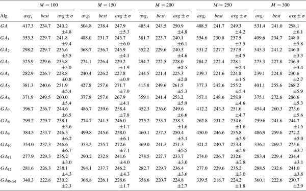
TABLE 22.6 Experimental Results for the GA with Seeding and Adjustment

22.7.1 Experimental Results with Recombination and Mutation Operators

Let us begin with the results of the computational experiments listed in Table 22.2. These results show clearly that the GA using the BILX operator outperforms GAs using any other recombination, in terms of solution quality, for all instances. In all runs, the best values reached by applying the BILX operator have a low cost and are more robust than the best values obtained with the rest of the recombination operators (see the avg±σ column), and the differences are more evident as the instance dimension increases. Using the test of multiple comparison, we have verified that the differences among the results are statistically significant.

The BILX's outperformance is due to the fact that in some way, BILX exploits the idea behind building blocks, in this case defined as a level (i.e., a group of pieces) and tends to conserve good levels in the offspring produced during recombination. As a result, BILX can discover and favor compact versions of useful building blocks.

Regarding the average number of evaluations to reach the best value (see the eval_b column in Table 22.3), BILX presents significant differences in means when compared with OX, the nearest successor regarding best values, but it does not present significant differences in means compared with EX and CX. To confirm these results, we used the test of multiple comparisons. The resulting ranking was as follows: BILX, CX, EX, PMX, and OX, from more efficient to less efficient operators.

On the other hand, the fastest approach in the search is that applying CX (see Table 22.3), due to its simplistic mechanism to generate offspring. The slowest is the GA using BILX, due to the search the best levels to transmit and to the search for pieces that do not belong to the levels transmitted. Using the test of multiple comparisons, we verified that PMX and OX have very similar average execution times, whereas the differences among the other recombination operators are significant. The ranking was CX, OX/PMX, EX, and BILX, from faster to slower operators. Although BILX exhibits the highest runtime, it is important to note that BILX is one of the fastest algorithms to find the best solution. In addition, it finds the best packing patterns; therefore, BILX has a good trade-off between time and quality of results. In conclusion, BILX is the most suitable recombination of those studied.

We turn next to analyzing the results obtained for the various mutation operators with the GA using BILX (see the BILX columns of Tables 22.2 and 22.3). On average, SE has some advantages regarding the best values. Here again we can infer that the use of levels as building blocks improves the results. The test of multiple comparisons of means shows that these differences are significant for all instances. Both BW_SE and LLR need a similar number of evaluations to reach their best values, but those values are half of the number of evaluations that SE needs and nearly a third of the number that PE needs. Despite this fast convergence, BW_SE and LLR performed poorly in solution qualities. The reason could be that those mutations make no alterations to the layout once a “good” solution is reached, whereas SE and PE always modify the layout, due to their random choices. Using the test of multiple comparisons of means, we verified that BW_SE and LLR use a similar average number of evaluations to reach the best value, while the differences between the other two mutation operators are significant. The ranking is BW_SE/LLR, SE, and PE.

With respect to the time spent in the search, we can observe that the SE and BW_SE operators do not have significantly different means, owing to the fact that their procedures differ basically in the level selection step. On the other hand, LLR is the slowest for all instances because of the search on all levels, trying to find a place for each piece belonging to the last level. As expected, PE is the fastest operator, due to its simplistic procedure. All these observations were corroborated statistically.

To analyze the trade-off between exploration and exploitation, the behavior of the various mutation operators is illustrated (for M = 200, but similar results are obtained with the rest of the instances) in Figures 22.2 and 22.3, which present the evolution of the population entropy and the average population fitness, respectively (y-axis) with respect to the number of evaluations (x-axis). From these figures we can see that genotypic entropy is higher for the SE operator with respect to the others, while average population fitness is always lower for the SE. Therefore, the best trade-off between exploration and exploitation is obtained by SE.

Figure 22.2 Population entropy for BILX and each mutation operator (M = 200).

Figure 22.3 Average fitness for BILX and each mutation operator (M = 200).

To summarize this subsection, we can conclude that the combination of BILX and SE is the best one regarding good-quality results together with a low number of evaluations to reach their best values and also with a reasonable execution time.

22.7.2 Experimental Results with Adjustment Operators

To justify the use of adjustment operators, we present in this section the results obtained by three GAs using the BILX and SE operators (see Table 22.4): one without adjustment, and the others adding an adjustment operator (MFF_Adj or MBF_Adj).

We notice that the GA variants that use some of the adjustment operators significantly outperformed the plain GA in solution quality (corroborated statistically). The reason for this is the improvement obtained in the pieces layout after the application of these operators (which rearrange the pieces to reduce the trim loss inside each level). Nevertheless, it can be observed that the average best solution quality, in general, does not differ very much between the algorithms applying an adjustment (the average best values in the last row are quite similar), whereas the differences are significant in a t-test (p-values are lower than 0.05).

Figure 22.4 shows that the two algorithms using adjustments have a similar entropy decrease until evaluation 17,000; then GA+MFF_Adj maintains higher entropy values than those of GA+MBF_Adj. An interesting point is how the incorporation of adjustment operators allows us to maintain the genotypic diversity at quite high levels throughout the search process. From Figure 22.5 we observe that the curves of GAs using adjustment operators are close; the plain GA shows the worst performance. In conclusion, GA+MFF_Adj seems to provide the best trade-off between exploration and exploitation.

Figure 22.4 Population entropy for all algorithms (M = 200).

Figure 22.5 Average population fitness for all algorithms (M = 200).

22.7.3 Studying the Effects of Seeding the Population

Up to this point we have studied GAs that start with a population of randomly sampled packing patterns. Next we analyze the results obtained when the population is initialized using problem-aware rules (see Section 22.5). We have studied GAs using the BILX and SE operators (because of the good results shown in the previous analysis) combined with three different methods of seeding the initial population: (1) by means of a random generation (GA), (2) by applying one rule from the Table 22.1 (GA_i where i stands for a rule number), and (3) by applying a rule from Table 22.1 but a randomly selected one for each individual in the population (GA_Rseed). The random generation is another rule applicable in this case.

Table 22.5 shows results obtained for the various methods of generating the initial population for all instances. In this table we include information about the average objective value of the initial population (column avg_i). Results indicate that any seeded GA starts the search process from better fitness values than the GA with randomly generated initial populations. Best initial populations, on average, are obtained using GA₄, but have poor genetic diversity (see the mean entropy values for the initial population in Figure 22.6). Rule 4 arranges the pieces by their height, so the pieces in each level have similar heights and the free space inside a level tends to be small. On the other hand, poor performance is obtained with both GA₇ and GA₉, which have the worst initial population means and also poor genetic diversity. Most of the seeded GAs present poor initial genetic diversity (below 0.5), except GA₁₂, GA₁₁, and GA_Rseed, with an initial diversity (near 1) close to that of one of the nonseeded GA_s. GA₁₂ and GA₁₁ apply modified FFDH and BFDH heuristics (respectively) to a randomly generated solution, and these heuristics do not take piece dimensions into account; hence, the original piece positions inside the chromosome suffer few modifications. On the other hand, GA_Rseed combines all the previous considerations with random generation of the piece positions, so high genetic diversity was expected (entropy value near 0.8), and the average objective value of its initial population is in the middle of the rule ranking.

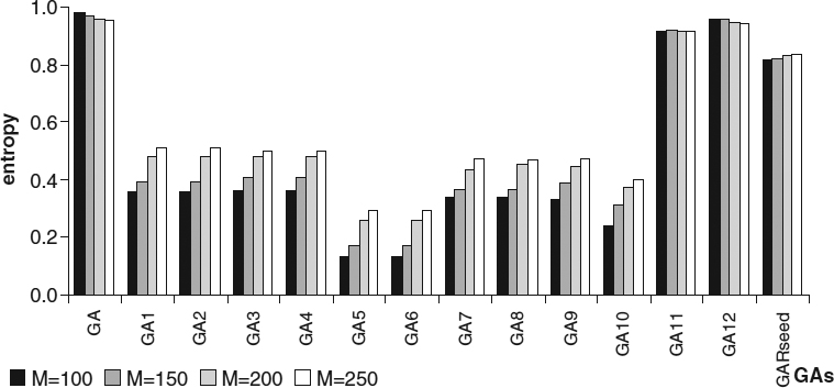
Figure 22.6 Average entropy of the initial population.

Figure 22.7 Mean number of evaluations to reach the best value for each instance.

As supposed, the GA_Rseed reduces the number of evaluations required to find good solutions (see Figure 22.7). To confirm these observations, we used the t-test, which indicates that the difference between GA_Rseed and GA is significant (p-values near 0). A neat conclusion of this study is that GA_Rseed significantly outperforms GA with a traditional initialization in all the metrics (the p-value is close to 0). This suggests that the efficiency of a GA could be improved simply by increasing the quality of the initial population.

Due to the good results obtained by the GA with the application of adjustment operators, we now compare the performance of GA_Rseed with that of two other algorithms: GA_RseedFF and GA_RseedBF, which include in their search mechanism the MFF_Adj and MBF_Adj operators, respectively.

Table 22.6 shows the results for the three approaches. For every instance, the algorithm that finds the fittest individuals is always an algorithm using an adjustment operator. Here again, there are statistical differences among the results of each group (GA_Rseed vs. GA_Rseed applying some adjustment operator), but there are no differences inside each group. Looking at the average objective values of the best solutions found, GA_RseedFF produces best values and also small deviations. In terms of the average number of evaluations, Table 22.6 (column eval_b) shows that in general, the GA_RseedFF performs faster than the other algorithms.

Finally, comparing the best values reached by the algorithms using adjustment operators with those without those operators, we observe that the results of GA_RseedFF are of poorer quality than those obtained by a nonseeded GA applying an MFF_Adj operator (the differences are significant in a t-test, with p-values very close to 0), except for instances with M = 200 and M = 300. This suggests that the operators are effective in the search process when they are applied to populations with high genotypic diversity, as shown by the plain GA (i.e., the operator has more chances to rearrange pieces in the layout). On the other hand, the means of GA_RseedFF and GA + MFF_Adj do not present significant differences in a t-test.

Both GA_Rseed using adjustment operators have a similar decrease in the average population fitness and maintain a higher entropy than does GA_Rseed (see Figures 22.4 and 22.5), but the first algorithms were able to find the best final solutions in a resulting faster convergence. In fact, we can see that the seeded initial populations present a high entropy value (near 0.85; i.e., high diversity), but GA_Rseed using adjustment operators produces fitter individuals very quickly (close to evaluation, 2000).

22.8 CONCLUSIONS

In this chapter we have analyzed the behavior of improved GAs for solving a constrained 2SPP. We have compared some new problem-specific operators to traditional ones and have analyzed various methods of generating the initial population. The study, validated from a statistical point of view, analyzes the capacity of the new operators and the seeding in order to generate new potentially promising individuals and the ability to maintain a diversified population.

Our results show that the use of operators incorporating specific knowledge from the problem works accurately, and in particular, the combination of BILX recombination and SE mutation obtains the best results. These operators are based on the concept of building blocks, but here a building block is a group of pieces that defines a level in the phenotype. This marks a difference from some of the traditional operators, who randomly select the set of pieces to be interchanged. For the 2SPP, the absolute positions of pieces within the chromosome do not have relative importance.

Also, the incorporation of a new adjustment operator (in two versions) in the evolutionary process makes a significant improvement in the 2SPP algorithms results, providing faster sampling of the search space in all instances studied and exhibits a satisfactory trade-off between exploration and exploitation. This operator maintains the population diversity longer than in the case of plain GAs.

In addition, we observe an improvement in the GA performance by using problem-aware seeding, regarding both efficiency (effort) and quality of the solutions found. Moreover, the random selection of greedy rules to build the initial population works properly, providing good genetic diversity of initial solutions and a faster convergence without sticking in local optima, showing that the performance of a GA is sensitive to the quality of its initial population.

Acknowledgments

This work has been partially funded by the Spanish Ministry of Science and Technology and the European FEDER under contract TIN2005-08818-C04-01 (the OPLINK project). We acknowledge the Universidad Nacional de La Pampa and the ANPCYT in Argentina, from which we received continuous support.

REFERENCES

1. R. Ahuja and J. Orlin. Developing fitter genetic algorithms. INFORMS Journal on Computing, 9(3):251–253, 1997.

2. R. Ahuja, J. Orlin, and A. Tiwari. A greedy genetic algorithm for the quadratic assignment problem. Computers and Operations Research, 27(3):917–934, 2000.

3. E. Alba, J. Luna, L. M. Moreno, C. Pablos, J. Petit, A. Rojas, F. Xhafa, F. Almeida, M. J. Blesa, J. Cabeza, C. Cotta, M. Díaz, I. Dorta, J. Gabarró, and C. León. MALLBA: A Library of Skeletons for Combinatorial Optimisation, vol. 2400 of Lecture Notes in Computer Science, Springer-Verlag, New York, 2002, pp. 927–932.

4. T. Bäck, D. Fogel, and Z. Michalewicz. Handbook of Evolutionary Computation. Oxford University Press, New York, 1997.

5. A. Bortfeldt. A genetic algorithm for the two-dimensional strip packing problem with rectangular pieces. European Journal of Operational Research, 172(3):814–837, 2006.

6. L. Davis. Handbook of Genetic Algorithms. Van Nostrand Reinhold, New York, 1991.

7. S. P. Fekete and J. Schepers. On more-dimensional packing: III. Exact algorithm. Technical Report ZPR97-290. Mathematisches Institut, Universität zu Köln, Germany, 1997.

8. D. Goldberg and R. Lingle. Alleles, loci, and the TSP. In Proceedings of the 1st International Conference on Genetic Algorithms, 1985, pp. 154–159.

9. J. J. Grefenstette. Incorporating problem specific knowledge into genetic algorithms. In L. Davis, ed., Genetic Algorithms and Simulated Annealing. Morgan Kaufmann, San Francisco, CA, 1987, pp. 42–60.

10. E. Hopper. Two-dimensional packing utilising evolutionary algorithms and other meta-heuristic methods. Ph.D. thesis, University of Wales, Cardiff, UK, 2000.

11. E. Hopper and B. Turton. A review of the application of meta-heuristic algorithms to 2D strip packing problems. Artificial Intelligence Review, 16:257–300, 2001.

12. A. Lodi, S. Martello, and M. Monaci. Recent advances on two-dimensional bin packing problems. Discrete Applied Mathematics, 123:379–396, 2002.

13. A. Lodi, S. Martello, and M. Monaci. Two-dimensional packing problems: a survey. European Journal of Operational Research, 141:241–252, 2002.

14. S. Martello, S. Monaci, and D. Vigo. An exact approach to the strip-packing problem. INFORMS Journal on Computing, 15:310–319, 2003.

15. M. Michalewicz. Genetic Algorithms + Data Structures = Evolution Programs, 3rd rev. ed. Springer-Verlag, New York, 1996.

16. C. L. Mumford-Valenzuela, J. Vick, and P. Y. Wang. Heuristics for large strip packing problems with guillotine patterns: an empirical study. In Metaheuristics: Computer Decision-Making. Kluwer Academic, Norwell, MA, 2003, pp. 501–522.

17. I. Oliver, D. Smith, and J. Holland. A study of permutation crossover operators on the traveling salesman problem. In Proceedings of the 2nd International Conference on Genetic Algorithms, 1987, pp. 224–230.

18. J. Puchinger and G. Raidl. An evolutionary algorithm for column generation in integer programming: an effective approach for two-dimensional bin packing. In X. Yao et al, ed., PPSN, vol. 3242, Springer-Verlag, New York, 2004, pp. 642–651.

19. J. Puchinger and G. R. Raidl. Models and algorithms for three-stage two-dimensional bin packing. European Journal of Operational Research, 183(3):1304–1327, 2007.

20. C. R. Reeves. A genetic algorithm for flowshop sequencing. Computers and Operations Research, 22(1):5–13, 1995.

21. C. Salto, J. M. Molina, and E. Alba. Analysis of distributed genetic algorithms for solving cutting problems. International Transactions in Operational Research, 13(5):403–423, 2006.

22. C. Salto, J. M. Molina, and E. Alba. A comparison of different recombination operators for the 2-dimensional strip packing problem. In Procedimiento Congreso Argentino de Ciencias de la Computación (CACIC'06), 2006, pp. 1126–1138.

23. C. Salto, J. M. Molina, and E. Alba. Evolutionary algorithms for the level strip packing problem. In Proceedings of the International Workshop on Nature Inspired Cooperative Strategics for Optimization, 2006, pp. 137–148.

24. P. Y. Wang and C. L. Valenzuela. Data set generation for rectangular placement problems. European Journal of Operational Research, 134:378–391, 2001.

25. D. Whitley, T. Starkweather, and D. Fuquay. Scheduling problems and traveling salesmen: the genetic edge recombination operator. In Proceedings of the 3rd International Conference on Genetic Algorithms, 1989, pp. 133–140.