CHAPTER 19

Application of Cellular Automata Algorithms to the Parallel Simulation of Laser Dynamics

J. L. GUISADO and F. JIMÉNEZ-MORALES

Universidad de Sevilla, Spain

J. M. GUERRA

Universidad Complutense de Madrid, Spain

F. FERNÁNDEZ

Universidad de Extremadura, Spain

19.1 INTRODUCTION

In this chapter we review the use of a biologically inspired heuristic technique—cellular automata (CA)—as a problem solver for one of the most paradigmatic complex systems: the laser. CAs are a class of mathematical system that can be used to model spatiotemporal phenomena, characterized by the discreteness of all of its variables: space, time, and normally state variables. An important property of CAs is their intrinsic parallel character. Therefore, they are specially well suited to be implemented very efficiently on parallel computers.

In this work we also exploit this property to carry out a parallel implementation of the CA model developed for laser dynamics. In addition, we study the performance and scalability of this parallel implementation and conclude that it is very satisfactory. In particular, we have described a CA-based algorithm which is an alternative to model the dynamics of lasers, normally modeled using differential equations. This approach can be very useful for modeling lasers in situations in which the differential equations are difficult to integrate, or even difficult to apply: lasers ruled by stiff differential equations, devices with complex boundary conditions, very small devices, and so on.

In Section 19.2 we introduce some background information about the relevant subjects that are treated. Then in Section 19.3 we present the problem to be solved by the proposed algorithm: laser dynamics. We describe the proposed algorithm in detail in Section 19.4. In Section 19.5 we review some of the laser properties that are reproduced successfully by the CA model. Next, we describe a parallel implementation of the CA model and analyze its performance and scalability when executed on a small computer cluster. Finally, some conclusions and prospects for future work are noted in Section 19.7.

19.2 BACKGROUND

The concept of stimulated emision was raised by Albert Einstein in his 1917 paper “Zur Quantenmechanik der Strahlung” [1]. Use of this idea has permitted us to amplify radiation by propagation across a medium in which the population of an upper energy state is larger than the population of a low-energy state (population inversion). The first experimental device working as a microwave amplifier was reported in 1955 [2]. The extension of this concept to the optical domain was achieved by Maiman in an inverted ruby rod optically pumped by a flashlamp in 1960 [3].

Maiman called this phenomenon the laser (light amplification by stimulated emission of radiation) effect. A typical laser device needs a population inversion mechanism to enhance the upper-state population to be larger than that remaining in a lower-energy state. This mechanism is usually known as the pumping system. To enhance the effective amplification, the inverted medium is usually placed inside a Fabry–Perot resonator that provides feedback, making the amplified light bounce between the mirrors. In this form the laser behaves as a regenerative light oscillator, and transient, periodic, or chaotic oscillatory processes arise in it. The amplification gain is spread homogeneously or inhomogeneously over an interval of frequencies, frequently covering several resonator mode frequencies. In some cases the light in many of the covered resonator modes becomes amplified, frequently coupled in phase, causing a large variety of complex dynamic phenomena to take place. In the case of large-aperture lasers, a large number of transverse mode geometries may be developed by the system, and the dynamic behavior has a spatiotemporal character. In many cases the spatiotemporal dynamics of these lasers has been observed to be complex [4], but in homogeneously broadened gain, lasers may be fairly well reproduced by simple theoretical models [4]. In these models a single frequency field in resonant interaction with the populations of a couple of states in the medium is assumed. In this simplified model, field and matter obey the Maxwell–Bloch equations [5]. These equations couple the electromagnetic field with matter polarization and population inversion. The dynamics is influenced by the relaxation constants of field, atomic polarization, and population inversion, the lowest of the tree damping constants becoming dominant. Frequently, the polarization damping constant is the largest and the polarization becomes a slave of field and population inversion. By eliminating the polarization from the equations and under an assumption of homogeneous field spatial distribution, a couple of rate equations may describe some simple laser dynamics.

The Maxwell–Bloch equations are 2 + 1 partial differential equations with damping constants sometimes several orders of magnitude different. Thus, integration of this system is sometimes a very rigid problem. For this reason, an alternative approach to modelization would be welcome. Cellular automata models may play an important role in this context, taking into account its intrinsic parallelization in computing. To test the feasibility of this approach, we have started from simulation of the simplest rate equations.

In this work we first describe a CA algorithm to model a simple laser device, and after reviewing some of the laser dynamics phenomena that are reproduced by the CA model, we develop a parallel implementation of the model to be executed on parallel computers. The very nature of cellular automata is strongly connected with parallel systems: The reason is the way a CA works, by simultaneous updating of a cell's states along the entire automaton. No sequential process should therefore be employed for that task, but instead, a parallel computation of new states for all the cells. Nevertheless, despite the intrinsic parallel nature of the model, researchers have usually applied sequential processes that simulate the parallel processes. The reason is the sequential nature of the computers generally used for simulations. Although this is an easy approach to employing CA systems, they would be of no practical use for solving real-world problems because of the computational load for large sizes of two- or three-dimensional CA.

The possibilities for running CA in parallel are two: The first consists of using available parallel computers to develop parallel CA; the second requires the design of specialized hardware aimed at CA execution. Although some attempts have been described for this second alternative, such as the CAM (cellular automata machine) computer [6], we focus here on available parallel, cluster, or grid deployment of CA. In fact, general-purpose parallel computers are well suited for scalable CA models, from the point of view of speedup, programmability, and portability. Two types of architectures are of interest: both single-instruction and multiple-data (SIMD) and also multiple-instruction, multiple-data (MIMD). For the implementation of CA on these computers, two principal approaches are available: using general-purpose parallel programming languages such as HPF, HPC++, or Linda, or employing a standard high-level sequential language combined with specific libraries allowing parallel applications to run, such as MPI (message-passing interface), PVM (parallel virtual machine), or OpenMP (open multiprocessing).

During the last decade, some attempts to introduce parallelism within CA have been described. Most of them were not intended to implement directly the inherently parallel CA internal working rules, which can easily be simulated in sequential fashion, but to improve speedup of the entire process by using many processors. The first attempts to parallelize CA were carried out by Resnick with the StarLogo system [7] and by Cannataro et al. [8], although many approaches and results were described later using parallel CAs, such as CAMEL [9], Nemo [10], PECANS [11], DEVS [12], and P-CAM [13]. The topic has been reviewed by Talia [14].

19.3 LASER DYNAMICS PROBLEM

We start by modeling the simplest laser dynamics phenomena, which can be described in the most simplified but still realistic way by two coupled nonlinear rate equations [15]:

The first gives the variation in the number of laser photons n(t) with time, proportional to the laser beam intensity. The term +KN(t)n(t) represents an increase in the number of photons by stimulated emission (K is the coupling constant between the radiation and the population inversion). The term −n(t)/τ_c accounts for the decaying (or absorption) process exhibited by laser photons inside a laser cavity with a characteristic decay time τ_c. The second equation represents the temporal variation of the population inversion N(t). The term +R(t) represents the pumping of electrons with a pumping rate R to the upper laser level. The term −N(t)/τ_a introduces the decaying of electrons from the upper laser level to lower levels with a characteristic decay time τ_a. The product term −KN(t)n(t) reflects decreasing population inversion by stimulated emission. The presence of the product term KN(t)n(t) in each equation gives them a nonlinear nature. For small-amplitude fluctuations, its solutions can show relaxation oscillations in their evolution toward a steady state. For strong oscillations the two variables n(t) and N(t) are changing in a rapid and typically nonlinear way, and there does not seem to be a simple analytical solution [15, 16].

A simplified but sufficiently realistic description of the laser system represented by these equations is the four-level laser system depicted in Figure 19.1, where we have represented some of the basic physical processes that play a role. Electrons are excited from the ground level up to level E₃ by some external pumping process. Population inversion is produced between levels E₁ and E₂. The reason is that the lifetimes of energy levels E₃ and E₁ are negligible compared to the lifetime of level E₂. As a result, electrons in levels E₃ and E₁ decay very fast, but level E₂ is metastable. Stimulated emission occurs when an electron in level E₂ decays down to level E₁, stimulated by the presence of a stimulator photon with energy E = E₂ − E₁. Two processes not represented in Figure 19.1 are also very important: absorption of electrons in level E₂ (which decay to lower levels due to different processes not related to stimulated emission) and absorption of laser photons, a fraction of which disappear because they leave the laser cavity through the semireflecting mirror or are absorbed by the material.

Figure 19.1 Some of the basic physical processes in a four-level laser system, a simplified but still realistic description of many real laser systems.

19.4 ALGORITHMIC PROPOSAL

In this section we describe the algorithm that we have used to simulate laser dynamics, proposed originally by some of the present authors [16]. The algorithm is based on a two-dimensional, partially probabilistic multivariable CA that simulates a transverse section of the active medium in a laser system. The defining characteristics of the CA are described below.

19.4.1 Cellular Space

The cellular space is a two-dimensional square lattice that contains N_c = L × L cells. Periodic boundary conditions are used.

19.4.2 States of the Cells

Two variables are associated with each cell of the CA: a_ij(t) and c_ij(t). The first, a_ij(t), represents the state of the electron in cell {ij} (row i and column j) at time t: When a_ij(t) = 0, the electron is in the ground state, and when a_ij(t) = 1, the electron is in the upper laser state. Also, c_ij(t) ∈ {0,1,2, …, M} represents the number of laser photons in cell {ij} at time t. This number is bounded by an upper value M which must be chosen large enough to avoid the saturation of the system. The state variables represent “bunches” of real photons and electrons. Its values are connected to the number of photons and electrons in the real system by a normalization constant.

Figure 19.2 Moore neighborhood.

19.4.3 Neighborhood

Each cell interacts locally with a number of surrounding cells belonging to a Moore neighborhood: the cell itself (C), its four nearest neighbors located at the north (N), south (S), east (E), and west (W) positions, and the four next-nearest neighbors, located at the northeast (NE), southeast (SE), southwest (SW), and northwest (NW) positions, as shown in Figure 19.2.

19.4.4 Transition Rules

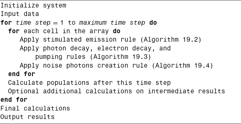
The evolution of the system is computed using the transition rules, which specify the state of each cell at time step t + 1, depending on its state and the state of the cells included in its neighborhood at time step t. Rules represent the physical processes working at the microscopic level in the laser system. The application of the transition rules is the main operation of a CA algorithm. In our case the overall structure of the CA laser model algorithm is shown in Algorithm 19.1, which corresponds to the main program. After initializing the system, the transition rules are applied to each CA cell inside a time loop. Subroutines used for computation of the transition rules are shown in Algorithms 19.2 to 19.5.

Algorithm 19.1 Pseudocode Diagram for the CA Laser Model

Our CA model uses five transition rules:

1. Stimulated emission rule (Algorithms 19.2 and 19.3). If the electronic state of a cell has a value of a_ij(t) = 1 at time t and the sum of the values of the laser photons states in the nine neighboring cells is larger than a certain threshold θ (which in our simulations has been taken to be 1), then at time t + 1 a new photon will be emitted in that cell: c_ij(t + 1) = c_ij(t) + 1, and the electron will decay to the ground level: a_ij(t + 1) = 0. All the cells of the CA must be updated in parallel. To this end, changes from this rule are computed using a temporal matrix . After the rule has been applied to all the cells of the CA, the values of c_ij are updated with the contents of .

2. Photon decay rule (Algorithm 19.4). Each photon is destroyed τ_c time steps after being created. In particular, (tlc_ijk) represents the number of time steps that will have to elapse until a particular photon located in cell {ij} (at row i and column j) is destroyed, where k distinguishes between the different photons that can occupy the same cell. When a photon is created, tlc_ijk = τ_c. After that, 1 is substracted from tlc_ijk at each time step and the photon will be destroyed when tlc_ijk = 0.

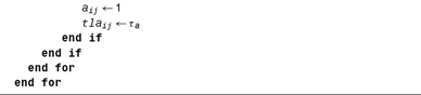
3. Electron decay rule (Algorithm 19.4; this algorithm computes three rules: photon decay, electron decay, and pumping). After an electron is excited from the ground level to the upper laser level, it will decay to the ground level again after τ_a time steps if it has not yet decayed by stimulated emission. In particular, (tla_ij) represents the number of time steps that will have to elapse until a particular electron located in cell {ij} decays to the ground level. When the electron is excited initially, tla_ij = τ_a. After that, 1 is substracted from tla_ij at each time step and the electron will decay to the ground level again when tla_ij = 0.

4. Pumping rule (Algorithm 19.4). If the electronic state of a cell {ij} has a value of a_ij(t) = 0 at time t, then at time t + 1 that state will have a value of a_ij(t + 1) = 1 with a pumping probability λ.

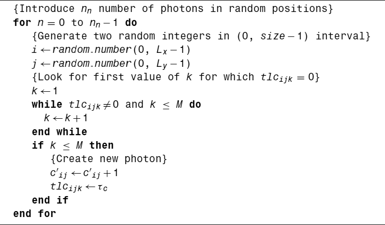
5. Noise photons creation (Algorithm 19.5). A small number of laser photons in randomly chosen positions is introduced at each time step to reproduce spontaneous emission and thermal contributions, responsible for the initial laser startup. To this end, for a small number of randomly chosen cells {ij} (< 0.01% of total), c_ij(t + 1) = c_ij(t) + 1 is applied.

19.5 EXPERIMENTAL ANALYSIS

In this section we present a review of some of the experimental results found in the simulations carried out using this model. As shown originally [16–19], the CA model of laser dynamics can reproduce different aspects of the phenomenology of laser systems. The behavior of the system depends on three parameters: the pumping probability (λ), the lifetime of photons (τ_c), and the lifetime of excited electrons (τ_a). In a simulation, an initial state is provided [a_ij(0) = 0, c_ij(0) = 0, ∀ij, except for a small fraction, 0.01%, of noise photons present] and then the system is allowed to evolve for a number of time steps. In each step we measure two macroscopic magnitudes: the total number of laser photons, n(t), and the total number of electrons in the upper laser state (population inversion), N(t):

Algorithm 19.2 Stimulated Emission Rule

Algorithm 19.3 Function to Calculate the Sum of Photons in State 1 in the Moore Neighborhood, Implementing Periodic Boundary Conditions

A characteristic feature of laser systems is that laser action happens only when the pumping probability is over a threshold value. This property is reproduced correctly by the CA model [16], and the dependence of this threshold value on the other two system parameters (lifetimes τ_a and τ_c) is found to be in good agreement with laser behavior, as shown in Figure 19.3. Depending on the values of their three characteristic parameters, lasers exhibit two main distinctive behaviors in their time evolution: a constant or an oscillatory behavior [16, 18]. As shown in Figure 19.4, the model reproduces these two types of behavior: The time evolution obtained from the simulations is similar to that exhibited by laser systems, described, for example, by Siegman [15]. A lattice size of 400 × 400 cells was used for this figure.

Algorithm 19.4 Photon Decay, Electron Decay, and Pumping Rules

Algorithm 19.5 Noise Photons Creation Rule

In addition, the CA model exhibits another type of complex behavior in which irregular oscillations with fluctuations on a wide range of time scales appear (see ref. 18), as shown in Figure 19.5. This regime could correspond to a chaotic state, as found in the dynamics of many lasers, but this is still under investigation. Also, the dependence on system parameters of the type of behavior exhibited in the time evolution of the system is in good qualitative agreement with the laser behavior [16], as shown in Figure 19.6. In this figure we show a contour plot of a magnitude called Shannon's entropy of the distribution of the number of laser photons, for a fixed value of τ_c = 10 time steps and obtained using simulations with a 200 × 200 lattice.

This magnitude is a good indicator of the presence of oscillations in the time evolution of the number of laser photons (for a precise definition and discussion, see, e.g., ref. 17). In this plot, R is the laser pumping rate and R_t is the threshold laser pumping rate, which are linearly related to the pumping probability λ and the threshold pumping probability λ_t that appear in the CA model, so that R/R_t = λ/λ_t. Points a, b, and c show the values of the parameters that correspond to Figures 19.4 and 19.5: a corresponds to constant behavior [Figure 19.4(a)], b to oscillatory behavior [Figure 19.4(b)], and c to a regime with irregular oscillations (Figure 19.5). High values of Shannon's entropy (dark zones) correspond to oscillatory behavior and low values (bright zones) to nonoscillatory response. The predictions of the standard laser rate equations are indicated by the black line: Areas of oscillatory behavior should appear above and to the right of this curve, and constant behavior should appear in the remaining areas. There is good qualitative agreement between the predictions and the results of the simulations indicated by Shannon's entropy, as the high values of this magnitude appear above and to the right of the black line, and their contour resembles the shape of this line.

Figure 19.3 Dependence of the threshold pumping probability λ_t from the CA laser model on the product of the characteristic lifetimes τ_a and τ_c (measured in time steps), plotted on a logarithmic scale. The solid line is the laser behavior predicted by the standard laser rate equations, and the dots are the results of the simulations.

19.6 PARALLEL IMPLEMENTATION OF THE ALGORITHM

Earlier we described a CA algorithm employed to simulate laser dynamics and presented some of its experimental results. It was shown that a very simple coarse-grained CA model can reproduce the laser behavior in a qualitative way. But a finer-grained CA model is needed to simulate a specific laser device quantitatively. In particular, it could reproduce more details of that specific device (such as complicated boundary conditions) and have a granularity closer to that of the real macroscopic system. Moreover, to reproduce the shape of the laser device, a three-dimensional version of the CA model is needed. For these purposes a very large lattice size is needed, and the resulting algorithm needs a prohibitively large runtime for a sequential computer. Therefore, a parallel implementation is needed. In the present section we describe a parallel implementation of the previous CA model and study its performance and scalability running on a small computer cluster. These results were introduced in refs. 19 and 20.

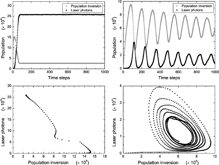
Figure 19.4 Simulation results for two different sets of values of the system parameters depicting the time evolution of the two macroscopic magnitudes, number of laser photons n(t) and population inversion N(t). They show how the model reproduces the two main characteristic behaviors exhibited by lasers. Upper: n(t) and N(t) versus time. Lower: evolution in a phase space with n(t) versus N(t). Left: Constant behavior; parameters: {λ = 0.192, τ_c = 10, τ_a = 30}. After an initial transient, the system goes to a fixed point. Right: Oscillatory behavior; parameters: {λ = 0.0125, τ_c = 10, τ_a = 180}. The system follows a spiral toward a steady-state limit point.

The CA model has been parallelized for running on parallel computers with distributed memory using the message-passing paradigm. The parallel virtual machine (PVM) implementation of this paradigm has been used because we were interested in a later study of the model using dynamic load-balancing mechanisms developed for it specifically. Parallelization has been done using the master–slave programming model, as shown in Figure 19.7. Workload has been allocated with data decomposition methodology: Identical tasks are computed with different portions of the data. A master program performs the initialization of the system, divides the CA lattice in p partitions of equal size, and sends each to a slave program that runs on a different processor. The particular tasks carried out by the master and slave programs are:

Figure 19.5 Regime with irregular oscillations for λ = 0.031, τ_c = 10, τ_a = 180. The number of laser photons and population inversion are plotted versus time after a transient of 500 time steps. Lattice size: 400 × 400 cells.

Figure 19.6 Contour plot of Shannon's entropy of the distribution of the number of laser photons obtained from the simulations with a fixed value of τ_c = 10 time steps. This plot shows that there is good qualitative agreement between dependence on system parameters of the type of behavior exhibited by the system, as obtained from the simulations, and the laser behavior, delimited by the black line.

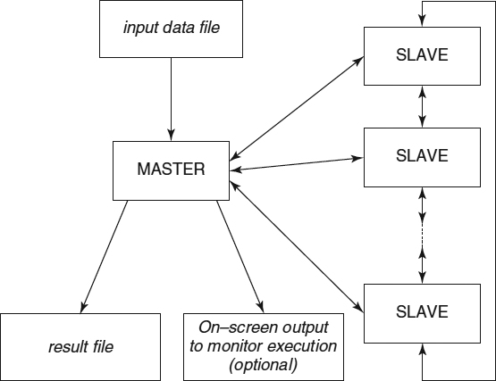
Figure 19.7 Block diagram of the parallel implementation of the CA model of laser dynamics, showing processes running on different processors (boxes in bold type represent different processors), communications between them (bold lines), and data flows.

• Master program
  1. Reading input data (system size, number of partitions, parameter values, number of time steps) and initialization
  2. Spawning slave programs
  3. Partitioning the initial data of the automaton
  4. Sending common information and initial data to each slave
  5. Collection of results from slaves at each time step
  6. Termination of slave programs
  7. Calculations performed using collected data
  8. Outputting final data to external files
  9. Timing functions to measure performance
• Slave program
  1. Reception of common information and initial data from master
  2. Time evolution computation for the assigned partition: application of CA evolution rules
  3. Exchange of state of the boundary cells with slave programs computing the neighboring partitions
  4. Computation of intermediate results and their communication to the master program

A one-dimensional domain decomposition has been used: The CA is divided vertically into parallel stripes (subdomains), and each is assigned to a different processor. Two additional columns of ghost cells have been included at the left and right sides of each subdomain. They store the state of neighboring cells, which belong to a different subdomain that will be needed to apply the transition rules to the cells of the original subdomain. For the transition rules of our CA model, the only state information needed from neighboring cells is the photon state c_ij(t), so this is the only information that must be communicated from the neighboring subdomains. Each slave program is responsible for computing the time evolution on its assigned partition.

We have measured the performance and scalability of the parallel implementation by running simulations on the cluster Abacus from the University of Extremadura, a Beowulf-type cluster composed of 10 nodes with an Intel Pentium-4 processor, six with a clock frequency of 2.7 GHz and four with 1.8 GHz, communicated by a fast Ethernet switch with 100 Mbps of bandwith. To avoid indeterminism in the results due to the heterogeneity of the cluster, for simulations with one to six nodes, slave programs have always been run on the “fast” (2.7-GHz) machines, and for simulations with seven to 10 nodes, additional “slow” (1.8-GHz) machines have been used to complete the required number of nodes. The master program has always been run on the master node of the cluster (1.8 GHz).

To measure the performance of the parallel implementation, we have run the same experiment for three different system sizes using a different number of partitions (each assigned to a slave program running on a different processor). The resulting runtime measures are plotted in Figure 19.8, showing a significant decrease in the number of processors. The only exception is the change from six to seven processors, where an increase is registered due to the assigning strategy that has been used: Only fast nodes are assigned to jobs with six or fewer processors, and for jobs with more than six processors, some slow processors have to be used.

The performance of the parallel application can be evaluated using speedup (S_p) [21], which indicates how much faster a parallel algorithm is than a corresponding sequential algorithm. It can be defined as the ratio of the runtime of the sequential version of the program running on one processor of the parallel computer (T₁) to the runtime of the parallel version running on m processors of the same computer (T_m):

Figure 19.8 Runtime of the experiments, using a logarithmic scale, for different numbers of partitions of the whole CA, each running on a different processor. Measurements for three different system sizes are shown.

In Figure 19.9 we have shown the speedup obtained for parallel implementation of our CA model [19] for three different system sizes, compared to linear speedup, represented by the line y = x, which could be defined as the ideally optimal speedup. For the smallest system size, very good performance has been obtained. For the other two system sizes, still better performance figures are obtained: in fact, superlinear speedup (speedup higher than linear). The reasons are finite memory effects on the memory hierarchy: For very large system sizes, the physical memory of one processor is not enough and swap memory must be used, thus considerably increasing the runtime for the sequential version of the program and obtaining a speedup value higher than lineal. Because of this circumstance the calculation for very large system sizes (e.g., for a detailed three-dimensional simulation) may not be affordable on a single PC (for the prohibitively large runtime needed due to the use of swap memory) but be feasible on a cluster, in which the system is partitioned so that each node needs less memory and does not have to use swap memory.

Figure 19.10 is a Gantt chart representing the various types of tasks executed for each node and the messages transferred between different nodes versus time. The activity of the master node, which executes only the master program, is represented above and the activity from the six slave nodes executing the slave program is represented below it. Two different periods can be recognized: computation periods, represented by dark gray horizontal rectangles, in which each slave node calculates the CA state for the next time step on its subdomain, and the communication periods, represented by white horizontal rectangles, in which the photon state values of the cells located in the borders of each subdomain are communicated to the slave node responsible for the neighboring subdomain, and the total number of electrons and photons in each subdomain are sent to the master node. These communications are carried out by exchanging messages, represented by the thin lines joining execution points from different nodes. Computation periods are much longer than communication periods, as can be deduced by the length of the horizontal rectangles. The average computation-to-communication ratio for the slave nodes, obtained by calculating the ratio between the average horizontal length of their dark gray and white rectangles, is on the order of 10. This indicates that the application is taking good advantage of the parallelization on the computer cluster [19].

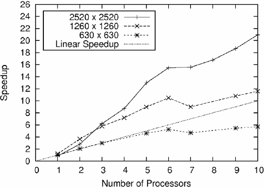
Figure 19.9 Speedup obtained for the parallel implementation with respect to the sequential program for different numbers of processors and for three different system sizes. For comparison, the ideally optimal linear speedup has been shown. Very good performance is obtained for a moderate system size (630 × 630 cells) and a superlinear speedup for larger system sizes.

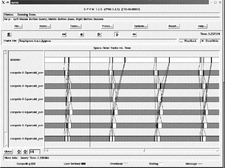
Figure 19.10 Gantt chart with the tasks executed by each cluster node and the messages passed between different nodes versus time once the calculation phase has started. It shows that the application is running with a high computation-to-communication ratio, on the order of 10, and therefore it is exploiting the parallel computational power of the machine.

Finally, it is interesting to ask if the parallel implementation of the model is scalable for clusters of this order of magnitude. Following Dongarra et al. [22], an application is said to be scalable if when the number of processors and the problem size are increased by a factor of x, the running time remains the same. To analyze this question, we have run the same experiment, increasing the system size and the number of processors by the same factor. The results are shown in Figure 19.11. In an ideal case, the running time should be the same for all cases. In our case, only a small excess (from 2 to 5%) of runtime compared to the optimal value was obtained, showing that the parallel implementation scales well on a small computer cluster [19].

Figure 19.11 Scalability of the combination parallel application–parallel computer can be analized by comparing the runtimes obtained for the same experiment when increasing the system size and the number of processors by the same factor. For an optimal ideal scalability, the same runtime (horizontal straight line) would be obtained. Here, a small excess in runtime from the optimal value (from 2 to 5%) is obtained. It shows that the parallel implementation scales well at this level of parallelization.

19.7 CONCLUSIONS

In this chapter we have reviewed the use of a cellular automata-based algorithm to simulate the time evolution of a complex system: laser dynamics. In addition, we have described how to implement this algorithm in parallel for computer cluster environments, and we have studied the performance and scalability of such an implementation on a small cluster. As a result, we can conclude that the CA algorithm described is a useful technique as an alternative to the standard description of laser dynamics for certain situations. Furthermore, it is feasible to run large fine-grained or three-dimensional simulations of specific real laser systems with the CA model using the parallel implementation on computer clusters, simulations that are not possible on a single-processor sequential computer for their large runtime and memory requirements.

Once the feasibility of running large simulations of the CA model is proved, some of the steps that can be taken to continue this research line are: developing a three-dimensional model with more realistic boundary conditions, verifying that it reproduces the behavior of specific real laser devices, and studying the feasibility of extending the present parallel model to parallel computing environments beyond cluster computing, such as grid computing.

Acknowledgments

This work was partially supported by the Spanish MEC and FEDER under contract TIN2005-08818-C04-03 (the OPLINK project).

REFERENCES

1. A. Einstein. Zur Quantenmechanik der Strahlung. Physikalische Zeitschrift, 18:121–128, 1917.

2. J. P. Gordon, H. J. Zeiger, and C. H. Townes. The maser, new type of microwave amplifier, frequency standard, and spectrometer. Physical Review, 99:1264–1274, 1955.

3. T. H. Maiman. Optical and microwave-optical experiments in ruby. Physical Review Letters, 4:564–566, 1960.

4. E. Cabrera, S. Melle, O. Calderón, and J. M. Guerra. Evolution of the correlation between orthogonal polarization patterns in broad area lasers. Physical Review Letters, 97:233902, 2006.

5. L. A. Lugiato, G. L. Oppo, J. R. Tredicce, L. M. Narducci, and M. A. Pernigo. Instabilities and spatial complexity in a laser. Journal of the Optical Society of America, 7:1019, 1990.

6. T. Toffoli and N. Margolus. Cellular Automata Machines: A New Environment for Modelling. MIT Press, Cambridge, MA, 1987.

7. M. Resnick. Turtles, Termites, and Traffic Jams. MIT Press, Cambridge, MA, 1994.

8. M. Cannataro, S. Di Gregorio, R. Rongo, W. Spataro, G. Spezzano, and D. Talia. A parallel cellular automata environment on multicomputers for computational science. Parallel Computing, 21(5):803–823, 1995.

9. G. Spezzano, D. Talia, S. Di Gregorio, R. Rongo, and W. Spataro. A parallel cellular tool for interactive modeling and simulation. IEEE Computational Science and Engineering, 3(3):33–43, 1996.

10. D. Hutchinson, L. Kattner, M. Lanthier, A. Maheshwari, D. Nussbaum, D. Roytenberg, and J. R. Sack. Parallel neighbourhood modeling: research summary. In Proceedings of the 8th Annual ACM Symposium on Parallel Algorithms and Architectures, 1996, pp. 204–207.

11. L. Carotenuto, F. Mele, M. Furnari, and R. Napolitano. PECANS: a parallel environment for cellular automata modeling. Complex Systems, 10(1):23–42, 1996.

12. B. Zeigler, Y. Moon, D. Kim, and G. Ball. The DEVS environment for high-performance modeling and simulation. IEEE Computational Science and Engineering, 4(3):61–71, 1997.

13. A. Schoneveld and J. F. de-Ronde. P-CAM: a framework for parallel complex systems simulations. Future Generation Computer Systems, 16(2):217–234, 1999.

14. D. Talia. Cellular processing tools for high-performance simulation. IEEE Computer, 33(9):44–52, 2000.

15. A. E. Siegman. Lasers. University Science Books, Mill Valley, CA, 1986.

16. J. L. Guisado, F. Jiménez-Morales, and J. M. Guerra. Cellular automaton model for the simulation of laser dynamics. Physical Review E, 67(6):066708, 2003.

17. J. L. Guisado, F. Jiménez-Morales, and J. M. Guerra. Application of Shannon's entropy to classify emergent behaviors in a simulation of laser dynamics. Mathematical and Computer Modelling, 42:847–854, 2005.

18. J. L. Guisado, F. Jiménez-Morales, and J. M. Guerra. Computational simulation of laser dynamics as a cooperative phenomenon. Physica Scripta, T118:148–152, 2005.

19. J. L. Guisado, F. Jiménez-Morales, and F. Fernández de Vega. Cellular automata and cluster computing: an application to the simulation of laser dynamics. Advances in Complex Systems, 10(1):167–190, 2007.

20. J. L. Guisado, F. Fernández de Vega, and K. Iskra. Performance analysis of a parallel discrete model for the simulation of laser dynamics. In Proceedings of the International Conference on Parallel Processing Workshops. IEEE Computer Society Press, Los Alamitos, CA, 2006, pp. 93–99.

21. I. Foster. Designing and Building Parallel Programs. Addison-Wesley, Reading, MA, 1995.

22. J. Dongarra, I. Foster, G. Fox, W. Gropp, K. Kennedy, L. Torczon, and A. White. Sourcebook of Parallel Computing. Morgan Kaufmann, San Francisco, CA, 2003.