This chapter describes the principles and formation mechanism of solitons in a lasing cavity formed in guided wave structures, especially the single-mode fibers. Mathematical equations essential for the generation and propagation in the cavity are given.

3.2 Nonlinear Schrödinger Equations

In order to appreciate the propagation of optical pulses in a nonlinear guided medium, Maxwell’s equations are employed to derive the nonlinear wave evolution equation (see also Appendix A) that describes lightwave confinement and propagation in optical waveguides including optical fibers as follows [1]:

Using the vector identity and for dielectric materials, the nonlinear wave propagation in nonlinear waveguide in the time-spatial domain in vector form can be expressed as

where is the electric field vector of the optical wave, is the vacuum permeability assuming a nonmagnetic wave-guiding medium, c is the speed of light in vacuum, , are, respectively, the linear and nonlinear parts of polarization vector, which are formed as

where χ⁽¹⁾ and χ⁽³⁾ are the first- and third-order susceptibility tensors. Thus, the linear and nonlinear coupling effects in optical waveguides can be described by Equation (3.2). In optical waveguides such as optical fibers, only the third-order nonlinearity is of special importance because it is responsible for all nonlinear effects. The second term on the right-hand side of Equation (2.3) is responsible for nonlinear processes including interaction between optical waves through the third-order susceptibility. If the nonlinear response is assumed to be instantaneous, the time dependence of χ⁽³⁾ is given by the product of three delta functions of the form δ(t − t₁) and then Equation (4.3) reduces to

where χ⁽¹⁾ and χ⁽³⁾ are the second- and fourth-rank tensors, respectively.

To simplify the analysis of Equation (3.2), the following assumptions will be made:

• Only one mode is present in the waveguide or a single-mode fiber is considered.

• The field is linearly polarized in the same direction and the polarization state remains unchanged during the propagation.

• The nonlinearity can be seen as a small perturbation because nonlinear change in the refractive index is Δn/n < 10⁻⁶ in practice.

• The variation of the carrier wave is much faster than that of the envelope of the optical pulse. On the other hand, the bandwidth of the optical pulse Δω is much smaller than the carrier frequency ω₀.

In this approximation of the slowly varying envelope, the electric field can be written in the form:

where w₀ is the carrier frequency, is the polarization unit vector, and is a slowly varying function of time, can also be expressed in a similar manner. Introducing (3.6) into (3.3) and (3.5) yields

The first term in (3.8) describes the nonlinear part of the polarization at three times the original carrier frequency, which is responsible for the third harmonic generation (THG) and requires phase matching. The second term describes the nonlinear part of the polarization at the carrier frequency and is responsible for most of important nonlinear effects relating to the nonlinear refractive index.

The linear and nonlinear parts of polarization are related to the dielectric constant as

where ε_L, ε_L are the linear and nonlinear contributions to the dielectric constant and are obtained from (3.7) and (3.8):

This dielectric constant can be used to define the refractive index n(w) and the absorption coefficient α(w) of the nonlinear medium as follows:

Both n(w) and α(w) relate to the linear and nonlinear parts of ε(w) by introducing

where the linear index n₀ and the absorption coefficient α₀ are related to the real and imaginary parts of while the nonlinear index n₂ and the two-photon absorption coefficient α₂ are related to the real and imaginary parts of ε_NL by

For some optical waveguides such as optical fibers, the coefficient α₂ is negligible and the nonlinear refractive index is responsible for the nonlinear response of the propagation medium.

3.2.1 Nonlinear Schrödinger Equation

The nonlinear Schrödinger equation (NSE) plays an important role in the description of nonlinear effects in optical pulse propagation. It can be derived from the wave Equation (2.3) after some algebra by using the method of separating variables (see Appendix A):

where A(z,t) is the slowly varying complex envelope propagating along z in the propagation medium, the effect of propagation constant β around the optical carrier w₀ is the Taylor-series expanded, R(t) is the nonlinear response function, and is the nonlinear coefficient. We note here that the optical frequency term has been removed and only the amplitude of the modulated lightwaves is involved whose complex term would contain the phase of the lightwave carrier. Thus, we will see later that the software package developed for the propagation of the lightwave envelope involves the complex amplitude. This gives advantages as the optical frequency is very high and it is impossible to sample the wave at this frequency in current computing systems.

In most cases in optical communications application, the optical pulses with the width larger than 100 fs are employed, Equation (14.3) can be further simplified as

where a frame of reference moving with the pulse at the group velocity v_g is used by making the transformation, and the propagation constant is expanded up to the third-order term that includes the group velocity dispersion (β₂) and the third-order dispersion (β₃). In (3.15), the first moment of the nonlinear response function is defined as

which is responsible for the Raman scattering effect, and the second term in the right side of (3.15) is responsible for the self-steepening effect. However, if the width of optical pulses is of the order of picoseconds, the high-order effects such as self-steepening and Raman scattering can be ignored. Hence, Equation (15.3) becomes

This equation can describe the most important linear and nonlinear propagation effects of optical pulse in optical fibers.

If we further simplify Equation (17.3) by setting the attenuation factor and the third-order dispersion coefficient to zero, then the traditional NLS can be obtained as

Equation (3.18) is a well-known equation in nonlinear fiber optics which is employed to explain propagation of optical solitary waves in nonlinear dispersive medium.

3.2.2 Ginzburg–Landau Equation: A Modified Nonlinear Schrödinger Equation

Although the NSEs described above can be used to explain most nonlinear effects including higher-order effects, they only describe the pulse propagation in passive nonlinear media without gain. In a propagation medium with gain as fiber amplifiers, the gain effect is required to be included in the NLS equation. The general equation that governs the pulse propagation in active fibers is given by ignoring other effects for simplification as follows:

where g(w) is the gain coefficient of the active fiber. For an approximation of a homogeneously broadened system, the gain spectral shape takes a Lorentzian profile [2]:

where g₀ is the maximum small signal gain, w_g is the atomic transition frequency, and Δω_g is the gain bandwidth that relates to the dipole relaxation time. The gain spectrum can be approximated by the Taylor expansion in the neighborhood of ω_g given by

Thus, by substituting (3.21) into (3.19), and taking the inverse Fourier transform with an assumption of the carrier frequency ω₀ close to ω_g, the propagation equation with amplification is obtained as

However, in many cases of pulse propagation, especially in the mode-locked fiber laser systems, the gain saturation plays an important role in pulse amplification. Therefore, the saturation need to be included in (3.22) by replacing g₀ in g_sat [2]:

and (3.22) is modified by using (3.23) as

where g₀ is assumed to be constant along the active fiber, P_sat is the saturated power of the gain medium, P_avg is the average power of the signal at position z in the active fiber as

For a full model of the pulse evolution in gain medium, other effects such as dispersion, nonlinear effects are also required to be included in (3.24). Hence, by adding the term of gain effect from (3.24) into (3.17), a modified NLS can be obtained:

This equation is also called the Ginzburg–Landau (G–L) equation that can be derived from the wave equation [3]. In addition to the cubic G–L equation, an extended version is the quintic cubic G–L equation (QCGL), which has also attracted considerable attention [4]. The G–L equations play an important role in the description of nonlinear systems including nonlinear fiber optics [2,4,5] as well as fiber lasers [6].

3.2.3 Coupled Nonlinear Schrödinger Equations

For a birefringent fiber, there is more than one polarization state propagating in the fiber; therefore, (3.6) can be replaced by

where E_x, E_y are the orthogonal polarization components of the optical field. Then the polarization components of the nonlinear induced polarization are given by

By the same manner, two coupled equations for the slowly varying components of E_x and E_y can be derived as follows [7]:

where A_x, A_y are the slowly varying envelopes of orthogonal polarization components, is the phase mismatching factor, and is the group birefringence.

With highly birefringent fibers, the terms and can be neglected due to their rapid oscillations and equations (3.30) and (3.31) become

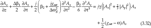
These equations are significant in the models relating to polarization states such as polarization mode dispersion in fiber transmission and nonlinear polarization rotation in passive-mode locking [7–9]. For an optical fiber with the length L, the phase variation of polarization components due to nonlinearity can be derived by considering the nonlinear term only in (3.32) through (3.33) for simplicity:

and hence the angle of polarization rotation is given by

Note that this angle is zero when the light input is linearly polarized due to |A_x|² = |A_y|². On the other way, the polarization ellipse rotates with propagation in the fiber.

3.3 Optical Solitons

3.3.1 Temporal Solitons

The NLS Equation (18.3) derived in Section 3.3.2 governs the propagation of optical pulse in nonlinear dispersive media such as optical waveguides or fibers. By using the transformation of variables as follows,

where τ₀ is a temporal scaling parameter often taken to be the input pulse width and is the dispersion length. Equation (18.3) can be normalized to the (1 + 1)-dimensional NLS equation as

where s = sgn(b₂) = ±1 stands for the sign of the group velocity delay (GVD) parameter that can be positive or negative, depending on the wavelength. The nonlinear term is positive (+1) for optical fibers but may become negative (–1) for waveguides made of semiconductor materials. Thus, there are two cases of basic propagation in optical fibers relating to the dispersion which is normally measured by the parameter

where the dispersion parameter D is expressed in units of ps/(nm.km). For the standard single-mode fiber, D is positive or GVD is anomalous at wavelengths >1.3 mm, and D is negative or GVD is normal at wavelengths shorter than 1.3 mm.

Because of two different signs of the GVD parameter, optical fibers can support two different types of solitons that are solutions of Equation (3.38). In particular, Equation (38.3) has solutions in the form of dark temporal solitons in the case of normal GVD (s = +1) and bright temporal solitons in the case of anomalous GVD (s = –1). These solutions can be found by the inverse scattering method [10]. In case of anomalous GVD, Equation (38.3) takes the form

and the most interesting solution of this equation is the fundamental soliton with the general form given by

Thus, at the input of the fiber, the soliton is given as and it can be converted into real units as follows:

Solution 3.42 indicates that if a hyperbolic-secant pulse with peak power P₀_, which satisfies expression 3.42, it can propagate undistorted without change in temporal and spectral shapes in an ideal lossless fiber at arbitrary distances as shown in Figure 3.1. This important feature results from the balance between GVD and self-phase modulation (SPM) effects. When a peak power launched into the fiber is much higher, a higher-order soliton can be excited with the input form

FIGURE 3.1
Evolution of (a) the first-order soliton and (b) the second-order soliton.

where N is an integer that represents the soliton order and is determined by

Different from the fundamental soliton, the temporal and spectral shapes of higher-order solitons vary periodically during propagation with the period or in real units .

With s = +1 in the case of normal GVD, Equation (38.3) takes the form

and solutions of (3.45) are dark solitons found by the inverse scattering method similar to the case of bright solitons. Solution of a fundamental dark soliton is given by [1,11]

The features of the dark soliton are a high constant power level with an intensity dip and an abrupt phase change at the center depending on parameter ϕ. For ϕ = 0, the dark soliton is a black soliton with the zero dip and a phase jump of π at the center. When ϕ ≠ 0, the dip intensity is nonzero and such solitons are called the gray solitons as shown in Figure 3.2.

In general, solitons in fiber have attracted a lot of interest in research from fundamentals to practical applications due to their unique features. In communication systems, the understanding of solitons is of importance in both transmission and signal processing [2,12].

FIGURE 3.2
(a) Intensity and (b) phase profiles of dark solitons for various values of the internal phase f.

3.3.2 Dissipative Solitons

Optical solitons mentioned above only exist in an ideal propagation medium that has no perturbations such as loss and gain. In practical systems such as mode-locked fiber lasers, the optical signal is periodically amplified to compensate the loss that it experiences in the fiber cavity. Thus, there is a periodic variation of the pulse power, which can form an index grating and induce modulation stability. It was demonstrated that solitons are able to exist in these systems [2]. Therefore, propagation of the optical pulse in this case should be described by the complex cubic G–L Equation (26.3) that includes the loss and gain effects. Similar to the NLS equation, it is useful to introduce the dimensionless variables and Equation (26.3) becomes

where

Because Equation (47.3) is not integrable, so a solitary wave can be guessed to give [2]

The parameters of the solution are determined by substituting it in Equation (47.3) and they are

Thus, the width and the peak power of the soliton are determined by the system parameters such as loss, gain, and its finite bandwidth. Different from solitons supported by the NLS equation, influence of these parameters plays an important role in the existence of solitons in these fiber systems. Due to periodic perturbations during propagation, solitons dissipate their energy that plays an essential role for their formation and stabilization. Such a soliton is often called a dissipative soliton or an autosoliton due to its mechanism of self-organization [5]. In order to preserve the shape and energy, a balance between gain and loss mechanisms is required in addition to the balance between GVD and SPM. A frequency chirping can help to maintain the balance between gain and loss during propagation in a bandwidth-limited system, and this explains why dissipative solitons are normally chirped pulses.

3.4 Generation of Solitons in Nonlinear Optical Fiber Ring Resonators

3.4.1 Master Equations for Mode Locking

Mode locking is a technique to force axial modes of a laser in phase to generate short pulses. For mode-locked fiber ring lasers, an optical pulse in every round-trip would experience the same effects such as loss and gain as that in a transmission fiber span. Thus, the circulation of the pulse inside the ring resonators is approximately equivalent to a propagation of the pulse in a fiber transmission link with infinite length. Therefore, Equation (26.3) can be used to describe mode locking in fiber lasers. However, the variation of the pulse in the round-trip time scale is considered rather than that in the distance scale. In addition, a modulation function M that is responsible for various mode-locking mechanisms is necessary to be added into (3.26). Then Equation (26.3) can be modified by introducing new variables, where v_g is the group velocity of the optical pulse, to obtain

A further modification is implemented by multiplication of both sides in (3.54) with L_c, the ring cavity length, and setting, which is the cavity period adding. Then (3.54) becomes

Equation (3.55) is the well-known master equation that was first derived by Haus to describe mode locking in the time domain [13]. Thus, there are two time scales in this equation: the time T is measured in terms of the cavity period or the round-trip time T_c, while the time τ is measured in terms of the pulse window. The term M, which depends on the mode-locking mechanism, passive or active, is a function of amplitude and time in terms of time scale τ in every round-trip. In most theoretical studies on mode locking, Equation (55.3) has been applied for the investigation of the pulse evolution in the cavity. We note that the parameters in the master equation are averaged over the cavity for analysis.

3.5 Passive Mode Locking

As mentioned in Chapter 1, there are three popular structures of the passive mode-locked fiber laser as shown in Figure 3.3. In the first structure, a saturable absorber acts as a passive mode locker to attenuate lower-intensity parts of a pulse, whereas higher-intensity parts of a pulse are minimally attenuated because they quickly saturate the absorber and pass through without loss (see Figure 3.3a). A saturable absorber is normally a semiconductor device that can be a bulk InGaAsP saturable absorber or a saturable Bragg reflector (SBR) based on InGaAs/InP multiple quantum wells. In some cases a mirror attached to the saturable absorber is also made using a periodic arrangement of thin layers that forms a grating and reflects light through Bragg diffraction. In practice, most SBRs are slow saturable absorbers because their response is much longer than the time scale of the pulse width. For the passive mode-locked fiber laser using SBR, the width of the mode-locked pulses is commonly of picoseconds time scale [14,15]; however, shorter pulses of less than 500 fs can be generated by careful dispersion management in the fiber cavity [16]. The second configuration is based on a nonlinear fiber loop mirror (NFLM), known as an all-optical switch. The NFLM is a Sagnac interferometer as described in Figure 3.4a whose intensity-dependent transmission can shorten optical pulses propagating inside the cavity. In passive mode-locked fiber lasers based on this configuration, the NFLM connects to a main fiber ring through a 3 dB coupler that splits the entering pulses into two equal counterpropagation parts as shown in Figure 3.3b. Because the optical amplifier is unequally located in the Sagnac ring, the counterpropagation pulses acquire different nonlinear phase shifts after a round-trip inside such a Sagnac loop. Moreover, the phase difference also depends on the temporal profile of the optical pulse; thus, the peak of the pulse is passed without loss while the pulse wings are reflected due to their lower intensity and smaller phase shift. It can be shown that the transmittance of the NFLM varies as a function of pulse power P via [17,18]:

FIGURE 3.3
Typical configurations of passive mode-locked fiber laser: (a) a linear cavity configuration, (b) a configuration based on nonlinear fiber loop mirror, and (c) a ring configuration based on nonlinear polarization rotation.

FIGURE 3.4
A description of operation and transmissivity of artificial fast saturable absorption based on (a,c) nonlinear fiber loop mirror (NFLM) and (b,d) nonlinear polarization rotation (NPR), respectively.

where G is the amplification factor and L is the length of the Sagnac loop. Thus, a complete transmission is implemented when the peak power P_p satisfies the condition:

In other words, the peak of the pulse experiences a higher net gain per round-trip than its wings to shorten the pulse. This mechanism is sometimes known as additive pulse mode locking (APM), and the NFLM can be considered as a fast or artificial saturable absorber as shown in Figure 3.4c. The fiber lasers using NFLM were first proposed for mode locking in 1991 with generated pulse-width of 0.4 ps [19] and a much shorter width of 290 fs was obtained from this laser by optimizing the dispersion and nonlinearity in the fiber cavity [20].

In the third configuration using nonlinear polarization evolution, the intensity-dependent change in the polarization state is explored for mode locking through a polarizing element. Figure 3.3c shows a setup of the passive mode-locked fiber laser based on this principle. The physical mechanism behind mode locking makes use of the nonlinear birefringence. A polarizer that can be also an isolator combined with two polarization controllers acts as a mode locker as described in Figure 3.4b. The polarizer makes the optical wave linearly polarized, and then the following polarization controller changes the polarization state of the wave to elliptical. The polarization state evolves nonlinearly during propagation of the pulse due to the nonlinear phase shift of two orthogonal polarization components in the birefringent fiber ring. The transmissivity of this structure is given by

where α is the angle between the polarization directions of the input light and the fast axis of optical fiber, φ is the angle between the fast axis of optical fiber and the polarization direction of the polarizer, and are linear and nonlinear phase differences between the two orthogonal polarization components, respectively. And they are given by

where n_x and n_y are the refractive indices of the fast and slow axes of the optical fiber, respectively, and L is the length of the fiber in the cavity. Because of the intensity dependence of the nonlinear phase shift in expression (3.60) as shown in Figure 3.4d, the state of polarization varies across the pulse profile. The polarization controller before the polarizer is adjusted to force the polarization to be linear in the peak of the pulse; hence, the high-intensity part passes the polarizer without loss while the lower-intensity wings are blocked. Thus, the pulse is shortened after every round-trip inside the fiber ring. This configuration can generate easily very narrow pulses of sub-100 fs by careful dispersion optimization [21–23]. The shortest pulse of 47 fs has been generated from the erbium-doped fiber laser by this technique [24].

In the above techniques, the ring configurations based on NFLM and NPR are normally applicable to soliton fiber lasers due to their fast response of the saturable absorption process as well as a possibility of self-initialization. A fast saturable absorption mode locking can be theoretically described by introducing the saturable loss modulation into the master equation (3.55). The modulation of a fast saturable absorber M_sa(t) can be modeled by [25]

where s₀ is the unsaturated loss, and I_sat is the saturation intensity of the absorber. In case of weak saturation (), expression (3.61) can be Taylor expanded to give

where s_SAM is called the self-amplitude modulation (SAM) coefficient. The master equation of passive mode locking thus can be derived by using (3.55) and (3.62):

We can simplify Equation (63.3) by incorporating the unsaturated loss s₀ into the loss coefficient and ignoring the effects of dispersion and nonlinearity:

This is the simplest case of passive mode locking where the pulse shaping is based on purely saturable absorption. The solution of (3.64) is a simple soliton pulse equation given by

By substitution of (3.65) into (3.64), the pulse width and relations between parameters of the system can be obtained [25]:

and

Expression (3.66) can explain why the pulse width in passive mode locking is much shorter than that in active mode locking due to the loss modulation and the curvature being proportional to, then the curvature of loss modulation increases faster when the pulse is shorter while it remains unchanged in active mode locking.

However, the effects of GVD and SPM are always significant to pulse shaping in practical passive mode-locked fiber lasers. Hence, the master equation needs to include these effects and is given by

This equation has a simple steady-state solution as follows [26]:

By using (3.69) as an anzat and balancing terms, the following pulse parameters and relations can be obtained as

Equation (3.71) indicates that a combination of anomalous GVD () and the SPM effect can give a zero chirp solution and the shortest pulses can be obtained in this case. For a small SAM coefficient and weak filtering, a soliton can be formed via the balance of anomalous GVD and SPM. The SAM and filtering effects can be considered as weak perturbations in the fiber cavity. However, they play an important role in stabilization of the pulse against noise build-up in the intervals between the pulses [25].

When solitons are periodically perturbed by the gain, loss, filtering, and SAM effects inside the fiber ring cavity, they radiate or generate continuum or dispersive waves. If the continuum components shed by the soliton are phase matched from pulse to pulse, its energy can build up and sidebands appear in the spectrum where the frequency components with the relative phase of soliton and dispersive wave change by an integer multiple (n) of 2π per round-trip. These parasitic sidebands were first described and explained by Kelly [27]. This phenomenon is observed in most passive soliton fiber lasers. The positions of sidebands in the spectrum depend strongly on the dispersion of the fiber cavity via [28]

where n is the order of sideband, D is the fiber dispersion parameter in the cavity, t_FWHM is the full width at half-maximum of the pulse and λ0 is the center wavelength. Thus, from the positions of sidebands in the obtained optical spectrum the dispersion of the cavity can be estimated.

3.6 Active Mode Locking

3.6.1 Amplitude Modulation (AM) Mode Locking

In AM mode locking, the amplitude modulation provides a time-dependent loss. The pulse will form at time slots where the loss dips are below the gain level. The modulation of an amplitude modulator can be mathematically described by

and the pulse evolution equation can be derived from general master Equation (55.3) to describe AM mode locking as follows:

where m_AM is the modulation index, and is the angular modulation frequency. For active AM mode locking, the modulation frequency is normally much higher and harmonics of the cavity fundamental frequency (f_c), with N being the order of harmonic.

In case of purely AM mode locking, we ignore the effects of GVD and SPM. Additionally, we can Taylor expand the modulation function to second order in time due to the pulse being positioned only at the minimum of the modulation curve. Then Equation (76.3) becomes

The solution of this equation is a Gaussian pulse given by

where

This is the result predicted by Kuizenga–Siegman [29], which shows the pulse width is proportional to the inverse of the gain bandwidth and the modulation frequency. The eigenvalue of the equation can give the important condition of the mode-locked laser through the expression

where and ; G and l parameters are considered as the gain and the loss within one round-trip of the fiber cavity. Thus, the expression (3.80) also indicates that the gain must be fixed at a certain value higher than the loss to compensate for the excess loss caused by the modulator and the filtering from the limited gain bandwidth. This condition requires that the gain be sufficient for compensating the loss of the ring cavity. Optical fiber amplifiers are thus preferred to operate in the saturation region in the cases when the ring is either under modulation or no modulation states, so as to achieve stability of the total energy distributed in the ring.

With presence of the GVD effect in the fiber lasers, the evolution of the pulse inside the fiber ring cavity satisfies the following equation:

This is a Hermite’s differential equation, and a stable solution of this equation takes the form [25]

This is a chirped Gaussian pulse with the pulse parameters obtained by balancing terms in (3.81):

The result shows that if β₂ = 0 (ignoring GVD effect), then the chirp factor q = 0 and k = 0, and subsequently, the pulse width in (3.83) returns to (3.79). Thus, the presence of GVD can cause the generated pulse chirped.

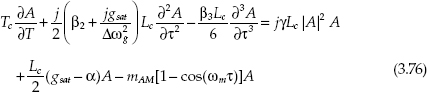
When the fiber cavity is pumped with sufficiently high power, the SPM effect is not negligible and included in the master equation as fully described in (3.76). With the addition of sufficient negative GVD and SPM, the solitary pulse formation can be obtained, and the solution of (3.76) is assumed to be a chirped secant hyperbole pulse [30]:

In a nonlinear regime, the pulse is shortened by a combination of SPM and negative GVD similar to passive mode locking. However, in order to shorten the pulse by soliton compression, the following two conditions must be satisfied [31]:

• The synchronization between the modulator and the pulse train must be maintained or the solitons must be exactly retimed on each round-trip. This is a common condition for stable operation of mode-locked fiber lasers against the thermal drift of the cavity length. This condition also ensures the phase matching requirement that is the total phase of the lightwaves circulating in the ring cavity must be a multiple number of 2π.

• The excess loss of the continuum determined by the eigenvalue of (3.76) must be higher than that of the soliton. The resulting condition is [32]

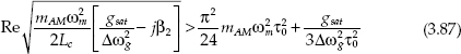
In (3.87), on the right side is the loss experienced by the soliton, and on the left side is the loss of the continuum. In addition, the modulation must not drive the soliton unstable. The condition for suppression of energy fluctuations of the soliton can be obtained from soliton perturbation theory [31–33]:

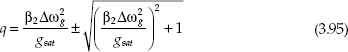
From the above conditions, the mode-locked pulse can be compressed with the width much shorter than that predicted by Kuizenga–Siegman. The factor of pulse width shortening R can be found as follows [34]:

The condition (3.89) determines the lower limit of the pulse width with the help of SPM and negative GVD. The possible pulse width reduction is proportional to the fourth root of dispersion that indicates the need for an excessive amount of dispersion to maintain a stable soliton while suppressing the continuum.

3.6.2 Frequency Modulation (FM) Mode Locking

In contrast to AM mode locking, FM mode locking is based on a periodic chirping caused by phase modulation. When the modulation frequency is exactly harmonics of the fundamental frequency, the phase matching condition is satisfied for resonance of optical waves in the cavity. In the frequency domain, the sidebands generated by phase modulation are matched to the axial modes of the cavity. While in the time domain, the pulses are built up at the extremes of the modulation cycles. At these temporal positions, the optical waves are not chirped and thus the optical waves are constructively summed when they are in phase, while they are destructively interfered at other temporal positions due to repeated linear chirping in the cavity.

A phase modulation of the optical field can be given by the function

where m_FM is the phase modulation index. When using the expression of phase modulation for a mode locker, an FM mode locking can be described by the master equation as follows:

Because the pulse is formed in only the narrow part of the modulation period, the modulation function can be approximated to the second order of the Taylor expansion. Then Equation (91.3) can be simplified by ignoring the nonlinear effect:

Therefore, Equation (92.3) describes the FM mode locking in a linear regime. Similar to AM mode locking, the solution of this equation is a chirped Gaussian pulse with the form

By the same techniques as in previous sections, the pulse parameters can be obtained:

In the simplest case—that is, the pure FM mode locking with β₂ = 0, the generated pulse is always chirped with q = ±1 due to phase modulation. On the other way, the pulses generated from a FM mode-locked laser can be located at either extreme up-chirp (q > 0) or down-chirp (q < 0) of the modulation cycle in the absence of dispersion and nonlinearity that can create a switching between these two states in a random manner [29]. However, in the presence of the dispersion effect, this switching can be suppressed as possibly indicated in (3.97), which is the expression of the excess loss of the cavity. If β₂ < 0 (anomalous dispersion), the excess loss at up-chirp half cycle is lower than that at down-chirp cycle (q > 0) and vice versa. Thus, the pulses located at positive half-cycles are preferred in the anomalous dispersive fiber cavity while those located at negative half-cycles are preferred in the normal dispersive fiber cavity. On the other hand, the pulse in the up-chirp cycle is compressed by the dispersion while the down-chirp pulse is broadened in the anomalous GVD cavity. This shortened up-chirp pulse experiences less chirp after passing the phase modulator, which reduces the loss due to the filtering and gains bandwidth limitation effects. The up-chirp pulse is finally dominant in the anomalous GVD cavity. This stability of the mode-locked pulse in the FM fiber ring laser has been theoretically demonstrated [35].

In a nonlinear regime, the SPM is also significant in pulse shaping. Similar to AM mode locking, the soliton is formed inside the fiber cavity with the balance between GVD and SPM effects. To generate stable solitons, the required gain for noise must be higher than that for the soliton, and the condition for stability can be obtained by the perturbation soliton theory [36]:

In Equation (98.3) the left side is the loss of the amplification stimulated emission (ASE) noise and the right side is the loss of the soliton. Tamura and Nakazawa [35,37] also indicated that the pulse energy equalization occurs in the support of SPM and the filtering effect when the dispersion of the cavity is anomalous. This stability of the soliton in the presence of the third-order dispersion in an FM mode-locked fiber laser has been numerically investigated in [38].

Besides the synchronous mode locking in an FM mode-locked fiber laser, another mechanism for mode locking based on asynchronous phase modulation has been proposed [39]. In this scheme, asynchronous modulation is obtained by detuning of modulation frequency with a proper amount. However, in order to generate a stable soliton train, the detuning is required to remain within a limit that satisfies the following condition [36]:

With a small detuning within this limit, the soliton can overcome the frequency shift to remain the mode-locked state. When the detuning exceeds the above limit, the noise can build up and destroy the solitons. The fiber laser will operate in an FM oscillation state if the modulation frequency is moderately detuned. In this regime, the output has a constant intensity in the time domain but with periodical chirp, and its optical spectrum is largely broadened [40]. The transition from FM oscillation state to phase mode locking has complex behavior at smaller detuning where the relaxation oscillations can occur with different properties [41]. In this state, the noise can build up faster than the soliton to become the new pulse and replace the old one. The cause of relaxation oscillation is the change of the cavity loss when the modulation frequency is detuned. The pulse passes through the modulator with a small time shift from the extremes of the modulation cycles that increase the loss of the pulse while the ASE noise gets more gain at the extremes of modulation cycles where they have the lowest loss in the cavity. When the detuning becomes larger, a new pulse can build up from the ASE noise while the old pulse decays and disappears finally. This process is periodically repeated and this repetition can satisfy the phase-matching condition for resonance in the fiber ring cavity, which leads to the relaxation oscillation. In this state, the output is periodically strong spikes but with lower average power because more power is stored in the cavity from resonance. The relaxation oscillation can occur several times due to the central mode hopping in the detuning process. The supermode noise can be dramatically enhanced between these transitions by getting the excess energy from the cavity through matching between the relaxation oscillation frequency and the frequency of beatings between the modulation sidebands and lasing modes [42]. All interesting phenomena exist only in the FM mode-locked lasers, and those have been theoretically and experimentally investigated [40–42].

3.6.3 Rational Harmonic Mode Locking

In active mode locking, there is one way to increase the repetition rate—use the rational harmonic mode locking with detuning the modulation frequency to a rational number of the cavity fundamental frequency [43]:

where N, M are integers; N is the harmonic order, and M can be considered as the multiplication factor.

To understand the rate multiplication in rational harmonic mode locking, a simple description in the frequency domain is shown in Figure 3.5a. In the frequency domain, the harmonics of modulation frequency would only be matched to the different multiples of the cavity modes when the modulation frequency is detuned with amount of f_c/M. Then the repetition rate of the output pulse can be multiplied by a factor of M. The mechanism can be understood in the time domain as described in Figure 3.5b. When the fiber laser is detuned by a ratio f_c/M, the difference between the cavity round-trip time and N times the modulation frequency is equal to the time delay experienced by a pulse after one round-trip. In another way, the phase delay of a pulse between consecutive round-trips is proportional to 2piN/M and the pulse returns to its original positions after M round-trips. As a result, there are M sets of pulses in one round-trip window resulting in a multiplied repetition rate.

FIGURE 3.5
A description of rational harmonic mode locking (a) in frequency domain, (b) in time domain with N = 2 and M = 3 as an example.

Because of the pulse distribution over a nonuniform modulation window, the output pulses suffer from large amplitude fluctuations that limit the application of rational harmonic AM mode locking in practical systems. Several methods such as nonlinear optics methods [44,45] and modulator transmittance adjustment [46–48] have been proposed for pulse amplitude equalization.

For the FM mode locking, the situation is different from the AM mode locking when it has been shown that the rational harmonic mode locking is due to the contributions of harmonics of the modulation frequency in the amplified electrical driving signal [49]. The higher-order harmonics are generated from the power amplifier operating in a saturated scheme. Therefore, the phase of the optical field at the output of the phase modulator can be modulated via

where E_in, E_out are the optical field at the input and output of the phase modulator, respectively, and j(t) varies corresponding to the driving signal. In case of the amplified signal, this variation can be represented by a summation of a series of cosine functions as follows:

where f_m is the modulation frequency, m_k and θ_k are the modulation index and the phase delay bias for each frequency component, respectively. From analysis in [49], the field of the optical signal experiences average phase modulation after M round-trips by

Thus, when the modulation frequency f_m is detuned as specified in Equation (3.100), the modulation effect of lower-order harmonics of the f_m are cancelled, and only the frequency component of M times the modulation frequency is enhanced and becomes dominant after M round-trips. In another way, the effective phase modulation curve with the number of cycles multiplied by M times in the same transmission window is proven in Figure 3.6. Because of mode locking based on frequency chirping, the generated pulse train in FM rational mode locking does not suffer from an unequal amplitude problem.

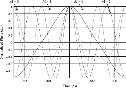
FIGURE 3.6
Average phase modulation profile at different detuning f_c/M with M = 1 ¸ 4 to achieve rational harmonic mode locking in the frequency modulation mode-locked fiber laser. The driving signal of the phase modulator is modeled with magnitudes of higher harmonic components as follows: m₂ = 0.008 m₁, m₃ = 0.06 m₁, m₄ = 0.001 m₁ and m₅ = 0.0008 m₁.

3.7 Actively Frequency Modulation Mode-Locked Fiber Rings: Experiment

3.7.1 Experimental Setup

By using an electro-optic phase modulator as a mode locker, the active mode-locked fiber ring laser can generate a high-speed pulse train with low jitter. Moreover, it is simple in synchronization between the fiber cavity and other electronic devices. In this section, an active FM mode-locked fiber ring laser will be constructed for demonstration of soliton generation at a high repetition rate in which the erbium gain medium is used for amplification inside the cavity.

Figure 3.7 shows the experimental setup of the FM mode-locked fiber ring laser. In this setup, an erbium-doped fiber amplifier (EDFA) pumped at 980 nm is used in the fiber ring to moderate the optical power in the loop for mode locking. This amplifier operates in the saturation region, and the output power can be adjusted by varying the pump power or the current of the pump laser diode. A 50 m Corning SMF-28 fiber is inserted after the EDFA with the aim of enhancing the nonlinear phase shift through the SPM effect as well as ensuring that the average dispersion in the fiber ring is anomalous, which is important in designing a stable soliton fiber laser. By measuring the input and output power of the EDFA, the total loss of the cavity can be estimated. This loss, consisting of the insertion loss of the phase modulator and connections, is approximately 10.5 dB to 11 dB in our setup. We note that the loss can vary due to the change in the polarization state.

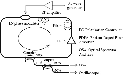
FIGURE 3.7
Experimental setup of the active frequency modulation mode-locked fiber laser.

An electro-optic integrated phase modulator PM-315P of Crystal Technology, Inc. of Sunnyvale, California, United States, assumes the role as a mode locker and controls the states of locking in the fiber ring. At the input of the phase modulator, a polarization controller (PC) consisting of two quarter-wave plates and one half-wave plate is used to control the polarization of light, which is required to minimize the loss cavity and influences the stable formation of solitons. The phase modulator with half-wave voltage of 9 V is driven by a sinusoidal signal generated from a signal generator HP-8647A in the region of 1 GHz frequency. The radio-frequency (RF) sinusoidal wave is amplified by a broadband RF power amplifier DC7000H with 18 dB gain, which can provide a maximum saturated power of approximately 19 dBm at the output. Thus, the phase modulation index of ~1 radian can be achieved for mode locking. The fundamental frequency of the fiber laser cavity is determined by tuning the modulation frequency to lock the fiber laser at different harmonics. In our setup the fundamental frequency of the fiber cavity is 2.2862 MHz, which is equivalent to the 90 m total length of the fiber ring.

The outputs of the mode-locked laser extracted from the coupler 90:10 are monitored by an optical spectrum analyzer HP-70952B and an oscilloscope Agilent DCA-J 86100C with an optical bandwidth of 65 GHz. Because of the fiber laser operating at only 1 GHz, bandwidth of the oscilloscope is wide enough for pulse width measurement larger than 10 ps. In case of the pulse with the width less than 10 ps, the rise time of the oscilloscope, which is 7.4 ps, should be considered in the estimation of the pulse width as where τ_p, τ_meas and τ_equi are the estimated and measured pulse widths and the rise time of the oscilloscope, respectively. An RF spectrum analyzer FS315 is also used to determine the stability of the generated pulse train.

FIGURE 3.8
Experimental setup of the active mode-locked fiber laser using phase-modulated Sagnac loop (PMSL). (a) A whole fiber ring laser. (b) Detailed diagram of the PMSL.

Besides the conventional ring structure as described above, another setup of the active mode-locked fiber ring laser using electro-optic (EO) phase modulator, which is based on the Sagnac loop interferometer polarization maintaining Sagnac loop (PMSL) and also was implemented in our experiment. When the phase modulator is placed at the middle of a fiber Sagnac loop as shown in Figure 3.8, phase modulation is converted into amplitude modulation by interference between clockwise light and counterclockwise light, which have a phase difference between them. This effect comes from the fact that the phase modulator is optimized for only one transmission direction. The transmission of the PMSL output is given by [50]

where Dφ(t) is the differential phase caused by the driving signal between two passage directions, and ϕ is the bias differential phase.

Thus, in this configuration of the active mode-locked fiber laser, the PMSL can be considered as an amplitude modulator without the bias drift problem and possibly polarization dependence [50,51]. Expression (3.104) shows that the intensity modulation of the PMSL can operate at double modulation frequency. However, the mode-locked pulses at peaks of the transmission acquire residual chirp from phase modulation [52]. This chirp will affect the pulse characteristics as well as stability in the same way as in the active FM mode-locked fiber ring laser. Similar to the rational mode locking, the repetition rate multiplication can be archived by detuning with a different rational number of harmonics. The detuning allows the pulses to experience the opposite chirp in consecutive round-trips and consequently, a uniform intensity transmission window can be obtained. In fact, the intensity modulation curve of the PMSL depends strongly on the phase modulation profile. If the phase modulation curve is distorted, the higher-order harmonics in the resulted intensity modulation signal are also strongly enhanced to facilitate the rational harmonic mode locking.

3.7.2 Results and Discussion

3.7.2.1 Soliton Generation

By setting the saturated power of the EDFA of 5 dBm, a stable pulse train is generated by tuning the modulation frequency at the 438th-order harmonics of the fundamental frequency. Figures 3.9a through 3.9c show the time trace and spectrum of the generated mode-locked pulse. The temporal and spectral widths of the pulse are 12.5 ps and 0.23 nm, respectively. Thus, this result indicates that the pulse is transform limited with the product of time-bandwidth of 0.36. Because no optical band-pass filter is used in the setup, the emission wavelength of the fiber laser is around 1560 nm where the gain of the EDFA is maximized and flat after optimizing the polarization state of the cavity. Stability of the mode-locked pulse train is demonstrated by the RF spectrum analysis as shown in Figure 3.9d. The sideband suppression ratio (SSR) of higher 50 dB was achieved without any feedback circuit for stabilization.

FIGURE 3.9
Time traces of (a) the pulse train, and (b) the single pulse, (c) corresponding optical spectrum, (d) radio-frequency spectrum of the mode-locked pulse generated from the frequency modulation mode-locked fiber ring.

FIGURE 3.10
(a) Time trace and (b) spectrum of the mode-locked pulse generated from the FM mode-locked fiber ring laser using the phase modulator Mach-40-27.

With the aim of increasing in the phase modulation index, we replaced the phase modulator PM-315P by the phase modulator Covega’s Mach-40-27, which has a half-wave voltage of only 4 V at 1 GHz modulation frequency. It is surprising that a larger width of generated pulses at the higher modulation index of 2.3 rads was obtained in this setup with the same intracavity optical power as in the previous setup. Figure 3.10 shows the time trace and the corresponding optical spectrum of the mode-locked pulse generated from this setup. The pulse broadening in this case indicates a limitation of pulse spectrum or gain bandwidth in the cavity that can relate to the property of the phase modulators and would be examined to explain more detail in Chapter 4.

In the configuration of the mode-locked fiber laser using PMSL, the generated pulse train has a high stability but wide pulse width. Figure 3.11 shows the time trace of the pulse train at 1 GHz generated from this configuration. Because of the insertion of the 3 dB coupler in the PMSL, the total loss of the ring cavity is about 16 dB, which is much higher than that of the conventional FM mode-locked fiber ring laser. High cavity loss reduces the efficiency of the soliton compression effect in the fiber laser. Additionally, the PMSL is equivalent to an amplitude modulator, so that the modulation index depends on the intensity modulation curve converted from the phase modulation. With a small phase modulation index, the modulation index of the PMSL is also small. Therefore, the width of the generated pulse is about 100 ps, and the pulse shape is a Gaussian pulse rather than a soliton.

FIGURE 3.11
Time trace of the pulse train generated from the mode-locked fiber laser using phase-modulated Sagnac loop.

3.7.2.2 Detuning Effect and Relaxation Oscillation

When the modulation frequency f_m is detuned, the fiber laser can experience various regimes. Especially, the transition state shows complex behaviors such as relaxation oscillation and excess noise enhancement. In our setup, the fiber laser experiences three main regimes that consist of the mode-locked regime, FM oscillation, and transition regimes depending on detuning amount. fBecause the range of in each regime depends on the cavity length or the cavity dispersion, we inserted 100 m SMF-28 fiber into the fiber ring (case A) beside 50 m SMF-28 fiber in the original setup (case B). By detuning the FM, the important regimes in both cases are identified as follows:

FIGURE 3.12
Optical spectra at different frequency detuning regimes: (a) frequency modulation oscillation, (b) entering the transition regime, (c) enhanced relaxation oscillation in the transition regime, and (d) relaxation oscillation at higher optical power level.

• When for the case A and for case B, the fiber ring laser operates in an FM oscillation regime that can be identified by its optical spectrum. At large the optical spectrum is similar to a CW signal due to the limitation of resolution in optical spectrum analyzer (OSA), while the RF spectrum cannot identify the first harmonic component of f_m as shown in Figure 3.14a. When the effective modulation index is sufficient by decreasing the optical spectrum is broadened with a double-peak shape due to the energy going to the optical frequencies far from the center carrier mode as shown in Figure 3.12a. The spectrum keeps broadening when the decreases close to 2 kHz and 4 kHz for the cases of and, respectively. Figure 3.14b also shows the typical RF spectrum in this regime, which indicates a strong supermode noise and a broad line-width of each side mode due to the beating between the cavity modes and the modulation frequency. Moreover, the strength of the first harmonic is increased according to the reduction of .

FIGURE 3.13
Time traces in the transition regime: (a) at initial stage and (b) at latter stage when the relaxation oscillation is enhanced.

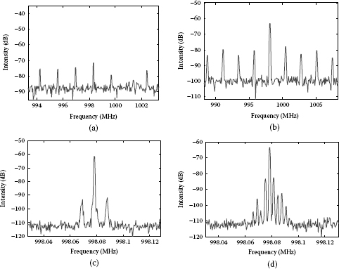
FIGURE 3.14
Radio-frequency spectra at different regimes: (a) continuous-wave-like regime, (b) frequency modulation oscillation regime and transition regime in span of 20 MHz, (c) initial stage of transition regime in span of 100 kHz, and (d) enhanced relaxation oscillation in transition regime in span of 100 kHz.

• When for case A and for case B, the fiber laser enters a transition regime where many complex behaviors such as the relaxation oscillations as well as the enhanced supermode noise status can occur [42]. The double-peak spectrum broadening becomes maximum before the energy at the main carrier grows up according to the reduction of detuning as shown in Figure 3.12b. Between the FM oscillation and mode-locking regimes, the relaxation oscillations (RO) as well as the enhanced supermode noise status have also been observed. In the first stage, the time trace shows a high constant intensity that varies continuously and rapidly in the time domain. When the detuning deceases further, the envelope of high intensity is more deeply modulated as shown in Figure 3.13a. Because the supermode noise is still the dominant noise source, the RF spectrum exhibits behavior similar to that shown in Figure 3.14b. In a narrower resolution bandwidth, the beat noise between the modulation sidebands and the cavity modes of about 10 kHz can be observed as in Figure 3.14c. In the latter stage of the transition regime, when the detuning is decreased to around 500 Hz, the RO becomes stronger as an enhanced excess noise. In this state, the building up of new pulses and the decay of old pulses can occur at the same time that a rapid variation of both amplitude and time position is exhibited. Therefore, in this state the time trace of the signal is observed as noisy pulses as shown in Figure 3.13b and the corresponding optical spectrum show ripples in the envelope as shown in Figure 3.12c. If the optical power in the cavity is further increased, the optical spectrum can exhibit sidebands as seen in Figure 3.12d, which indicates the existence of ultrashort pulses with high peak power in this stage. Figure 3.14d shows the RF spectrum with strong sidebands of 2 kHz formed by beating between the modulation frequency and the RO frequency.

• When for the case A and for the case B, the mode-locked state can be achieved. When the detuning is decreased to a small amount that is within a specific limitation as specified in (3.99) or no detuning, the mode locking can be achieved to generate the stable pulse train as shown in Figure 3.9. By providing a sufficient gain in the cavity the RO noise suppression greater than 40 dB and the supermode noise suppression greater than 45 dB can be achieved in our setup without using any stabilization technique.

In the transition regime, it is really interesting that the existence of ultrashort pulses with very high peak power is observed in this regime when the detuning is about 500 Hz incorporating with the adjustment of the polarization controller. Figure 3.15 shows the spectrum and the time trace of this state in case of A. In this figure the time trace shows the generated pulses with very narrow width and fixed high peak power but strong timing jitter, while the optical spectrum shows a broad spectral width and Kelly sidebands generated by the resonance of dispersive waves and the generated pulses. These results indicate clearly the existence of solitons in this state. Based on the spectral width of 1.58 nm, the pulse width is approximately 1.8 ps, which is impossible to be obviously resolved by the oscilloscope. From the sideband locations, the total cavity dispersion estimated by (3.74) is of about –0.0172 ps²/m. High stability of the optical spectrum also demonstrates that solitons are stably formed inside the cavity. We believe that the passive mode locking based on NPR plays a key role in this state. This process can be explained as follows: when the cavity is slightly detuned, the relaxation oscillation occurs in which pulses in the form of spikes acquire such high peak power that the NPR becomes significant in the weak birefringence cavity. In a favorable condition by changing the settings of the polarization controller, the passive mode locking based on NPR can be achieved to shape the pulse circulating in the cavity. Thus, the fiber laser in this state operates similar to a hybrid passive-active mode-locked laser [53–55]. In order to verify this passive mechanism the RF modulation signal was turned off; however, the optical spectrum with sidebands remained at least 5 minutes before it disappeared. Owing to the detuning, solitons experience a frequency shift that results in temporal variation of the pulses or timing jitter. Moreover, this state operates in the additive-pulse mode locking (APM) regime, and it is easily prone to dropout as demonstrated in Figure 3.15b by the baseline at the bottom of the pulse trace. This state is also observed in case B, although it is more difficult for adjustment due to an insufficient NPR effect in a shorter fiber cavity. By carefully adjusting the polarization controller, solitons generated by this mechanism in case B can be obtained as shown in Figure 3.16. With the first sideband spacing of 3.95 nm, the estimated average GVD of the cavity is about –0.0144 ps²/m. The estimation of the average GVD is valid due to a reduction of the dispersion in case B of –1.1 ps², which is exactly equivalent to the 50 m SMF-28 fiber.

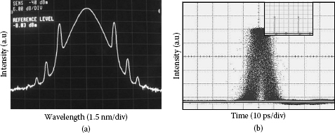
FIGURE 3.15
Spectrum and time trace of the hybrid mode-locking state in the case A with an insertion of 100-m SMF-28 fiber into the ring cavity: (a) observed spectrum and (b) recorded domain pulse and jittering.

FIGURE 3.16
Spectrum and time trace of the hybrid mode-locking state in the case B with an insertion of 50-m SMF-28 fiber into the ring cavity: (a) observed spectrum and (b) time domain pulse.

3.7.2.3 Rational Harmonic Mode Locking

As described before, a rational harmonic mode locking can be implemented in the active FM mode-locked fiber laser by the higher-order harmonics of the amplified driving signal. By using an RF spectrum analyzer, the magnitude of the harmonics at the output of the power amplifier is measured as a function of the RF input power. Figure 3.17 shows the measured results that indicate a strong increase of the second harmonics while the magnitude of the first-order harmonic remains unchanged at saturated value of 19 dBm at the RF input power higher than 2 dBm. Higher-order harmonics such as the third- and fourth-order harmonics are slightly enhanced at the input power higher than 5 dBm. The magnitude of high-order harmonics determines the modulation index of the rational harmonic mode locking at corresponding orders.

When the modulation frequency is detuned by the amount of ±f_c/2 and ±f_c/3 from the 438th harmonics of the cavity frequency, pulse trains at the repetition rate of double and triple modulation frequency are generated as shown in Figure 3.18 at the RF input power of 7 dBm. The pulse train at the second-order rational harmonic mode locking shows a better performance than that at the third-order rational harmonic mode locking due to the higher modulation index of the second harmonic component. Other rational harmonic mode locking such as the fourth and the fifth orders also can be obtained by an appropriate detuning but give very poor performance due to weak strength of the corresponding harmonic components in the driving signal.

FIGURE 3.17
Output power of the first, second, and third harmonics as a function of the radio-frequency input power.

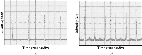
FIGURE 3.18
Time traces of the pulse trains in (a) the second- and (b) the third-order rational harmonic mode locking.

Similarly, the rational harmonic mode locking can be achieved in the mode-locked fiber laser using PMSL. Although the phase modulator operates in the small signal modulation region, the higher-order harmonic components in amplitude modulation of the PMSL can be easily enhanced by the distortion of phase modulation through phase-amplitude conversion. By detuning the modulation frequency of ±f_c/M with M from 2 to 6, the repetition rate of the pulse train is multiplied by a factor M as shown in Figure 3.19. However, the amplitude of pulses is unequal because of the nonuniformity of the intensity modulation profile.

Thus, the pulse trains at the output of the mode-locked fiber ring laser using PMSL show the problem of nonuniform amplitude, which is a disadvantage of the rational harmonic mode locking using amplitude modulation. The uniform pulse trains are always generated by phase modulation in rational harmonic mode locking if the strength of higher-order harmonic components is sufficiently high in the driving signal.

3.8 Simulation of Active Frequency Modulation Mode-Locked Fiber Laser

3.8.1 Numerical Simulation Model

Although an FM mode locking can be theoretically described by the master equation with averaged parameters, it is difficult in solving this equation to find an analytical solution with involvement of all important effects. Therefore, in order to understand the physical processes occurring inside the fiber ring cavity, a numerical model is developed in this chapter. The model of a mode-locked fiber laser with a ring configuration consists of basic components similar to that in the experimental setup. Figure 3.20 shows the block diagram of the numerical model for an active FM mode-locked fiber ring laser. In this model, a slowly varying envelope of the optical pulse passes through each component once in each round-trip. This process will be repeated until a desired solution is obtained. Thus, the envelope function of the pulse at the nth round-trip can be given by

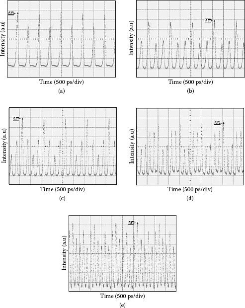
FIGURE 3.19
Time traces of (a) the second-order, (b) the third-order, (c) the fourth-order, (d) the fifth-order, and (e) the sixth-order rational harmonic mode locking in the fiber ring laser using phase-modulated Sagnac loop.

where Aⁿ, A^n-1 are the complex amplitudes of the pulse at the nth and the (n – 1) th round-trips, respectively; ,,and are the operators representing the loss of the cavity, the modulation mechanism, and the passive and active fibers, respectively. Based on well-understood physical mechanisms, the operators or the models of the components inside the ring cavity can be exactly as described and the effect of each component is individually considered in the model.

First, the operators and that describe propagation of the optical field in optical fibers can be modeled by the generalized NLS equation (3.26), which can be rewritten for convenience as follows:

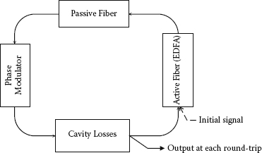
FIGURE 3.20
Numeric model for an active frequency modulation mode-locked fiber ring laser.

In case of passive fiber, the gain factor is set to zero, but the gain factor with saturation is nonzero in active fiber for amplification in the EDFA and modeled by using Equations (3.23) and (3.25). The ASE noise generated from the EDFA is also included at the end of the active fiber. The ASE noise is modeled as an additive complex Gaussian-distributed noise with a variance given by

where h is Planck constant, is the optical carrier frequency, G is the gain co-efficient and B_ASE is the optical noise bandwidth, and n_sp is the spontaneous factor that relates to the noise figure NF of the EDFA as follows:

Equation (3.106) for both active and passive fibers can be solved by using the well-known split-step Fourier method in which the fiber is split into small sections of length and the linear and nonlinear effects are alternatively evaluated between two Fourier-transform domains, respectively [1].

Second, the operator for an EO phase modulator is given by

where m is the phase modulation index, f₀ is the initial phase, and ω_m = 2πf_m is the angular modulation frequency, assumed to be a harmonic of the fundamental frequency of the fiber ring, Dt_s is the time shift caused by detuning and given by

where is the modulation period, with T_c is the cavity period and N is the harmonic order, and T is the time scale in terms of the round-trip scale.

Besides the attenuation of optical fibers, there are some losses inside the cavity such as coupling loss and insertion losses of the modulator and connectors. All these losses need to be included in the simulation and combined into the total cavity loss factor. The influence of this loss is given as

where l_dB is the total loss of the cavity in dB. Thus, this effect in turn determines the required gain coefficient of the EDFA to ensure that the gain is sufficient to compensate the total loss in a single round-trip for stable lasing operation.

Equations (3.106) through (3.111) provide a full set of equations for numerical simulation of an active FM mode-locked fiber ring laser. Due to the recursive nature of pulse propagation in a ring cavity, operation of the operators is repeatedly applied to the complex envelope of the pulse to find a stable solution. The complex amplitude of the output is used as the input of the next round-trip and stored for display and analysis. In simulation of pulse formation, a complex Gaussian-distributed noise of –10 dBm is used as a seeding signal. Depending on the strength of the effects in the model, a stable pulse can be found in 500 round-trips or even up to 10,000 round-trips. The number of samples in the simulation window as well as the step-size in the spatial domain is properly chosen to minimize numerical errors in calculation.

TABLE 3.1
Parameter Values Used in Simulations of the Frequency Modulation (FM) Mode-Locked Fiber Laser

3.8.2 Results and Discussion

3.8.2.1 Mode-Locked Pulse Formation

By using the numerical model described above, the pulse formation in the FM mode-locked fiber ring laser can be investigated. Table 3.1 summarizes all parameters used in the simulations. Figure 3.21a shows an evolution of the mode-locked pulse built up from the noise at m ~ 1 radian in the ring cavity with an anomalous of –0.0171 ps²/m. Figure 3.21b plots the peak power as a function of round-trip number. The steady state is only reached after 5000 round-trips, and a damped oscillation occurs in the initial stage of the pulse formation process. Figure 3.22 shows the time trace and the spectrum of mode-locked pulse at steady state. We note that the pulse with the width of 11.6 ps is well fitted to a secant hyperbolic pulse rather than a Gaussian pulse. However, its spectrum exhibits no sideband due to weak dispersive waves in the cavity.

FIGURE 3.21
(a) Numerical simulated evolution of the mode-locked pulse formation from the noise, (b) variation of the peak power 5000 round-trips in the anomalous average dispersion cavity.

FIGURE 3.22
(a) Numerical simulated time trace and (b) the corresponding spectrum of mode-locked pulse at steady state in the anomalous average dispersion cavity.

The effect of the phase modulation index m on the mode-locked pulse is also numerically investigated by varying the index in a range from 0.175 rad to π rad, and the results are shown in Figure 3.23. The increase in modulation index shortens the pulse width. At the index lower than 0.5 rad, the rate of pulse shortening is higher due to the soliton compression effect that results from the dominant SPM effect in pulse shaping. However, at the modulation index higher than 0.5 rad, where the active phase modulation becomes stronger in pulse shaping, the reduction of the pulse width is slow and almost linear. The chirp of pulse is increased with the increase in the phase modulation index, and the pulse diverges from the secant hyperbolic profile and closer to a Gaussian pulse at a higher index. Figure 3.24 shows the waveforms of the generated pulse at two different modulation indices with the Gaussian fit and secant hyperbolic fit curves.

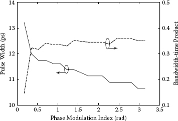
FIGURE 3.23
Variation of mode-locked pulse parameters as a function of the phase modulation index in the anomalous average dispersion cavity.

FIGURE 3.24
Numerical simulated waveforms in steady state of mode-locked pulses at two different modulation indices (a) m = 0.87 radian, and (b) m = π radian.

Instead of an anomalous dispersion cavity, the sign of dispersion in the fibers is reversed to provide a normal dispersion cavity with of +0.0213 ps²/m. With the same conditions of mode locking, the mode-locked pulse in the normal dispersion cavity is wider than that in the anomalous dispersion cavity. The parameters of the mode-locked pulse as a function of the modulation index in the normal dispersion cavity are depicted in Figure 3.25. The pulse is also shortened with the increase in the phase modulation index. Evolution of the mode-locked pulse in the normal average dispersion cavity at m ~ 1 radian is shown in Figure 3.26a. Figure 3.27 shows the pulse profile in the time domain and its spectrum is steady state, which indicates a parabolic pulse rather than a soliton or Gaussian pulse. Furthermore, in the initial stage of pulse formation, there is an existence of dark soliton embedded into the background pulse growing up as shown in Figure 3.26b. It is understood that in this stage the accumulated phase modulation is relatively weak, so that the SPM effect is dominant due to the high gain from the EDFA. The dark soliton formation occurs from the balance of normal GVD and SPM effects, yet the dark soliton is unstable. It experiences a periodic variation of time position (dotted line in Figure 3.26b) and decays due to the chirping caused by active phase modulation. Figure 3.28 shows the waveform with a dip at near center of the background pulse and its phase profile with a phase change of about π/2 at the dip at the 2900th round-trip. Because the intensity of the dip that also varies along the evolution is nonzero, the formed dark soliton is referred to as the gray soliton rather than the black soliton. The existence of a dark soliton remains only until the accumulated phase shift is sufficient to lock a pulse at the minimum of modulation cycle.

FIGURE 3.25
Variation of mode-locked pulse parameters as a function of the phase modulation index in the normal average dispersion cavity.

In the FM mode-locked fiber laser, the pulse formation at up-chirping or down-chirping cycles depends on the dispersion of the cavity, which is anomalous or normal. On the other way, the pulse switching between positive and negative modulation cycles is suppressed due to the presence of the GVD effect. Figure 3.29 shows evolutions of the mode-locked pulses built up from noise in normal and anomalous dispersive fiber rings in one modulation period. The modulation curve is phase shifted by π/2 to display both up-chirp and down-chirp cycles in the same simulation window. The dashed lines in the graphs indicate the phase modulation curve applied in every round-trip. Thus, the pulse is built up only at the extreme of the up-chirp cycle in the anomalous dispersion cavity or only at the extreme of the down-chirp cycle in the normal dispersion cavity.

3.8.2.2 Detuning Operation

FIGURE 3.26
(a) Numerical simulated evolution of mode-locked pulse formation from noise in the normal average dispersion cavity over 8000 round-trips. (b) The evolution in the first 4000 round-trips showing the dark solution formation (black dotted line) embedded in the background pulse.

FIGURE 3.27
(a) Simulated waveform and (b) spectrum of mode-locked pulse at steady state in the normal average dispersion cavity.

In the detuning operation, the modulation frequency is moved away from the harmonic of the cavity frequency. On the other hand, the pulse passes through the modulator at different positions each round-trip that are not only at the extreme of the modulation cycle and experiences a frequency shifting. During propagation through the dispersive fiber, the frequency shift is converted into a temporal position variation in the simulation window. However, a large detuning can destroy a stable mode-locking state due to a fast varying of the modulation cycle between successive round-trips, and the fiber laser falls into the FM oscillation regime that generates a highly chirped signal. Figure 3.30 shows the numerical simulated results in time and frequency domains when the modulation frequency is detuned by 6 kHz. The evolution in Figure 3.30a indicates patterns like noise changing from one round-trip to the next. An example of unstable waveform in the time domain at the 5000th round-trip is shown in Figure 3.30b and its spectrum in Figure 3.30c is broadened with two peaks as observed in the experiment. By taking the average of the waveforms over the last 500 round-trips, a waveform with the envelope modulated at f_m can be observed in Figure 3.30d.

When the detuning is slightly moderate, the phase variation of the modulation cycle between successive round-trips is sufficiently slow to enable the pulse to build up in the cavity with adequately high gain. However, the built-up pulses experience the frequency shift induced by detuning that leads to the variation of temporal position and higher loss to be decayed. Relaxation oscillation behavior occurs in this state as shown in Figure 3.31a at the detuning of 1 kHz. Repetition of the process consisting of the pulse decay and the pulse building up exhibits turbulence-like behavior as seen in the contour plot view in Figure 3.31b. Figure 3.31c shows a typical time trace of this state at the 5000th round-trip in which there are three pulses existing simultaneously in the same modulation cycle. In this figure, the lowest pulse close to the extreme of the modulation cycle is the new pulse building up from noise, the middle pulse with highest peak power and narrow width is experiencing the time shift, while the last pulse with lower peak, which is far from the extreme is decaying due to higher loss. The built-up pulses can survive in around 500 to 1000 round-trips. Because very narrow pulses of 2.5 ps are generated in this case, the corresponding spectrum exhibits sidebands as shown in Figure 3.31d.

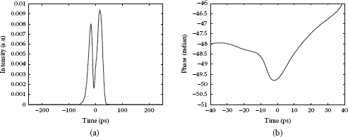
FIGURE 3.28
(a) Simulated waveform and (b) its phase profile at the 2900th round-trip showing a gray solution embedded in the building-up pulse.

FIGURE 3.29
Numerical simulated evolution of mode-locked pulse built up from noise in (a) anomalous dispersion cavity and (b) normal dispersion cavity at the same phase of modulation curve.

FIGURE 3.30
(a) Numerical simulated evolution of the signal circulating in the cavity, (b) the time trace of the output over 5000 round-trips, (c) the spectrum, and (d) the time trace averaged over the last 500 round-trips when the modulation frequency is detuned by 6 kHz.

When the detuning is small enough, the cavity remains in the mode-locked state as in asynchronous mode locking. However, the mode-locked pulse can experience a variation of temporal position induced by the frequency shift and the dispersion of the cavity. Figure 3.32 shows the behavior of the mode-locked pulse when the modulation frequency is detuned by 0.25 kHz. The contour plot in Figure 3.32b indicates that the pulse still can overcome the detuning problem to stabilize in the cavity.

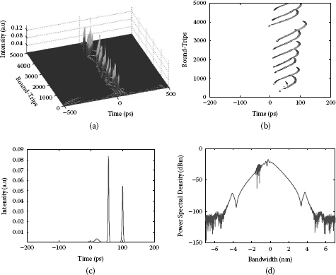
FIGURE 3.31
(a) Numerical simulated evolution of the signal circulating in the cavity, (b) contour plot view of the evolution, (c) the time trace of the output over 5000 round-trips, (d) the spectrum averaged over last 500 round-trips when the modulation frequency is detuned by 1 kHz with a higher gain factor g₀ = 0.315 m^–1 and P_sat = 8 dBm.

FIGURE 3.32
(a) Numerical simulated evolution of the mode-locked pulse circulating in the cavity. (b) Contour plot view of the evolution when the modulation frequency is detuned by 250 Hz.

3.9 Concluding Remarks

In this chapter, the fundamentals of optical pulse propagation and mode-locking mechanisms have been reviewed. In order to obtain a stable pulse train from active mode locking, some conditions have been summarized and explained. In an active mode-locked fiber laser with sufficiently high gain, the SPM effect becomes significant for pulse compression inside the anomalous dispersion average cavity to generate solitons.

Active mode-locked fiber ring lasers using the EO phase modulator have been experimentally demonstrated for the generation of a sequence of short pulses. The obtained results also indicate that the FM mode-locked fiber laser offers better performance in term of pulse width and stability than the mode-locked fiber laser using PMSL acting as an amplitude modulator. The rational harmonic mode locking has been achieved by the enhancement of higher-order harmonics in the electrical driving signal applied to the optical modulator. Moreover, the detuning effect in the fiber laser has been characterized through the time traces, optical spectrum, and RF spectrum analysis. All obtained results indicated complex behaviors in the transition regime in which the hybrid passive-active mode locking can be achieved to generate solutions of narrow pulse width.

Furthermore, a numerical model of the FM mode-locked fiber ring laser was also developed to investigate the physical processes occurring inside the fiber cavity. The formation of mode-locked pulses in various conditions of the cavity has been numerically studied to demonstrate that indeed, short pulses generated from the FM mode-locked fiber laser system are chirped solitons. The model has also been used to reproduce all possible operations of the FM mode-locked fiber laser including the detuning effect in the experiment to demonstrate the validity of the model, which would be referred to in the next chapters.

References

1. G. P. Agrawal, Nonlinear Fiber Optics, 3rd. ed. Academic Press, San Diego, 2001.

2. G. P. Agrawal, Applications of Nonlinear Fiber Optics, Academic Press, San Diego, CA, 2001.

3. G. P. Agrawal, Optical Pulse Propagation in Doped Fiber Amplifiers, Phys. Rev. A, 44, 7493, 1991.

4. S. C. Mancas and S. R. Choudhury, The Complex Cubic-Quintic Ginzburg-Landau Equation: Hopf Bifurcations Yielding Traveling Waves, Math. Comput. Simul., 74, 281–291, 2007.

5. N. Akhmediev and A. Ankiewicz, Eds., Dissipative Solitons (Lecture Notes in Physics 661). Springer, Berlin, 2005.

6. H. A. Haus et al., Structures for Additive Pulse Mode Locking, J. Opt. Soc. Am. B, 8, 2068–2076, 1991.

7. C. Menyuk, Nonlinear Pulse Propagation in Birefringent Optical Fibers, IEEE J. Quantum Electron., 23, 174–176, 1987.

8. D. Y. Tang et al., Subsideband Generation and Modulational Instability Lasing in a Fiber Soliton Laser, J. Opt. Soc. Am. B, 18, 1443–1450, 2001.

9. K. M. Spaulding et al., Nonlinear Dynamics of Mode-Locking Optical Fiber Ring Lasers, J. Opt. Soc. Am. B, 19, 1045–1054, 2002.

10. V. E. Zakharov and A. B. Shabat, Exact Theory of Two-Dimensional Self-Focusing and One-Dimensional Self-Modulation of Waves in Nonlinear Media, Soviet Physics-JETP, 34, 669, 1972.

11. Y. S. Kivshar and B. Luther-Davies, Dark Optical Solitons: Physics and Applications, Phys, Rep., 298, 81–197, 1998.

12. L. N. Binh, Photonic Signal Processing: Techniques and Applications, CRC Press, Boca Raton, FL, 2008.

13. H. Haus, A Theory of Forced Mode Locking, IEEE J. Quantum Electron., 11, 323–330, 1975.

14. M. Zirngibl et al., 1.2 ps Pulses from Passively Mode-Locked Laser Diode Pumped Er-Doped Fibre Ring Laser, Electron. Lett., 27, 1734–1735, 1991.

15. D. Abraham et al., Transient Dynamics in a Self-Starting Passively Mode-Locked Fiber-Based Soliton Laser, Appl. Phys. Lett., 63, 2857–2859, 1993.

16. B. C. Collings et al., Stable Multigigahertz Pulse-Train Formation in a Short-Cavity Passively Harmonic Mode-Locked Erbium/Ytterbium Fiber Laser, Opt. Lett., 23, 123–125, 1998.

17. N. J. Doran and D. Wood, Nonlinear-Optical Loop Mirror, Opt. Lett., 13, 56–58, 1988.

18. M. E. Fermann et al., Nonlinear Amplifying Loop Mirror, Opt. Lett., 15, 75754, 1990.

19. I. N. Duling, III, Subpicosecond All-Fibre Erbium Laser, Electron. Lett., 27, 544–545, 1991.

20. M. Nakazawa et al., Low Threshold, 290 fs Erbium-Doped Fiber Laser with a Nonlinear Amplifying Loop Mirror Pumped by InGaAsP Laser Diodes, Appl. Phys. Lett., 59, 2073–2075, 1991.

21. K. Tamura et al., 77-fs Pulse Generation from a Stretched-Pulse Mode-Locked All-Fiber Ring Laser, Opt. Lett., 18, 1080–1082, 1993.

22. K. Tamura et al., Technique for Obtaining High-Energy Ultrashort Pulses from an Additive-Pulse Mode-Locked Erbium-Doped Fiber Ring laser, Opt. Lett., 19, 46–48, 1994.

23. G. Lenz et al., All-Solid-State Femtosecond Source at 1.55 µm, Opt. Lett., 20, 1289–1291, 1995.

24. D. Y. Tang and L. M. Zhao, Generation of 47-fs Pulses Directly from an Erbium-Doped Fiber Laser, Opt. Lett., 32, 41–43, 2007.

25. H. A. Haus, Mode-Locking of Lasers, IEEE J. Selected Topics in Quantum Electron., 6, 1173–1185, 2000.

26. O. E. Martinez et al., Theory of Passively Mode-Locked Lasers Including Self-Phase Modulation and Group-Velocity Dispersion, Opt. Lett., 9, 156–158, 1984.

27. S. M. J. Kelly, Characteristic Sideband Instability of Periodically Amplified Average Soliton, Electron. Lett., 28, 806–807, 1992.

28. M. L. Dennis and I. N. Duling, III, Experimental Study of Sideband Generation in Femtosecond Fiber Lasers, IEEE J. Quantum Electron., 30, 1469–1477, 1994.

29. D. Kuizenga and A. Siegman, FM and AM Mode Locking of the Homogeneous Laser—Part I: Theory, IEEE J. Quantum Electron., 6, 694–708, 1970.

30. H. Sotobayashi and K. Kikuchi, Design Theory of Ultra-Short Pulse Generation from Actively Mode-Locked Fiber Lasers, IEICE Trans. Electron., E81-C, 201–207, 1998.

31. D. J. Jones et al., Subpicosecond Solitons in an Actively Mode-Locked Fiber Laser, Opt. Lett., 21, 1818–1820, 1996.

32. H. A. Haus and A. Mecozzi, Long-Term Storage of a Bit Stream of Solitons, Opt. Lett., 17, 1500–1502, 1992.

33. H. A. Haus and A. Mecozzi, Noise of Mode-Locked Lasers, IEEE J. Quantum Electron., 29, 983–996, 1993.

34. F. X. Kärtner et al., Solitary-Pulse Stabilization and Shortening in Actively Mode-Locked Lasers, J. Opt. Soc. Am. B, 12, 486–496, 1995.

35. K. Tamura and M. Nakazawa, Pulse Energy Equalization in Harmonically FM Mode-Locked Lasers with Slow Gain, Opt. Lett., 21, 1930–1932, 1996.

36. H. A. Haus et al., Theory of Soliton Stability in Asynchronous Modelocking, J. Lightwave Technol., 14, 62627, 1996.

37. M. Nakazawa et al., Supermode Noise Suppression in a Harmonically Modelocked Fibre Laser by Selfphase Modulation and spe, Electron. Lett., 32, 461, 1996.

38. N. G. Usechak et al., FM Mode-Locked Fiber Lasers Operating in the Autosoliton Regime, IEEE J. Quantum Electron., 41, 753–761, 2005.

39. C. R. Doerr et al., Asynchronous Soliton Mode Locking, Opt. Lett., 19, 1958–1960, 1994.

40. S. Longhi and P. Laporta, Floquet Theory of Intracavity Laser Frequency Modulation, Phys. Rev. A, 60, 4016, 1999.

41. S. Yang et al., Experimental Study on Relaxation Oscillation in a Detuned FM Harmonic Mode-Locked Er-Doped Fiber Laser, Opt. Commun., 245, 371–376, 2005.

42. S. Yang and X. Bao, Experimental Observation of Excess Noise in a Detuned Phase-Modulation Harmonic Mode-Locking Laser, Phys. Rev. A, 74, 033805, 2006.

43. Z. Ahmed and N. Onodera, High Repetition Rate Optical Pulse Generation by Frequency Multiplication in Actively Modelocked fib, Electron. Lett., 32, 455, 1996.

44. M.-Y. Jeon et al., Pulse-Amplitude-Equalized Output from a Rational Harmonic Mode-Locked Fiber Laser, Opt. Lett., 23, 855–857, 1998.

45. C. G. Lee et al., Pulse-Amplitude Equalization in a Rational Harmonic Mode-Locked Semiconductor Ring Laser Using Optical Feedback, Opt. Commun., 209, 417–425, 2002.

46. Y. Kim et al., Pulse-Amplitude Equalization in a Rational Harmonic Mode-Locked Semiconductor Fiber Ring Laser Using a Dual-Drive Mach-Zehnder Modulator, Opt. Express, 12, 907–915, 2004.

47. G. Zhu and N. K. Dutta, Eighth-Order Rational Harmonic Mode-Locked Fiber Laser with Amplitude-Equalized Output Operating at 80 Gbits/s, Opt. Lett., 30 (17), 2212–2214, 2005.

48. F. Xinhuan et al., Pulse-Amplitude Equalization in a Rational Harmonic Mode-Locked Fiber Laser Using Nonlinear Modulation, Photonics Technol. Lett., IEEE, 16, 1813–1815, 2004.

49. Y. Shiquan and B. Xiaoyi, Rational Harmonic Mode-Locking in a Phase-Modulated Fiber Laser, Photonics Technol. Lett., IEEE, 18, 1331334, 2006.

50. M. L. Dennis et al., Inherently Bias Drift Free Amplitude Modulator, Electron. Lett., 32, 547–548, 1996.

51. M. L. Dennis and I. N. Duling, III, Polarisation-Independent Intensity Modulator Based on Lithium Niobate, Electron. Lett., 36, 1857–1858, 2000.

52. Y. Shiquan and B. Xiaoyi, Repetition-Rate-Multiplication in Actively Mode-Locking Fiber Laser by Using Phase Modulated Fiber Loop Mirror, IEEE J. Quantum Electron., 41, 1285–1292, 2005.

53. H. A. Haus et al., Additive-Pulse Modelocking in Fiber Lasers, IEEE J. Quantum Electron., 30, 200–208, 1994.

54. T. F. Carruthers et al., Active-Passive Modelocking in a Single-Polarisation Erbium Fibre Laser, Electron. Lett., 30, 1051–1053, 1994.

55. C. R. Doerr et al., Additive-Pulse Limiting, Opt. Lett., 19, 31–33, 1994.

..................Content has been hidden....................

You can't read the all page of ebook, please click here login for view all page.

Table of Contents for
3 Soliton Fiber Lasers: Le Nguyen Binh and Nguyen Duc Nhan

3

Soliton Fiber Lasers

Le Nguyen Binh

CONTENTS

3.1 Introduction

3.2 Nonlinear Schrödinger Equations

3.2.1 Nonlinear Schrödinger Equation

3.2.2 Ginzburg–Landau Equation: A Modified Nonlinear Schrödinger Equation

3.2.3 Coupled Nonlinear Schrödinger Equations

3.3 Optical Solitons

3.3.1 Temporal Solitons

3.3.2 Dissipative Solitons

3.4 Generation of Solitons in Nonlinear Optical Fiber Ring Resonators

3.4.1 Master Equations for Mode Locking

3.5 Passive Mode Locking

3.6 Active Mode Locking

3.6.1 Amplitude Modulation (AM) Mode Locking

3.6.2 Frequency Modulation (FM) Mode Locking

3.6.3 Rational Harmonic Mode Locking

3.7 Actively Frequency Modulation Mode-Locked Fiber Rings: Experiment

3.7.1 Experimental Setup

3.7.2 Results and Discussion

3.7.2.1 Soliton Generation

3.7.2.2 Detuning Effect and Relaxation Oscillation

3.7.2.3 Rational Harmonic Mode Locking

3.8 Simulation of Active Frequency Modulation Mode-Locked Fiber Laser

3.8.1 Numerical Simulation Model

3.8.2 Results and Discussion

3.8.2.1 Mode-Locked Pulse Formation

3.8.2.2 Detuning Operation

3.9 Concluding Remarks

References

Table of Contents for 3 Soliton Fiber Lasers: Le Nguyen Binh and Nguyen Duc Nhan

Create new playlist

Sign In

Sign Up

3

Soliton Fiber Lasers

Le Nguyen Binh

CONTENTS

3.1 Introduction

3.2 Nonlinear Schrödinger Equations

3.2.1 Nonlinear Schrödinger Equation

3.2.2 Ginzburg–Landau Equation: A Modified Nonlinear Schrödinger Equation

3.2.3 Coupled Nonlinear Schrödinger Equations

3.3 Optical Solitons

3.3.1 Temporal Solitons

3.3.2 Dissipative Solitons

3.4 Generation of Solitons in Nonlinear Optical Fiber Ring Resonators

3.4.1 Master Equations for Mode Locking

3.5 Passive Mode Locking

3.6 Active Mode Locking

3.6.1 Amplitude Modulation (AM) Mode Locking

3.6.2 Frequency Modulation (FM) Mode Locking

3.6.3 Rational Harmonic Mode Locking

3.7 Actively Frequency Modulation Mode-Locked Fiber Rings: Experiment

3.7.1 Experimental Setup

3.7.2 Results and Discussion

3.7.2.1 Soliton Generation

3.7.2.2 Detuning Effect and Relaxation Oscillation

3.7.2.3 Rational Harmonic Mode Locking

3.8 Simulation of Active Frequency Modulation Mode-Locked Fiber Laser

3.8.1 Numerical Simulation Model

3.8.2 Results and Discussion

3.8.2.1 Mode-Locked Pulse Formation

3.8.2.2 Detuning Operation

3.9 Concluding Remarks

References

Table of Contents for
3 Soliton Fiber Lasers: Le Nguyen Binh and Nguyen Duc Nhan