
To recognize optical characters, we produced data to train and to test the neural network. In this example, we considered digits from zero to nine. According to the pixel layout, two versions of each digit data were created, one to train and the other to test. Classification techniques presented in Chapter 3, Handling Perceptrons, and Chapter 6, Classifying Disease Diagnosis will be used here.
Numbers from zero and nine were represented by matrices in the following figure. Black pixels are typified by the value one and white pixels by the value zero. All pixel values between zero and one are on grayscale. The first dataset is to train the neural network, and the second one is for testing. It's possible to detect some random noise in the test dataset. We performed this procedure deliberately to verify the generalization.

Training dataset

Test dataset
Each matrix row was merged into vectors (Dtrain / Dtest) to form a pattern that will be used to train and test the neural network. Therefore, the input layer of the neural network will be composed of 26 neurons. The following tables show this data:
|
Training Input Dataset |
|---|
|
Dtrain(0) = [1,0,1,1,1,0,1,0,0,0,1,1,0,0,0,1,1,0,0,0,1,0,1,1,1,0] Dtrain(1) = [1,0,0,1,0,0,0,1,1,0,0,1,0,1,0,0,0,0,1,0,0,0,0,1,0,0] Dtrain(2) = [1,1,1,1,1,1,0,0,0,0,1,1,1,1,1,1,1,0,0,0,0,1,1,1,1,1] Dtrain(3) = [1,1,1,1,1,1,0,0,0,0,1,0,1,1,1,1,0,0,0,0,1,1,1,1,1,1] Dtrain(4) = [1,1,0,0,0,1,1,0,0,0,1,1,1,1,1,1,0,0,0,0,1,0,0,0,0,1] Dtrain(5) = [1,0,1,1,1,0,0,1,0,0,0,0,1,1,1,0,0,0,0,1,0,0,1,1,1,0] Dtrain(6) = [1,0,1,1,1,0,1,0,0,0,0,1,1,1,1,1,1,0,0,0,1,0,1,1,1,0] Dtrain(7) = [1,0,1,1,1,1,0,0,0,0,1,0,0,0,0,1,0,0,0,0,1,0,0,0,0,1] Dtrain(8) = [1,0,1,1,1,0,1,0,0,0,1,1,1,1,1,1,1,0,0,0,1,0,1,1,1,0] Dtrain(9) = [1,0,1,1,1,0,1,0,0,0,1,0,1,1,1,1,0,0,0,0,1,0,0,0,0,1] |
|
Test Input Dataset |
|---|
|
Dtest(0) = [1,0.5,1,1,1,0.5,1,0,0,0,1,1,0,0,0,1,1,0,0,0,1,0.5,1,1,1,0.5] Dtest(1) = [1,0,0,1,0,0,0,0.5,1,0,0,0.25,0,1,0,0,0,0,1,0,0,0,0,1,0,0] Dtest(2) = [1,1,1,1,1,1,0.2,0,0,0,1,1,1,1,1,1,1,0,0,0,0.2,1,1,1,1,1] Dtest(3) = [1,0.5,1,1,1,1,0,0,0,0,1,0,0,1,1,1,0,0,0,0,1,0.5,1,1,1,1] Dtest(4) = [1,0.5,0,0.5,0,1,1,0,0,0,1,1,1,1,1,0.5,0,0,0,0,1,0.5,0,0,0,1] Dtest(5) = [1,0,1,1,0.5,0,0,1,0,0,0,0,1,1,1,0,0,0,0,0.5,0.5,0,0.5,1,1,0] Dtest(6) = [1,0,1,1,0.1,0,1,0,0,0,0,1,1,1,1,1,0.5,0,0,0,0.5,0,1,1,1,0] Dtest(7) = [1,0,1,1,0.5,0.5,0,0,0,1,0,0,0,1,0,0,0,1,0,0,0,0.5,0,0,0,0.5] Dtest(8) = [1,0,0.9,1,0.9,0,0.7,0,0,0,0.8,1,1,0.5,1,1,0.8,0,0,0,0.7,0,0.8,1,0.8,0] Dtest(9) = [1,0,1,1,0.5,0,0.5,0,0,0,1,0,0.5,1,1,1,0,0,0,0,1,0,0,0,0,0.5] |
The output dataset was represented by 10 patterns. Each one has a more expressive value (1) and the rest are zero. Therefore, the output layer of the neural network will have 10 neurons, as shown in the following table:
|
Output Dataset |
|---|
|
Out(0) = [0,0,0,0,0,0,0,0,0,1] Out(1) = [1,0,0,0,0,0,0,0,0,0] Out(2) = [0,1,0,0,0,0,0,0,0,0] Out(3) = [0,0,1,0,0,0,0,0,0,0] Out(4) = [0,0,0,1,0,0,0,0,0,0] Out(5) = [0,0,0,0,1,0,0,0,0,0] Out(6) = [0,0,0,0,0,1,0,0,0,0] Out(7) = [0,0,0,0,0,0,1,0,0,0] Out(8) = [0,0,0,0,0,0,0,1,0,0] Out(9) = [0,0,0,0,0,0,0,0,1,0] |
So, in this application, our neural network shall have 25 inputs and 10 outputs, so we varied the number of hidden neurons. We created a class called Digit in the package ocr to handle this application. The neural network architecture was designed with the following parameters and represented by the following figure:
- Neural network type: MLP
- Training algorithm: Backpropagation
- Number of hidden layers: 1
- Number of neurons in the hidden layer: 18
- Number of epochs: 6000

Now, as has been done in other case studies presented previously, let's find the best neural network topology training several nets. The strategy to do that is summarized in the following table:
|
Experiment |
Learning Rate |
Activation Functions |
|---|---|---|
|
1 |
0.5 |
Hidden layer: SIGLOG |
|
Output layer: SIGLOG | ||
|
2 |
0.7 |
Hidden layer: SIGLOG |
|
Output layer: SIGLOG | ||
|
3 |
0.9 |
Hidden layer: SIGLOG |
|
Output layer: SIGLOG | ||
|
4 |
0.5 |
Hidden layer: SIGLOG |
|
Output layer: HYPERTAN | ||
|
5 |
0.7 |
Hidden layer: SIGLOG |
|
Output layer: HYPERTAN | ||
|
6 |
0.9 |
Hidden layer: SIGLOG |
|
Output layer: HYPERTAN | ||
|
7 |
0.5 |
Hidden layer: SIGLOG |
|
Output layer: LINEAR | ||
|
8 |
0.7 |
Hidden layer: SIGLOG |
|
Output layer: LINEAR | ||
|
9 |
0.9 |
Hidden layer: SIGLOG |
|
Output layer: LINEAR |
The following piece of code of the Digit class defines how to create a neural network to read from digit data:
  Data ocrDataInput  = new Data("data\ocr", "ocr_traning_inputs.csv");
  Data ocrDataOutput = new Data("data\ocr", "ocr_traning_outputs.csv");
  //read the data points coded in a csv file
  Data ocrDataInputTestRNA  = new Data("data\ocr", "ocr_test_inputs.csv");
  Data ocrDataOutputTestRNA = new Data("data\ocr", "ocr_test_outputs.csv");

  // convert these files into matrices
  double[][] matrixInput  = ocrDataInput.rawData2Matrix( ocrDataInput );
  double[][] matrixOutput = ocrDataOutput.rawData2Matrix( ocrDataOutput );

  //creates a neural network
  NeuralNet n1 = new NeuralNet();
  //25 inputs, 1 hidden layer, 18 hidden neurons and 10 outputs
      n1 = n1.initNet(25, 1, 18, 10);

      n1.setTrainSet( matrixInput );
      n1.setRealMatrixOutputSet( matrixOutput );

//set the training parameters
      n1.setMaxEpochs(6000);
      n1.setTargetError(0.00001);
      n1.setLearningRate( 0.7 );
      n1.setTrainType(TrainingTypesENUM.BACKPROPAGATION);
      n1.setActivationFnc(ActivationFncENUM.SIGLOG);
n1.setActivationFncOutputLayer(ActivationFncENUM.SIGLOG);After running each experiment using the Digit class and saving the MSE values (according to the following table), we can observe that experiments 2 and 4 have the lowest MSE values. The differences between these two experiments are the learning rate and the activation function used in the output layer.
|
Experiment |
MSE Training Rate |
|---|---|
|
1 |
0.03007294436333284 |
|
2 |
0.02004457991277001 |
|
3 |
0.03002653392502009 |
|
4 |
0.00119817123282438 |
|
5 |
0.06351562546547934 |
|
6 |
0.23755154264016012 |
|
7 |
0.19155179860965179 |
|
8 |
1.73485602025775039 |
|
9 |
44.1822391373913359 |
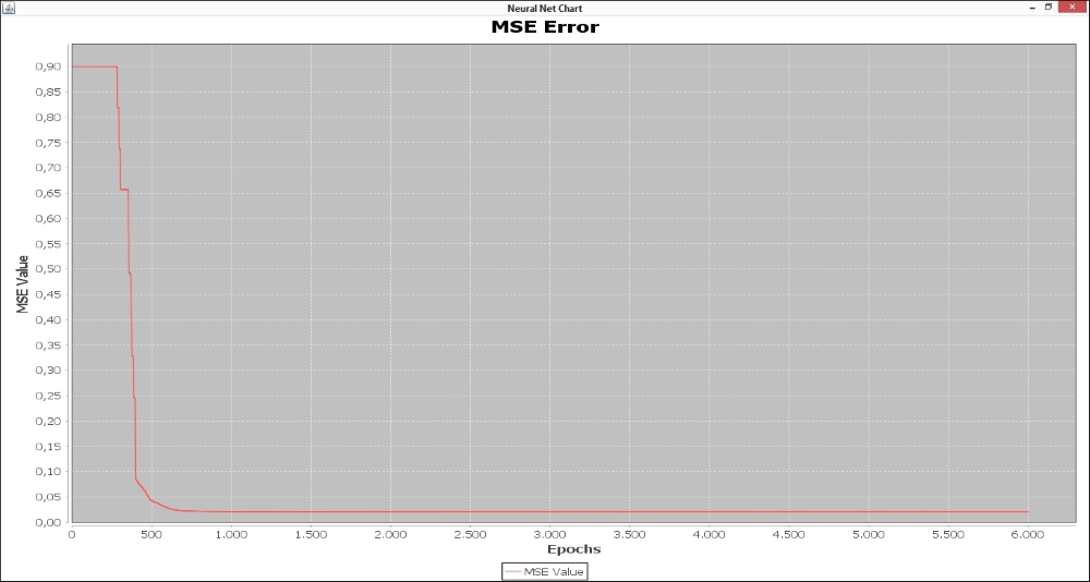
The MSE evolution over the training epochs is plotted in the following figures. It is interesting to note that the curve of experiment 2 stabilizes near the 750th epoch, as shown in the following figure:
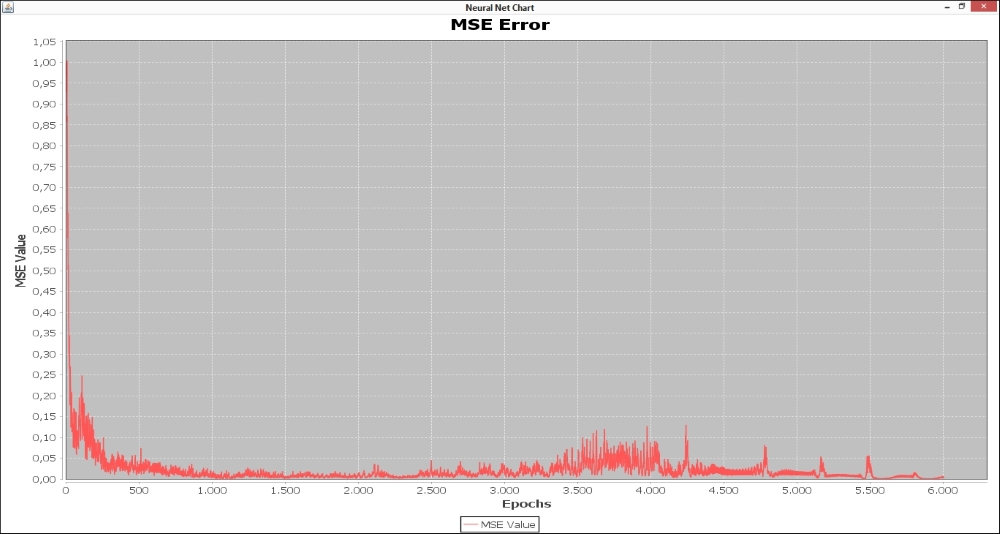
However, the curve of experiment 4 keeps varying until the 6000th epoch, as shown in the following figure:
We have already explained that only the MSE value should not be considered to attest to neural net quality. Accordingly, the test dataset was used to verify the neural network generalization capacity. A comparison between the real output with noise and the neural net estimated output of experiments 2 and 4 is depicted in the following table. It is possible to conclude that the neural network weights obtained by experiment 4 are able to better recognize digits from zero to nine even if the images present pixels noisier than those obtained by experiment 2. While experiment 2 erroneously classified three patterns, experiment 4 classified all patterns correctly.
|
Output Comparison | |
|---|---|
|
Real Output (Test Dataset) |
Digit |
|
0.00  0.00  0.00  0.00  0.00  0.00  0.00  0.00  0.00  1.00
1.00  0.00  0.00  0.00  0.00  0.00  0.00  0.00  0.00  0.00
0.00  1.00  0.00  0.00  0.00  0.00  0.00  0.00  0.00  0.00
0.00  0.00  1.00  0.00  0.00  0.00  0.00  0.00  0.00  0.00
0.00  0.00  0.00  1.00  0.00  0.00  0.00  0.00  0.00  0.00
0.00  0.00  0.00  0.00  1.00  0.00  0.00  0.00  0.00  0.00
0.00  0.00  0.00  0.00  0.00  1.00  0.00  0.00  0.00  0.00
0.00  0.00  0.00  0.00  0.00  0.00  1.00  0.00  0.00  0.00
0.00  0.00  0.00  0.00  0.00  0.00  0.00  1.00  0.00  0.00
0.00  0.00  0.00  0.00  0.00  0.00  0.00  0.00  1.00  0.00
|
0 1 2 3 4 5 6 7 8 9 |
|
Estimated Output (Test Dataset) – Experiment 2 |
Digit |
|
0.00  0.00  0.00  0.00  0.00  0.01  0.02  0.00  0.00  0.97
0.97  0.00  0.00  0.00  0.03  0.00  0.00  0.00  0.00  0.00
0.00  0.00  0.00  0.02  0.00  0.00  0.00  0.01  0.00  0.00
0.00  0.00  0.00  0.02  0.00  0.00  0.20  0.00  0.00  0.00
0.00  0.00  0.00  0.96  0.00  0.00  0.00  0.02  0.00  0.00
0.01  0.00  0.00  0.00  0.98  0.01  0.00  0.00  0.00  0.00
0.01  0.00  0.00  0.00  0.00  0.56  0.00  0.07  0.00  0.00
0.00  0.00  0.00  0.00  0.66  0.00  0.14  0.00  0.00  0.00
0.00  0.00  0.00  0.00  0.00  0.03  0.00  0.93  0.00  0.01
0.00  0.00  0.00  0.00  0.01  0.00  0.00  0.01  0.96  0.00
|
0 (OK) 1 (OK) 4 (ERR) 7 (ERR) 4 (OK) 5 (OK) 6 (OK) 5 (ERR) 8 (OK) 9 (OK) |
|
Estimated Output (Test Dataset) – Experiment 4 |
Digit |
|
 0.00  0.16  0.09  0.06  0.06   0.01  0.11 -0.27 -0.09  0.97
 1.00  0.00  0.09  0.13  0.21 -0.22  0.42  0.19  0.34  0.14
 0.00  0.99  0.04  0.05  0.07  0.10  0.14  0.18  0.22  0.25
 0.01  0.03  0.81  0.06  0.09   0.03  0.74 -0.03 -0.03 -0.12
 0.02 -0.11 -0.10  0.94  0.08  0.08  0.11  0.85  0.09  0.06
 0.02 -0.01  0.10  0.06  1.00  0.11  0.10  0.11  0.10  0.06
-0.00 -0.07 -0.05  0.22  0.09   1.00  0.20  0.11  0.26  0.20
 0.51 -0.05  0.25  0.09  0.96  0.22  0.99  0.25  0.34  0.34
 0.00  0.04  0.04  0.04  0.05  0.06  0.05  0.98  0.03  0.07
 0.00  0.01  0.05  0.01  0.02  0.00  0.04  0.03  1.00  0.02
|
0 (OK) 1 (OK) 2 (OK) 3 (OK) 4 (OK) 5 (OK) 6 (OK) 7 (OK) 8 (OK) 9 (OK) |