
So far, we have theoretically defined the learning process and how it is carried out. However, in practice, we must dive a little bit deeper into the mathematical logic, the learning algorithm itself. A learning algorithm is a procedure that drives the learning process of neural networks and is strongly determined by the neural network architecture. From the mathematical point of view, one wishes to find the optimal weights W that can drive the cost function C(X,[Y]) to the lowest possible value.
In general, this process is carried out in the fashion presented in the following flowchart:

Just like any program that we wish to write, we should have defined our goal, so in here, we are talking about a neural network to learn some knowledge. We should present this knowledge (or environment) to the ANN and check its response, which naturally will make no sense. The network response is then compared to the expected result, and this is fed to a cost function C. This cost function will determine how the weights W can be updated. The learning algorithm then computes the ΔW term, which means the variation of the values of the weights to be added. The weights are updated as in the equation.
Where k refers to the kth iteration and W(k) refers to the neural weights at the kth iteration, and subsequently, k + 1 refers to the next iteration.
As the learning process is run, the neural network must give results closer and closer to the expectation, until finally, it reaches the acceptation criteria. The learning process is then considered to be finished.
Well, we might ask now whether the neural network has already learned from the data, but how can we attest it has effectively learnt the data? The answer is just like in the exams that students are subjected to; we need to check the network response after training. But wait! Do you think it is likely that a teacher would put in an exam the same questions he/she has presented in the classes? There is no sense in evaluating somebody's learning with examples that are already known or a suspecting teacher would conclude the student might have memorized the content, instead of having learnt it.
Okay, let's now explain this part. What we are talking about here is testing. The learning process that we have covered is called training. After training a neural network, we should test it whether it has really learnt. For testing, we must present to the neural network another fraction of data from the same environment that it has learnt from. This is necessary because, just like the student, the neural network could respond properly with only the data points that it had been exposed to; this is called overtraining. To check whether the neural network has not passed on overtraining, we must check its response to other data points.
The following figure illustrates the overtraining problem. Imagine that our network is designed to approximate some function f(x) whose definition is unknown. The neural network was fed with some data from that function and produced the following result shown in the figure on the left. However, when expanding to a wider domain, we note that the neural response does not follow the data.
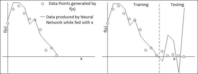
In this case, we see that the neural network failed to learn the whole environment (the function f(x)). This happens because of a number of reasons:
- The neural network didn't receive enough information from the environment
- The data from the environment is nondeterministic
- The training and testing datasets are poorly defined
- The neural network has learnt a lot from the training data and forgets about the testing data
In this book, we will cover this process to prevent this and other issues that may arise during training.
The learning process may be, and is recommended to be, controlled. One important parameter is the learning rate, often represented by the Greek letter η. This parameter dictates how strongly the neural weights would vary in the weights' hyperspace. Let's imagine a simple neural network with two inputs and one neuron, therefore one output. So, we've got two weights w1 and w2. Now suppose that we want to train this network and imagine whether we could evaluate the error for each pair of weights. Suppose that we found a surface like the one in the following figure:

The learning rate is responsible for regulating how far the weights are going to move on the surface. This may speed up the learning process but can also lead to a set of weights worse than the previous one.
Another important parameter is the condition for stopping. Usually, the training stops when the general mean error is reached, but there are cases in which the network fails to learn and there is little or no change in the weights' values. In the latter case, the maximum number of iterations, or epochs, is the condition for stopping.
This is extremely important for the success of the training in the supervised learning. Let's suppose that we present for the network a set of N records containing pairs of X and T variables, whereas X are the input-independent values and T are the target values dependent on X. Let's consider the neural network as a mathematical function ANN() that produces Y on the output when being fed with the X values.
For each x value given to the ANN, it will produce a y value that when compared to the t value gives an error e.
However, this is a mere individual error measurement per data point. We should take into account a general measurement, covering all the N data pairs because we want the network to learn all the data points and the same weights must be able to produce the data covering the entire training set. That's the role of the cost function C.

Where X are the inputs, T are the target outputs, W are the weights, x[i] is the input at the ith instant, and t[i] is the target output for the ith instant. The result of this function is an overall measurement of the error between the target outputs and the neural outputs, and this should be minimized.