
This network architecture was created by the Finnish professor Teuvo Kohonen at the beginning of the 80s. It consists of one single-layer neural network capable of providing a "visualization" of the data in one or two dimensions.
Tip
Theoretically, a Kohonen network would be able to provide a 3D (or even a higher-dimensional) representation of the data; however, in printed material, such as this book, it is not possible to show 3D charts without overlapping some data. Thus, in this book, we are going to deal only with 1D and 2D Kohonen networks.
The major difference between the Kohonen SOMs and the traditional single-layer competitive neural networks is the concept of neighborhood neurons. While in a neural network, usually, there is no importance of the order in which the neurons are positioned in the output, in an SOM, the neighboring neurons play a relevant role during the learning phase.
An SOM has two modes of functioning: mapping and learning. In the mapping mode, the input data is classified in the most appropriate neuron, while in the learning mode, the input data helps the learning algorithm to build the "map." This map can be interpreted as a lower-dimensional representation from a certain dataset.
In this chapter, we are going to present two types of SOMs: 1D and 2D SOMs.
This architecture is similar to the network presented in the last section: competitive learning, with the addition of the neighborhood amongst the output neurons.
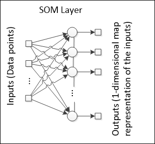
Note that every neuron on the output layer has two neighbors. Similarly, the neuron that fires the greatest value updates its weights, but in an SOM, the neighboring neurons also update their weights at a relatively slow rate.
The effect of the neighborhood extends the activation area to a wider area of the map, provided that all the output neurons observe an organization, a path in the 1D case. The neighborhood function also allows for a better exploration of the properties of the input space, since it forces the neural network to maintain the connections between neurons, therefore resulting in more information in addition to only the clusters that are formed.
In a plot of the input data points with the neural weights, we can see the path formed by the neurons.

In the chart presented here, for the sake of simplicity, we plotted only the output weights to demonstrate how the map is designed in a (in this case) 2D space. After training over many iterations, the neural network converges to the final shape that represents all data points. Provided this structure, a certain set of data may cause the Kohonen network to design another shape in the space. This is a good example of dimensionality reduction, since a multidimensional dataset when presented to the SOM is able to produce a single line (in the 1D SOM) that "summarizes" the entire dataset.
This is the architecture that is most frequently used to demonstrate the power of a Kohonen neural network visually. The output layer is a matrix containing N x N neurons, interconnected like a grid:
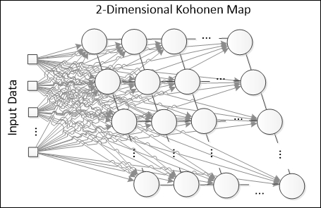
In 2D SOMs, every neuron now will have up to four neighbors, although in some representations, the diagonal neurons may also be considered, thus resulting in up to eight neighbors. Basically, the working principle of 2D SOMs is the same. Let's see an example of how a 3 x 3 SOM plot looks in a 2D chart (considering two input variables):

First, the untrained Kohonen network shows a shape that is very strange and screwed up. The shape of the weights will depend solely on the input data that are going to be fed to the SOM. Let's see an example of how the map starts to organize itself.
- Suppose that we have the dense dataset shown in the following plot:

- Upon the application of the SOM, the 2D shape gradually changes, until the network achieve its final configuration:

The final shape of a 2-D SOM may not always be a perfect square; instead, it will resemble a shape that could be drawn from the dataset. The neighborhood function is an important component in the learning process because it approximates the neighboring neurons in the plot, and the structure moves to a configuration that is more "organized."
An SOM aims at classifying the input data by clustering data points that trigger the same response on the output. Initially, the untrained network will produce random outputs, but as more examples are presented, the neural network identifies which neurons are more often activated, and then, their "position" in the SOM output space is changed. This algorithm is based on competitive learning, which means that a winner neuron (also known as Best Matching Unit, BMU) will update its weights and its neighboring weights.
The following flowchart illustrates the learning process of an SOM network:

The learning slightly resembles that of the algorithms addressed in Chapter 2, How Neural Networks Learn and Chapter 3, Handling Perceptrons. The three major differences are the determination of the BMU with the distance, the weight update rule, and the absence of an error measure. The distance implies that nearer points should produce similar outputs; thus, here, the criteria to determine the BMU is the neuron that presents a lower distance to some data point. This Euclidean distance is usually used, and in this book, we will apply it for the sake of simplicity:
The weight update rule uses the neighborhood function Θ(i,j), which states how much a neighboring neuron i is close to neuron j. Remember that in the SOM, the BMU neuron is updated together with its neighboring neurons. The update rule is as follows:
Where α denotes the learning rate; Θ, the neighborhood function; Xk, the kth input; and Wkj, the weight connecting the kth input to the jth output. Another characteristic of this learning is that both the learning rate and the neighborhood function are dependent on the number of epochs. The neighborhood function is usually Gaussian:
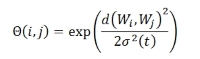
Where σ denotes the Gaussian parameter of variance, Wi and Wj represent the weights of neurons i and j, and t denotes the number of epochs.
The learning rate starts at an initial value and then decreases:
Where r represents a parameter of the learning rate.
There are many applications of SOMs, most of them in the field of clustering, data abstraction, and dimensionality reduction. However, the clustering applications are the most interesting because of the many possibilities one may apply them to. The real advantage of clustering is that there is no need to worry about the input–output relationship; rather, the problem solver can concentrate on the input data. One example of a clustering application will be explored in Chapter 7, Clustering Customer Profiles.