
In this section, we optimize two parameters in OppCast: the forwarding range FR and threshold density ρth.
10.6.1 Optimize the Forwarding Range
As mentioned in Section 10.5.1, the goal here is to minimize the expected total number of transmissions E[NT]. Stated formally, we want to find the FR
10.7 ![]()
10.8 ![]()
Algorithm 10.1 Distributed OppCast algorithm running at node u
Input: Node u receives a WM m; If u is in the IR of m, and m is a new packet If typeprevhop = forwarder and xu > xright //Enter FFD; If (xu − xright) < the local optimal boundary range (LBR) Set xD = xright + LBR, xI = xright; //the RCR Compute Δtu and run OBCF; //potential forwarder If u becomes a forwarder Useto compute the new local optimal boundary range;
Set xleft = xright, xright = xu; Increase the one-hop zone index by 1 and broadcast m. If xleft < xu < xright //potential makeup If typeprevhop = forwarder //Initialize MFR Makeup node level= 0; sub-zone index μ = 0;
If, then exit;
Set the visited node location list VL:{x0 = xleft, x1 = xright}; If typeprevhop = makeup //Enter MFR; xprev ← last element in VL; If xu > xprev xleft = xprev, μ = 2μ + 1;// boundary of current sub-zone; Else, xright = xprev, μ = 2μ; If, then exit;
xW = (xleft + xright)/2; If
         If xu ≥ xW
            xD = xW, xI = xright; //The RCR;
         Else if xu < xW
            xD = xW, xI = xleft; //The RCR;
         Calculate Δtu and run OBCF;
The optimization is targeted at the well connected case (vehicle density is larger than ρth), whereas it is straightforward to show that under the strategies of the FFD and MFR phases, the constraint is satisfied with high probability.
Thus, we first compute the expected number of transmissions (E[NT]), based on which the optimal FR is derived. We introduce the centralized solution to find the optimal FR and then propose a distributed, locally optimized version. The centralized solution takes as input the average vehicle density ρ of IR, and approximates the E[NT]. Since E[NT] has no closed form expression, the optimal FR that minimizes E[NT] is sought out by sampling and searching.
Let us consider a one-dimensional VANET where the IR length ![]() is sufficiently large. Assume there are no redundant transmissions and no packet collisions. Further, we assume there are enough relay candidates so that the PRP requirement can always be satisfied. Finally, the Rayleigh fading model is used for pairwise PRP function:
is sufficiently large. Assume there are no redundant transmissions and no packet collisions. Further, we assume there are enough relay candidates so that the PRP requirement can always be satisfied. Finally, the Rayleigh fading model is used for pairwise PRP function: ![]() , where Prxth is the reception threshold power, Pref is the reference receive power at distance 1 m by free space propagation model.
, where Prxth is the reception threshold power, Pref is the reference receive power at distance 1 m by free space propagation model.
The total number of transmissions NT can be expressed as:
10.9 
10.10 
where X is the number of one-hop zones, and Mi is the number of makeups in the ith one-hop zone. Yi is the length of the ith one-hop zone, and M = M(Y) is a single-variable function of Y, while Y is related to both FR and ρ. ω is the number of retransmissions made by the ith forwarder. Since Yi are i.i.d. random variables, X is also a random variable.
Therefore, we have
10.11 ![]()
For an approximation, we neglect the dependence between X and Yi (i.e. ![]() ), then
), then
10.12 ![]()
and thus
where E[X] is the average number of one-hop zones, E[M] is the average number of makeups in each one-hop zone, E[Y] is the average one-hop zone length, E[ω] is the expected retransmission count of each forwarder.
We then approximate E[Y] and E[M] by fixing the inter space between successive vehicles to3 L = 1000/ρ.
where ![]() . From Figure 10.8, we can see that the above equation yields a good approximation to the average one-hop zone length. Similarly,
. From Figure 10.8, we can see that the above equation yields a good approximation to the average one-hop zone length. Similarly,
10.15 
where M(kL) is the number of makeups needed in an one-hop zone of length kL under the ideal case where each makeup locates in the middle of its parent's subzone.
Figure 10.8 Numerical validation of E[Y]. Reproduced by permission of © 2009 IEEE.

For each forwarder, the expected number of retransmissions to be made is:
10.16 
and E[ω] = min{E[ω]′, MAX_RETX}.
Finally, the expected total number of transmissions is obtained by Equation (10.13). E[NT] is a function of both FR and ρ; however, it has no closed form solution. Under a fixed ρ, the optimal FR that minimizes E[NT] can be obtained by searching FR from L to Rc (e.g. 500 m), by setting the sampling interval to a small enough value, e.g., 10 m.
10.6.1.1 Theoretical Insights
First, we carry out simulations to verify the above results. An idealized version of the protocol (referred to as IDEAL) is implemented in NS2, where the BACK can be reliably received by all nodes in the network. The averaged vehicle density in IR is adopted as an input in IDEAL.
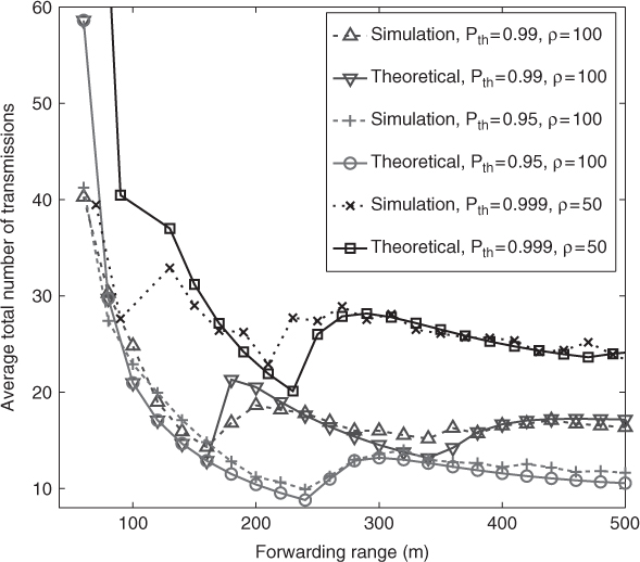
Figure 10.9 compares the theoretical value of E[NT] to the average number of transmissions in IDEAL. The theoretical values are close to the simulated values for all the vehicle densities and Pth shown, and the same for the optimal points of FR.
Figure 10.9 Numerical validation of E[NT], ![]() = 2km. Reproduced by permission of © 2009 IEEE.
= 2km. Reproduced by permission of © 2009 IEEE.
Interestingly, the optimal FR also exhibits opportunistic behavior, depending on the required PRR and vehicle density. In Figure 10.10, the optimal FR increases and decreases recurringly as the Pth increases. The reason is twofold. 1. On the one hand, using some particular “longer hops” reduces the number of transmissions. Note that the E[NT] ∼ E[Y] function has multiple local minimas4. Using a more distant minimal point not only reduces the number of hops but also contributes to the APRP of the other nodes. 2. On the other hand, the longer a hop is, the less possible it is for a WM to reach that far. The E[Y] is upper-bounded when ρ is fixed.
Figure 10.10 Optimal forwarding range, ![]() = 5km. Reproduced by permission of © 2009 IEEE.
= 5km. Reproduced by permission of © 2009 IEEE.

For example, when CR = 250 m, E[Y] is always less than 350 m. For Pth = 0.95, the first two local minimal points are E[Y] = 220 and 450, which implies the FR corresponding to the first one is optimal. Therefore, the above results indicate that when the network is well connected, the best strategy is try to use long hops opportunistically but only when it is feasible to reach that long hop statistically.
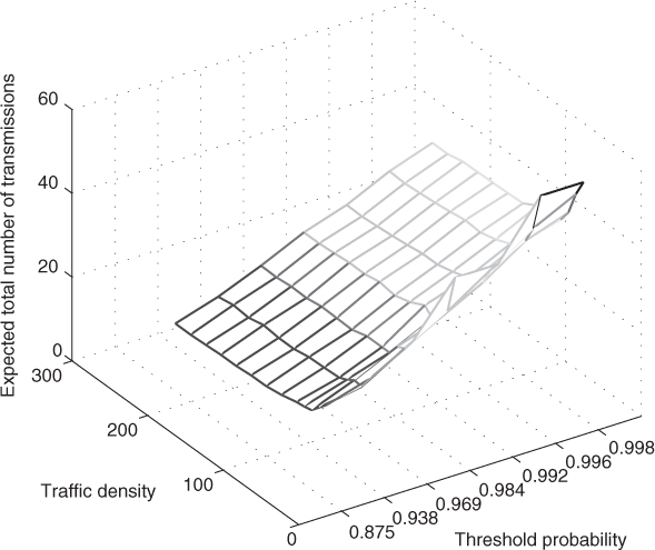
Finally, in Figure 10.11 the average total number of retransmissions increase linearly when the threshold probability increases inverse exponentially towards 1. This reveals the intrinsic tradeoff between the desired WM reception ratio and transmission count, which is a helpful result for WM broadcast applications in VANETs.
Figure 10.11 Expected total number of transmissions, ![]() = 5km. CR = 250m in all figures. © 2011 IEEE. Reprinted, with permission, from Z. Yang, M. Li and W. Lou, “CodePlay: Live Multimedia Streaming in VANETs using Symbol-Level Network Coding”, IEEE Transactions on Mobile Computing (TMC), 2011.
= 5km. CR = 250m in all figures. © 2011 IEEE. Reprinted, with permission, from Z. Yang, M. Li and W. Lou, “CodePlay: Live Multimedia Streaming in VANETs using Symbol-Level Network Coding”, IEEE Transactions on Mobile Computing (TMC), 2011.
10.6.1.2 Distributed Algorithm
In OppCast, a distributed algorithm is used to set the FR because global vehicle density information is not available. Each node calculates its own optimal FR based on the local vehicle density estimated from its direct neighbor nodes' locations. A node is considered to be a neighbor as long as a beacon is heard from it within 1 s. Each forwarder estimates its local traffic density ![]() , based on which a local optimal FR is derived and included in every rebroadcast packet, and every vehicle that receives it use the same FR included in the packet. In addition, an upper limit (for example, 1000 m) is imposed on the FR to prevent the hop delay from being too large.
, based on which a local optimal FR is derived and included in every rebroadcast packet, and every vehicle that receives it use the same FR included in the packet. In addition, an upper limit (for example, 1000 m) is imposed on the FR to prevent the hop delay from being too large.
Note that, in the OppCast extension to the sparse VANET, due to a short optimal FR at some traffic densities, while the vehicles that received the WM may all be located outside the FR, there is a small chance of forwarder shortage. To deal with this situation, we let each forwarder increase its FR by 2× after it retransmits the same packet another time, until reaching the limit.
10.6.1.3 Discussion
Our optimization is carried out using the equal inter distance vehicle distribution model (regularly distributed). However, through Figure 10.8 and Figure 10.9, it can be seen that the results are not so sensitive to the uniform vehicle distribution, which is a common mobility model adopted in most previous works. In fact, the variations in vehicle densities in the regular and uniform models are both small. In reality, some vehicles may travel in platoons; one may wonder if such mobility pattern would affect the effectiveness of optimization. Let us imagine a well-connected platoon of length 1 km; the vehicles in it can often be regarded as nearly regularly distributed. Since the distributed algorithm is based on local traffic density estimation, and the range of “locality” is really restricted to CR = 250 m (Equation (10.6)), the algorithm is expected to work well for vehicles within the platoon. Near the boundaries of the platoon, if the local density falls below ρth, the vehicle density experiences large variation; store-carry-forward will be used where the optimization does not play an important role. If the local density are larger than ρth, the variations in density are relatively small and our algorithm still applies well.
10.6.2 Optimal Threshold Density
Above a certain threshold density, the network is connected and the PRR requirement can be satisfied, but a higher threshold is unnecessary, which incurs redundant transmissions. Thus, we first calculate the probability that the VANET is connected, which means successive forwarders can be selected to propagate the WM towards the end of IR. Still using the simplified model in the above, for a given ρ, the probability that a forwarder is selected for one hop equals
10.17 
where FRopt is the optimal FR. The expected number of hops equals ![]() , where E[Y] is computed from Equation (10.14), by substituting FR with FRopt. Thus
, where E[Y] is computed from Equation (10.14), by substituting FR with FRopt. Thus
10.18 ![]()
The result is shown in Figure 10.12. It can be seen that when Pth = 0.95, the optimal ρth is between 15-20.
Figure 10.12 Probability that the VANET is connected, CR = 250m, ![]() = 5km. © 2011 IEEE. Reprinted, with permission, from Z. Yang, M. Li and W. Lou, “CodePlay: Live Multimedia Streaming in VANETs using Symbol-Level Network Coding”, IEEE Transactions on Mobile Computing (TMC), 2011.
= 5km. © 2011 IEEE. Reprinted, with permission, from Z. Yang, M. Li and W. Lou, “CodePlay: Live Multimedia Streaming in VANETs using Symbol-Level Network Coding”, IEEE Transactions on Mobile Computing (TMC), 2011.
