
In this section, we describe the components of OppCast. We begin by introducing the FFD and MFR phases from the high level, and then present the underlying OBCF MAC protocol used in relay selection for each transmission. The main notation in this chapter is summarized in Table 10.1.
Table 10.1 Summary of main notation
| RCR | Relay candidate region |
| FR | The forwarding range (length of forwarder's RCR) |
| IR | The interested region |
| PRR | Packet reception ratio |
| F | A forwarder |
| G(V, E) | The modeled graph of the VANET in IR |
| Pth | The required PRR threshold |
| d(u, v) | Distance between two nodes u and v |
| Pr(x) | Packet reception probability at a distance x |
| ξ(v) | Accumulated packet reception probability (APRP) at node v |
| E[NT] | Expected total number of transmissions |
| M |
A makeup node at the |
| Z |
A subzone of |
| W |
The middle point used to select makeup node M |
| Δtv | The backoff delay of node v for relay contention |
| ρ | Vehicle density |
© 2011 IEEE. Reprinted, with permission, from Z. Yang, M. Li and W. Lou, “CodePlay: Live Multimedia Streaming in VANETs using Symbol-Level Network Coding”, IEEE Transactions on Mobile Computing (TMC), 2011.
10.5.1 Fast-Forward Dissemination
The goal of the FFD phase is to achieve fast WM propagation by using relatively long forwarding hops. Immediately after each forwarder F rebroadcasts, all nodes within the forwarder RCR that receive the WM are candidate forwarders and participate in the contention process to become the next hop forwarder. For F, its forwarder RCR is a road segment from F towards the end of IR, whose length is called the forwarding range (FR). The priority of the candidate forwarders increases with the hop progress (their distance to F), in order to maximize the dissemination rate. Ideally, the candidate forwarder that is furthest to the previous forwarder should become the next hop forwarder. Each candidate forwarder sets a backoff timer that is inversely proportional to the hop progress, and a BACK is sent out immediately after this timer expires to suppress others. To ensure that only one forwarder is selected for each hop, the BACK itself should be reliable and not prone to collision. Consequently, an one-hop zone is formed between two successive forwarders, whose length is upper bounded by FR; and the index of the one-hop zone increases one by one. Note that, in order to propagate the WM all through the IR, retransmissions are adopted by each forwarder to ensure that a next hop forwarder is selected. The details of the forwarder selection mechanism are presented in the OBCF in Section 10.5.3.
Apart from the OBCF, the other key design issue here is how to choose an appropriate value for the parameter FR. Intuitively, the larger the FR is, the faster a WM can be disseminated. However, this may result in a larger transmission count. Recall that we adopt a probabilistic propagation model, if the actual hop progress is too large the expected percentage of nodes within the one-hop zone that receives the WM will be lower than the desired PRR. Thus more makeup nodes within the one-hop zone will be needed to help rebroadcast the WM and more transmissions could, in turn, slow down the overall dissemination rate. On the other hand, if the FR is too small, there will be many redundant rebroadcasts since the transmissions of two successive forwarders overlap with each other. We will therefore focus on minimizing the expected total number of transmissions E[NT]. This involves knowledge of the MFR phase, so we defer the derivations to Section 10.6.
10.5.2 Makeup for Reliability
If a node u receives a WM from the kth forwarder and u is located in the one-hop zone created by the k − 1th and kth forwarder, u will run through the distributed makeup selection process. A key concept in the MFR phase is the accumulated packet reception probability (APRP) of a node, which captures the idea that for any node u located in an one-hop zone, the probability of receiving a WM packet m increases as m is consecutively rebroadcasted multiple times by the relay nodes near u (the concrete definition of APRP will become clear in the following). The objective of the MFR phase is to ensure that the APRPs of all the nodes in each one-hop zone are larger than the given threshold Pth. If all the nodes' APRPs are larger than Pth in each one-hop zone, the PRR requirement of the network can be ensured. To minimize the number of makeups in each one-hop zone, the idea is to give the highest priority to a node whose rebroadcast can maximize the minimum APRP of all the nodes in the one-hop zone.
We first illustrate the intuition of the makeup selection algorithm using the scenario in Figure 10.3. For the time being, assume for simplicity that the left forwarder FL is the source of WM packet m. After the one-hop zone Z0, 0 is formed, we already have the left and right forwarders rebroadcasted. Since packet reception probability decreases with distance, the middle of Z0, 0 is covered with the least APRP. Intuitively, selecting a node M1, 0 in the middle (or nearest to the middle) is most helpful for increasing the minimum APRP for other nodes in Z0, 0. After M1, 0 broadcasts, it divides Z0, 0 into two sub zones. Similarly, the middle points of these subzones have the least APRP, and again new makeups closest to the middle points are selected. This process is continued until the minimum APRP of all nodes in all sub zones are larger than Pth.
Figure 10.3 A makeup selection tree, maximum level = 2. Reproduced by permission of © 2009 IEEE.

Before we give a more rigorous treatment, we introduce some notation. The makeups form a binary tree, which is indexed by level ![]() and branch λ. A makeup is denoted as M
and branch λ. A makeup is denoted as M![]() , λ, λ ∈ [0, …, 2
, λ, λ ∈ [0, …, 2![]() −1 − 1]. The depth of the tree is bounded by a maximum level2. At level
−1 − 1]. The depth of the tree is bounded by a maximum level2. At level ![]() , the makeups split the one-hop zone into 2
, the makeups split the one-hop zone into 2![]() sub zones, denoted as Z
sub zones, denoted as Z![]() , μ (its number μ ∈ [0, …, 2
, μ (its number μ ∈ [0, …, 2![]() − 1]). Each
− 1]). Each ![]() th level sub zone Z
th level sub zone Z![]() , μ is defined by scanning the one-hop zone from left to right and assigning two consecutive relay nodes at level l ≤
, μ is defined by scanning the one-hop zone from left to right and assigning two consecutive relay nodes at level l ≤ ![]() as its left and right boundaries (
as its left and right boundaries (![]() ). The one-hop zone is regarded as Z0, 0, which is bounded by
). The one-hop zone is regarded as Z0, 0, which is bounded by ![]() and
and ![]() , coordinates of the left and right forwarders (FL and FR). The right forwarder is regarded as the 0th level makeup.
, coordinates of the left and right forwarders (FL and FR). The right forwarder is regarded as the 0th level makeup.
Next we show how the APRP is defined and evaluated. Since a node u can hardly receive a rebroadcast packet from relays far away from it, we only consider contributions of rebroadcasts from specific nearby relays that are in the same one-hop zone with u. For a particular WM packet m and node u, we define a set of locally visited nodes by m, which consists of relay nodes on the tree branch leading to ![]() , where
, where ![]() is the level of the newest sub zone containing u. For example, if u is located in Z2, 1, which happens to be the newest sub zone containing u, the locally visited nodes are {FL, FR, M1, 0, M2, 0}. This is a conservative estimation of APRP as we have neglected the contributions of rebroadcasts from (possible) relays on sibling branches and those in other one-hop zones.
is the level of the newest sub zone containing u. For example, if u is located in Z2, 1, which happens to be the newest sub zone containing u, the locally visited nodes are {FL, FR, M1, 0, M2, 0}. This is a conservative estimation of APRP as we have neglected the contributions of rebroadcasts from (possible) relays on sibling branches and those in other one-hop zones.
Upon receiving a WM m, each node u locally estimates the APRP of each neighbor node v within Z![]() , μ iteratively, based on the locally visited nodes:
, μ iteratively, based on the locally visited nodes:
where ξ![]() () denotes the
() denotes the ![]() th iteration. If the minimum APRP:
th iteration. If the minimum APRP: ![]() , then u knows the APRP requirement is satisfied. Otherwise, if u is in the makeup relay candidate region of
, then u knows the APRP requirement is satisfied. Otherwise, if u is in the makeup relay candidate region of ![]() , it becomes a makeup candidate and starts the OBCF according to its priority. The makeup RCR of
, it becomes a makeup candidate and starts the OBCF according to its priority. The makeup RCR of ![]() is simply the sub zones created by
is simply the sub zones created by ![]() . For example, in Figure 10.3, makeup RCR of FR is Z0, 0, and that of M1, 0 consists of two subzones Z1, 0 and Z1, 1.
. For example, in Figure 10.3, makeup RCR of FR is Z0, 0, and that of M1, 0 consists of two subzones Z1, 0 and Z1, 1.
The priority of u reflects the minimum APRP of nodes in Z![]() , μ after u rebroadcasts m, which is denoted as ξ*|u. This can be calculated by doing another iteration on Equation (10.1). For mathematical convenience, let us define the APRP function: Φ
, μ after u rebroadcasts m, which is denoted as ξ*|u. This can be calculated by doing another iteration on Equation (10.1). For mathematical convenience, let us define the APRP function: Φ![]() , μ(x),
, μ(x), ![]() over each sub zone as a function of location coordinate x, which can be regarded as the APRP at location x given the rebroadcasts of the locally visited nodes
over each sub zone as a function of location coordinate x, which can be regarded as the APRP at location x given the rebroadcasts of the locally visited nodes ![]() . It is easy to see that for each node v, Φ
. It is easy to see that for each node v, Φ![]() , μ(xv) = ξ
, μ(xv) = ξ![]() (v). Next, we claim that the priority of u decreases as the distance of u to the middle of the sub zone that u is located in increases.
(v). Next, we claim that the priority of u decreases as the distance of u to the middle of the sub zone that u is located in increases.
Theorem 10.1 Function Φ![]() , μ(x) is concave. If it is symmetrical with respect to the middle point W
, μ(x) is concave. If it is symmetrical with respect to the middle point W![]() +1, μ of sub zone Z
+1, μ of sub zone Z![]() , μ, then for any sequence of nodes {i0, i1, …, in} within Z
, μ, then for any sequence of nodes {i0, i1, …, in} within Z![]() , μ such that d(i0, W
, μ such that d(i0, W![]() +1, μ) < d(i1, W
+1, μ) < d(i1, W![]() +1, μ) <…< d(in, W
+1, μ) <…< d(in, W![]() +1, μ), we have
+1, μ), we have
![]()
Proof. The concavity of Φ![]() , μ(x) is straightforward. Let Φ
, μ(x) is straightforward. Let Φ![]() +1(x, xM), x, xM ∈ Z
+1(x, xM), x, xM ∈ Z![]() , μ denote the
, μ denote the ![]() + 1th level APRP given a node at xM broadcasts, where Z
+ 1th level APRP given a node at xM broadcasts, where Z![]() , μ consists of Z
, μ consists of Z![]() +1, 2μ and Z
+1, 2μ and Z![]() +1, 2μ+1. We use W
+1, 2μ+1. We use W![]() +1, μ to represent a middle point and its coordinate interchangeably. It can be seen from the properties of concave and symmetrical functions that W
+1, μ to represent a middle point and its coordinate interchangeably. It can be seen from the properties of concave and symmetrical functions that W![]() +1, μ is the minimum point of Φ
+1, μ is the minimum point of Φ![]() , μ(x). Then Φ
, μ(x). Then Φ![]() +1(x, W
+1(x, W![]() +1, μ), x ∈ Z
+1, μ), x ∈ Z![]() , μ is also symmetric w.r.t W
, μ is also symmetric w.r.t W![]() +1, μ:
+1, μ:
10.2 
So there are two minimal points, ![]() and
and ![]() in
in ![]() and
and ![]() respectively, which are both equal to the minimum value of Φ
respectively, which are both equal to the minimum value of Φ![]() +1(x, W
+1(x, W![]() +1, μ) in Z
+1, μ) in Z![]() , μ. In the following, we pick a point
, μ. In the following, we pick a point ![]() from the sequence of nodes within Z
from the sequence of nodes within Z![]() , μ. First, we show that the minimum value of
, μ. First, we show that the minimum value of ![]() is smaller than that of Φ
is smaller than that of Φ![]() +1(x, W
+1(x, W![]() +1, μ). At point
+1, μ). At point ![]() , we have
, we have ![]() :
:
10.3 ![]()
as Pr(x) is monotonically decreasing and ![]() . Therefore, ξ*|W
. Therefore, ξ*|W![]() +1, μ > ξ*|i0. Similarly, for
+1, μ > ξ*|i0. Similarly, for ![]() ,
, ![]() . Immediately, for any two nodes {i0, i1, …, in} within Z
. Immediately, for any two nodes {i0, i1, …, in} within Z![]() , μ such that d(i0, W
, μ such that d(i0, W![]() +1, μ) < d(i1, W
+1, μ) < d(i1, W![]() +1, μ) <…< d(in, W
+1, μ) <…< d(in, W![]() +1, μ), ξ*|W
+1, μ), ξ*|W![]() +1, μ > ξ*|i0 >…> ξ*|in.
+1, μ > ξ*|i0 >…> ξ*|in.
Note that the above optimality is derived under the assumption that Φ![]() , μ is a symmetrical function. In reality, Φ0, 0 is strictly symmetrical; as the level of broadcast increases, Φ
, μ is a symmetrical function. In reality, Φ0, 0 is strictly symmetrical; as the level of broadcast increases, Φ![]() , μ(x) deviates from being symmetrical gradually because of the impact of the broadcasts of other lower-level relay nodes. However, the deviation degree is small if the level is small (Li and Lou 2008). In practice, to satisfy 99% PRR, it is usually enough for the maximum level to be 2.
, μ(x) deviates from being symmetrical gradually because of the impact of the broadcasts of other lower-level relay nodes. However, the deviation degree is small if the level is small (Li and Lou 2008). In practice, to satisfy 99% PRR, it is usually enough for the maximum level to be 2.
Remark. Although the makeup selection algorithm in the MFR phase may seem complex, it should not be interpreted as an overkill for the whole scheme. Rather, it is a necessary component in OppCast to achieve the desired PRR using a minimal number of rebroadcasts. We present it in the above way in order to include the general case. Indeed, the only parameter in the algorithm is the maximum makeup level, and the algorithm at each node is simple enough. For the reception probability Pr(x), one can use an empirical model suitable for the VANET such as the one in Killat and Hartenstein (n.d.). It also incurs a lower transmission count than the straightforward strategy where each node contends to become a makeup node using a random priority. Moreover, nodes can make transmission decisions in an on-demand fashion to satisfy a desired PRR requirement, which is a feature not possessed by existing schemes in the literature.
10.5.3 Broadcast Coordination in OppCast
In the following, we present OBCF, which is the underlying mechanism for selection of both forwarder and makeups. A broadcast coordination process (or contention process) is started immediately after each rebroadcast by a relay node. The primary goal is to let the relay candidates agree on the actual relay nodes in a distributed way, and for the selected relays to perform a collision-free broadcast. The OBCF consists of the following components: 1. a process for the relay candidates to contend for the relaying opportunity; 2. a resource reservation mechanism to avoid collision and suppress hidden terminals; 3. a retransmission mechanism to prevent the WM from dying out. Its process is generally described as follows.
1. When a node v receives a WM m for the first time (from node u), if v is in the RCR of u, v becomes a relay candidate. Then v sets a broadcast backoff timer (BBT) for m and calculates m's backoff delay. Also, v sets a self allocation vector (SAV) at MAC layer. The SAV suspends the transmission of other types of packets from v itself until there are no ongoing OBCF processes. This design provides packet-level priority access for WMs, since the WMs are safety critical and have the highest priority in VANETs.
2. If v senses a busy signal from the physical layer, v will pause all its BBTs that are still counting down in order to prevent collision and to keep its BBTs on the same page with that of other nodes. When the physical layer indicates idle again, v will resume all the paused BBTs.
3. If the BBT for m expires without receiving a broadcast acknowledgement (BACK), node v becomes a relay node for packet m and sends a short MAC-layer BACK at the base rate to suppress other candidates. After the BACK has been transmitted, and after a short inter frame space (SIFS), the WM is sent immediately at the data rate (higher than the base rate). The BBTs for other WMs are also paused during transmission.
4. If v receives a BACK for packet m from another node w before its own BBT expires, and if w is a relay node that contends for the same relaying opportunity with v, v will cancel the BBT. After that, v clears the SAV, and sets a network allocation vector (NAV) to reserve the time period for the WM that follows the BACK to suppress hidden terminals. Also, v pauses all of its own BBTs.
5. The OBCF process for m finishes when the NAV for m expires, or v finishes broadcast of m as a relay node. The SAV of v is cleared only if there are no OBCF processes going on, or when a NAV is set.
6. Each source or forwarder F sets an additional, recurring retransmission timer (different from BBT) after transmitting m for the first time. This timer expires after every period of MAX_WAIT_TIME (the maximum delay of receiving a BACK from a forwarder, which is adaptively set; see below). This timer is only canceled when F receives a BACK that acknowledges the reception of m from a forwarder or makeup belonging to an one-hop zone with a higher index than F. Otherwise, whenever this timer expires, F retransmits m until the maximum allowed number of retransmissions, MAX_RETX, is reached.
The timeline of events is illustrated in Figure 10.4.
Figure 10.4 Time domain illustration of OBCF. Reproduced by permission of © 2009 IEEE.

A key element of OBCF is the delay function in BBT. A higher priority implies a smaller backoff delay. Observe that, for both types of relays, the RCR is a road segment, and the priority of nodes in a RCR increases/decreases monotonically from one end to the other. In the FFD phase, a node with a larger hop progress should have a higher priority in rebroadcast. In the MFR phase, a node closer to the center of a sub-zone (which is the boundary of RCR) should rebroadcast earlier. So, in both cases, the delay can be expressed by a function of the distance.
A straightforward way to set the timer is to let the delay be inversely proportional to the distance from the sender. However, two or more nodes that happen to be very close in space cannot be distinguished by this method. Thus, we propose an enhanced slotted delay function, where the RCR is divided into multiple equal-length spacial segments. The length of a segment adapts to the local vehicle density, which results in one node per segment on average. Each spacial segment corresponds to a time slot, where the central time of each slot increases linearly with the segment number, while a random jitter is used to separate potentially multiple nodes in the same segment to prevent collision. In this way, even if two nodes were very close spatially and were in the same segment, when one of them transmits first, the other node can hear it. A guard time is also placed between adjacent time slots, which provides a minimum difference between backoff times for nodes in adjacent segments, in order to enforce the priorities of nodes in different segments. Although the nodes' priorities are not strictly followed within the same segment, the impact of this reduces with the increase of traffic density as the segment length decreases.
Let xI denote the boundary of RCR towards which the delay should increase, and xD denote the boundary towards which the delay should decrease. For a node v located in u's RCR, v's backoff delay Δtv used for its BBT is calculated as:
10.5 ![]()
where Sv is the segment number of v, L is the segment length (ρ is the vehicle density in # of vehicles/km which can be estimated distributively), T is the maximum delay range of nodes in a segment, δ is a guard time which is used to separate two neighboring segments. Note that, by the above construction, Δtv is always small for an actual forwarder. This is because when the network is sparse, although the actual forwarder may not be close to the boundary of the RCR, each segment is long and the forwarder's segment number is small. When the network is dense, it is more probable that the forwarder is located in the first few segments.
In the above, the segment length is L = 1000/ρ. On average, in distance L, there will be 1 vehicle. The actual number of vehicles in each segment depends on the vehicle distribution; but as ρ will be locally estimated by each relay node (see Section 6.1.2) our method can effectively ensure a small number of vehicles in each segment.
To set the parameter MAX_WAIT_TIME in the retransmission timer, we estimate the upper bound on the time delay that a forwarder receives a BACK. Choose a dmax to be larger than the maximum possible RCR length, then according to Equation (10.4), ![]() . When no BACKs are received from nodes in the segments with numbers smaller than Sv except the one equal to Sv, we have MAX_WAIT_TIME ≈ (T + δ) · Sv. In this chapter, we set dmax = 1000, thus MAX_WAIT_TIME = (T + δ) · ρ.
. When no BACKs are received from nodes in the segments with numbers smaller than Sv except the one equal to Sv, we have MAX_WAIT_TIME ≈ (T + δ) · Sv. In this chapter, we set dmax = 1000, thus MAX_WAIT_TIME = (T + δ) · ρ.
The OBCF has several advantages. First, redundant transmissions are eliminated more effectively. Because the BACK is transmitted at the base rate, for which the threshold of received signal-to-interference-and-noise ratio (SINR) is lower at a receiver than using the data rate, it can be received by most of the relay candidates. Second, the one-hop delay is small. This is because 1. in OBCF a node pauses its timers when its detects a busy channel which prevents a collision, and 2. in the relatively rare case that a node is in a nearby segment with a relay but does not hear the latter's BACK, as the BACK is very short (its transmission takes around 80 μs when the payload length is 14 bytes), choosing T + δ to be larger than the BACK transmission time can prevent most of the BACK collisions from happening. In our simulations, we found that T = 80 μs and δ = 20 μs are good values. Third, BACK is also used to suppress the hidden terminals. As illustrated in Figure 10.5, the transmission range of BACK is larger than twice that of the WM, which means most of the hidden terminals to the WMs are avoided.
Figure 10.5 BACK suppresses hidden terminals. Reproduced by permission of © 2009 IEEE.

10.5.4 Extension to Disconnected VANET
When the VANET is sparse, for example at nights or when the penetration rate is low, the VANET tends to be disconnected (Wisitpongphan et al. 2007a) and the WM cannot be propagated through the whole IR. Thus we need additional mechanisms to ensure reliable reception of the WM by vehicles in the interested region. To this end, we extend OppCast to handle this situation, and still assume the WM is disseminating from west to east.
Like many routing schemes for disconnected VANETs (Nadeem et al. 2006; Wisitpongphan et al. 2007a), for WM broadcast in this chapter we also take advantage of bidirectional mobility, i.e., we utilize the vehicles driving in opposite direction to store-carry-and-forward the WM packets. While the idea is simple, for OppCast, we need to design the protocol carefully so that the three previously proposed objectives are still attained. Thus, several questions arise. 1. Which vehicles should be chosen to perform store-carry-and-forward and when should they do it? 2. How to ensure the WM reception reliability in the network when store-carry-and-forward is adopted? 3. How should the parameters in the protocol be adjusted under sparse VANETs? 4. Can we still preserve the advantages of using BACKs?
To answer these questions, we allow the protocol to switch adaptively between the normal dissemination mode (as previous described) and the store-carry-and-forward mode, according to local network topology. The straightforward solution is that, in “connected” parts such as vehicle clusters a message should propagate fast until it reaches the end of a cluster; while the end vehicle in a cluster performs store-carry-forward to enhance reliability (PRR). This is also the idea in existing schemes (Abuelela et al. 2008; Tonguz et al. 2010). However, it can hardly guarantee the desired level of reliability because this strategy neglects the differences in the local traffic densities. The normal mode is adopted even if there are only a few ( > 0) vehicles around a relay node, where the relay's rebroadcast may not be heard by any vehicles in the message direction, which results in message propagation stopping.
Thus in this chapter, in addition to using the straightforward store-carry-forward condition, we propose to employ local traffic density as a decision factor, i.e., a relay node u switches to store-carry-forward mode whenever its local traffic density (![]() ) is smaller than a threshold. To implement this function, a carry_flag is used, which is set to 1 if
) is smaller than a threshold. To implement this function, a carry_flag is used, which is set to 1 if ![]() , and will be set back to 0 if u's rebroadcast is received by vehicles in the message direction. Node u learns about others' message receptions via BACKs sent before their rebroadcasts. For each node v, its locally estimated traffic density is computed as:
, and will be set back to 0 if u's rebroadcast is received by vehicles in the message direction. Node u learns about others' message receptions via BACKs sent before their rebroadcasts. For each node v, its locally estimated traffic density is computed as:
where CR is the communication range of the WM, defined equivalently (for the same transmission power) under the two-ray ground propagation model. We only count the neighbors in the message direction because the FFD of WM is mainly impacted by the density of those vehicles. The detailed forwarding rules are as follows:
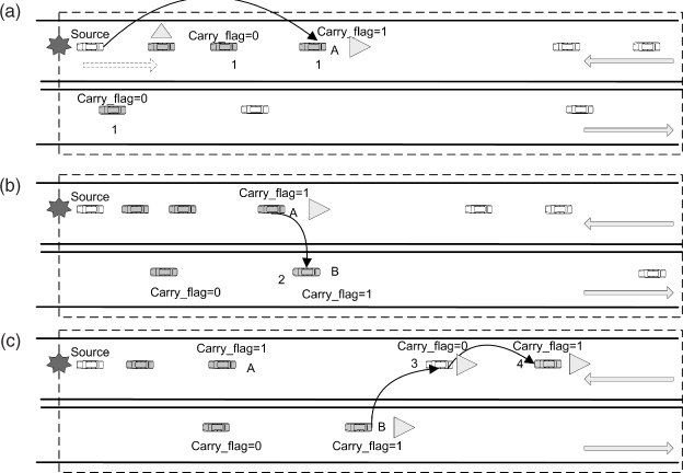
1. We assume the source vehicle is west-bound in the following. For any forwarder (or source) F driving towards west, upon receiving a WM m for the first time, if its locally estimated traffic density (![]() ) is smaller than a threshold density ρth or there are no vehicles in the message direction (east), it will carry the packet and set a carry_flag = 1. (For example, the node A in Figure 10.6(a)). Only if F receives a BACK from a relay in the east will it set carry_flag = 0. If F has not received such a BACK after it retransmits m MAX_RETX times, it will store the packet. Later when F receives a beacon message from a vehicle driving opposite and also located in the east of F, if carry_flag = 1, a rebroadcast of m will be triggered and exactly the same OBCF is invoked (Figure 10.6(b)). Note that, the other node is very close to F because the beacon rate is usually high (for example, ten beacons/s), thus the single-hop reliability is very high in this case.
) is smaller than a threshold density ρth or there are no vehicles in the message direction (east), it will carry the packet and set a carry_flag = 1. (For example, the node A in Figure 10.6(a)). Only if F receives a BACK from a relay in the east will it set carry_flag = 0. If F has not received such a BACK after it retransmits m MAX_RETX times, it will store the packet. Later when F receives a beacon message from a vehicle driving opposite and also located in the east of F, if carry_flag = 1, a rebroadcast of m will be triggered and exactly the same OBCF is invoked (Figure 10.6(b)). Note that, the other node is very close to F because the beacon rate is usually high (for example, ten beacons/s), thus the single-hop reliability is very high in this case.
2. For any vehicle V driving towards east, upon receiving WM m from a forwarder F, if F's local traffic density ![]() (contained in m), V will temporarily set carry_flag = 1. It does not matter whether carry_flag = 1 or 0, if the number of neighbors in the east is larger than 0, V participates in relay selection as usual. This is to let the WM propagate to the end of a “cluster” as fast as it can and to reduce the total transmission count. If carry_flag = 1, only when V later receives a BACK from another relay in the east and also driving towards east will V set carry_flag = 0. Otherwise, if sometime later V receives a beacon message from a node in the east but driving towards the west, FFD will be triggered at V according to OBCF (Figure 10.6(c)). If V is the head of a cluster driving east, V will always carry the WM, and thus reliability is ensured with high probability.
(contained in m), V will temporarily set carry_flag = 1. It does not matter whether carry_flag = 1 or 0, if the number of neighbors in the east is larger than 0, V participates in relay selection as usual. This is to let the WM propagate to the end of a “cluster” as fast as it can and to reduce the total transmission count. If carry_flag = 1, only when V later receives a BACK from another relay in the east and also driving towards east will V set carry_flag = 0. Otherwise, if sometime later V receives a beacon message from a node in the east but driving towards the west, FFD will be triggered at V according to OBCF (Figure 10.6(c)). If V is the head of a cluster driving east, V will always carry the WM, and thus reliability is ensured with high probability.
Figure 10.6 Dissemination process of a WM in the OppCast-extension for the sparse VANET. Legends are the same as for Figure 10.2. © 2011 IEEE. Reprinted, with permission, from Z. Yang, M. Li and W. Lou, “CodePlay: Live Multimedia Streaming in VANETs using Symbol-Level Network Coding”, IEEE Transactions on Mobile Computing (TMC), 2011.
In the above way, the WM can be still disseminated with high speed in connected clusters, where “connected” should be interpreted in probabilistic sense, under opportunistic forwarding and retransmissions. For “disconnected” parts, the opposite directional vehicles act as data mules. Here we need to determine a suitable ρth. If ρth is too small, a WM may not be able to get through the network which affects the PRR; if ρth is too large, there will be redundant rebroadcasts by data mules. We will therefore discover the optimal ρth in Section 10.6.
10.5.5 Implementation Issues
We first give the definition of “neighbors” adopted in the implementation. For a node v to become a neighbor of node u, u needs to receive at least one beacon message from v recently within a reasonable amount of time, such as five times the beacon broadcast interval.
In addition, we need to ensure that the receivers of each (re)broadcast agree on a unified RCR to determine whether to participate in contention processes. We therefore include the locally calculated (optimal) forwarding range of the sender in every broadcast packet from a forwarder/source and each node that receives the packet uses the received value in the packet instead of its own. For the additional makeups to decide their RCRs, they simply rely on the locations of previous visited nodes piggybacked in the rebroadcast packets.
Next, we present the format of the WM packet header in Figure 10.7. The first 2…19 bytes are used for FFD phases, and 20…4k + 29 bytes are used for MFR phases, where k is the maximum level of makeups in a one-hop zone. The fields xleft and xright stand for the boundary locations of the current one-hop zone or sub zone. The list of locations of visited nodes in current one-hop zone include the left and right forwarders, and visited makeups; it is used in MFR to calculate the APRP. Although when k = 2 the header length is 37B, it is relatively small compared to the message length, which is usually more than 200B.
Figure 10.7 The WM packet header format. © 2011 IEEE. Reprinted, with permission, from Z. Yang, M. Li and W. Lou, “CodePlay: Live Multimedia Streaming in VANETs using Symbol-Level Network Coding”, IEEE Transactions on Mobile Computing (TMC), 2011.

In the BACK messages, headers include little information: the one-hop zone index, makeup level, and the sub zone index. The one-hop zone index increases by one when the WM traverses another forwarder, and upon receiving a BACK, a node can determine whether to cancel its own rebroadcast. In practice, in order to enhance the reliability of BACK to suppress redundant transmissions, an additional rule is used. The BACK from a forwarder with a one-hop zone index k + i, i ≥ 0 suppresses the forwarder candidates in the kth one-hop zone, and a higher level makeup suppresses lower level ones in the same one-hop zone.
The pseudo-code of the OppCast protocol at a running at node u is given in Algorithm 10.1.