7.4 Background on Symbol-Level Network Coding

In this section, we first describe the symbol-level network coding technique. Then, we give a motivating example to show the potential advantage of exploiting symbol-level diversity in MCD in VANETs.

7.4.1 A Brief Review of SLNC

Symbol-level Network Coding was recently introduced by Katti et al. (2008) to improve the unicast throughput in wireless mesh networks. It arises from the observation that in wireless networks, even if a packet is received erroneously, some small groups of bits (“symbols”) within that packet are likely to be received correctly. SLNC gathers these correctly received (i.e., “clean”) symbols aggressively, and performs network coding on the granularity of symbols. In contrast to PLNC, SLNC gains from both symbol-level diversity and network coding. In addition, since more bit errors are tolerated than PLNC, SLNC can also gain higher throughput by encouraging more aggressive concurrent transmissions.

In general, SLNC works as follows. A symbol is defined as a group of consecutive bits in a packet, which may correspond to multiple PHY symbols of a modulation scheme. Assume the source has K packets to send, each of them expressed as a vector with elements from a Galois field . The jth symbol in a coded packet at the source is a random linear combination of the jth symbol in all K source packets:

7.1

where is the jth symbol (at jth position) in the ith original packet, coefficient vi is randomly chosen from , and is the coding vector of the coded packet, which is also the coding vector for each symbol. Each receiver node v maintains a decoding matrix for every symbol position. A newly received coded symbol for position j is called innovative to v, if that symbol increases the rank of the decoding matrix of the jth symbol position, referred to as symbol rank. Only innovative clean symbols are buffered.

Each coded packet transmitted by a relay node consists of random linear combinations of buffered clean symbols. For a source, every symbol in a packet is clean and shares the same coding vector. However, at a relay node, coding vectors may be different across symbols. For a coded packet to be sent by relay u, the jth coded symbol is expressed as

7.2

where R is the number of buffered clean symbols at position j, is the ith buffered clean symbol (row) at position j (column), and is the coding vector for that symbol. is the jth symbol of the lth source packet. From Equation (7.2), is still a random linear combination of source symbols and its new coding vectors are .

In the extreme case, every symbol's coding vector is different and needs to be sent along with a packet, which incurs high overheads. To minimize these overheads the optimized run-length coding method can be adopted (Katti et al. 2008), where consecutive clean symbols are combined into a “run”.

We use a three-node toy example to demonstrate how SLNC works (Figure 7.4 and Figure 7.5). The corresponding topology is shown in Figure 7.4. Assume source S has two original packets X and Y to broadcast. Assume a simple scheduling: S broadcasts coded packets until V1 can decode the original packets, and then V1 broadcasts until V2 decodes all original packets.

Figure 7.4 The topology for the example in Figure 7.5. Left: numbers on the edges (links) show the symbol error probabilities; right: corresponding packet error probabilities. Reproduced by permission of © IEEE 2011.

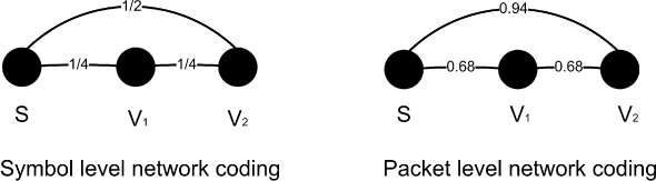
Figure 7.5 Symbol level network coding in VANET content distribution. S: source node; V1 and V2: downloading vehicles and relays. Reproduced by permission of © IEEE 2011.

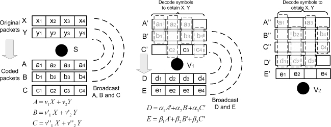
Suppose S generates and broadcasts three coded packets A, B and C, each of them divided into four symbols. Let the symbol error probability from S to V1 be and it happens that each packet received by V1 contains an erroneous symbol (Figure 7.5). Luckily, at least two clean symbols are received for each symbol position. Since any two coding vectors among of A, B and C are independent2, V1 can decode X and Y by solving four linear equations. When V1 broadcasts two packets (say, D and E), it generates two new coded symbols at each position, and packs the eight coded symbols into D and E. Each new coded symbol is also a random linear combination of original symbols. Thus, V2 can recover all original symbols after collecting two innovative coded symbols at each position, which may come from both S and V1.

Next, we show the potential performance gain of SLNC compared with PLNC from two aspects: higher throughput and higher spacial reuse. We use both theoretical analysis and simulation to confirm our intuitions.

7.4.2 Motivation: Why VANET Content Distribution Benefits from SLNC

7.4.2.1 Symbol-Level Diversity that Leads to Higher Throughput

The key insight of SLNC is that, for each symbol position, every correctly received coded symbol is equally useful for decoding, or it does not matter which symbol is received. For PLNC, the reception granularity is a whole packet. The symbol error rate will be much less than the packet error rate, so it is not hard to imagine that SLNC will take less transmissions to collect the information needed for decoding the same amount of content.

To confirm the above intuition, we reuse the above toy example. We would like to compute the expected number of packets () transmitted by S for node V1 to decode using the simple example. Without loss of generality, we assume S has K source packets to broadcast, and each packet is divided into M symbols. We are interested in when V1 is able to decode all the source symbols from S (receive at least M correct and innovative symbols in all the positions). Assume all symbols in the same position are independently received according to an i.i.d. Bernoulli process3, where the probability of receiving a symbol correctly in one trial is 1 − Pse, (Pse = Pse(S, V1)). Let Zi denote the number of packets sent (trials) for V1 to receive exactly K correct symbols in the ith position. Then

7.3

and we have . Define r.v. Z as the smallest number of packets sent for V1 to receive at least K correct symbols at all positions, then

We have

7.4

Therefore, the expected number of packets transmitted by S for Vi to decode is:

7.5

Plugging in the parameters in the example (K = 2, M = 4, Pse = 1/4), we obtain . That is, 3.67 coded packets should be sent by S on average for V1 to decode X and Y.

Next we compare SLNC to using PLNC for the same case. We compute the expected number of packets sent by S for V1 to receive K source packets. Since PLNC discards a packet with any erroneous symbol in it, the error probability from the packet level could be much larger than that of symbol level. For simplicity, we assume independent symbol error in one packet4, so

7.6

The resulting error rates are shown in the right of Figure 7.4 where Ppe(S, V1) = 0.68. Assuming independent packet reception, . For the simple example, S must transmit packets on average for V1 to decode. Thus, the number of transmissions (proportional to downloading delay) of V1 has been reduced by due to the use of SLNC.

For node V2, although it can overhear useful information from both S and V1, as we can see from Figure 7.4, Ppe(S, V2) = 0.94 ≈ 1, while Pse(S, V2) = 1/2. In this case, the (S, V2) link can almost be neglected for PLNC, and SLNC is expected to achieve higher gain for V2 than V1.

From the above, the advantage of using SLNC than PLNC is evident for content distribution in VANET, i.e., it leads to higher downloading rate and incurs fewer transmissions5.

7.4.2.2 Higher Spacial Reusability that Leads to Higher Throughput

In multihop wireless communications, the distances between concurrent transmitting nodes play an important role in achievable network capacity. Another property that has been observed by Katti et al. (2008) is the higher spacial reusability offered by SLNC. However, Katti et al. (2008) only investigated this issue in a static wireless mesh network setting, while we further study this property in the mobile VANETs.

Here the fundamental question is, with SLNC, what is the optimal distance between two nearby relay nodes so that the concurrent transmissions of all relays achieve highest average downloading rate? That is, what is the maximum spacial reusability that can be achieved? Intuitively, if the relays are far away from each other, there is no interference but the space is not fully utilized; but if they are too close, severe interference will in turn decrease the downloading rate. First we define a quantity that reflects the average downloading rate in the network (assume all contents are useful for simplicity):

Definition 7.1 (Average Symbol Reception Probability) (χ(v1, v2, …, vn)) For n relay nodes v1, v2, …, vn in the network, the average probability that every vehicle receives one symbol correctly from any of them during unit time (e.g., the period of one symbol's transmission).

A simple case. To derive χ, let us first consider a toy scenario where there are only two relays v1, v2 in the network. We are interested in the relationship of average symbol reception probability with the inter-relay distance, and when concurrent transmission can gain advantage over nonconcurrent transmission (i.e., two relays transmit separately and alternatively). The following characterizes the condition when concurrent transmission is better than separate transmission:

7.7

where αc is denoted as “concurrency gain.” χ can be derived from symbol error probability (Pse) at each receiving node. However, it is hard to obtain the closed-form solution of Pse under concurrent transmissions (see Li et al. 2010). Therefore, we approximate χ by the average symbol reception ratio:

7.8

which is obtained through Monte Carlo simulations. Given relays v1 and v2, for each of their neighbors w, the received signal to noise ratios (SNRs) are randomly sampled from Nakagami fading model (Li et al. 2010), based on which the signal-to-interference-and-noise ratio (SINR) γ is computed. Successful symbol reception has the probability 1 − Pse|γ, where Pse|γ is the symbol error rate given SINR γ. To simulate packet capture effect in reality6, we let w receive the clean symbols in a packet from v1 if its average SINR , and vice versa. Note that this estimation is done in the worst case, i.e. the relays transmit simultaneously so that every symbol is possibly subject to interference.

For convenience of illustration, we define the following ranges under free space propagation model (Friis): 1. “energy detection range” (ER) (or carrier sensing range) for a transmitter, within which nearby nodes can detect its signal energy. We have , where ThER is the carrier sensing threshold, Tp is the transmission power and G is the antenna gain. 2. The “data communication range” (CR), in which nearby nodes can receive a data packet correctly. , where ThCR is the data reception threshold. Normally ER ≥ CR. These ranges imply statistical transition points across which nodes have different reception results.

We generate ten random topologies for VANET on a highway with traffic density 100/km, fix relay v1 and change v2's position. Each of v1 and v2 transmits ten packets (each having 30 symbols). The number of received symbols is recorded for every node in the network. We also compare with PLNC under the same setting. χ(v1, v2) under the concurrent case is compared with [χ(v1) + χ(v1)]/2 under the nonconcurrent case, against a changing interrelay distance.

The results are given in Figure 7.6. It can be seen that, for SLNC when d(v1, v2) = 2250 m, the concurrency gain αc ≈ 2; when d(v1, v2) decreases, αc monotonically decreases until it becomes smaller than 1, at a small cross-distance dc. While for PLNC, the average packet reception ratio is much smaller, and its cross distance is larger, which shows PLNC's inferior tolerance with concurrent transmission than SLNC.

Figure 7.6 The effect of concurrent transmission of two relays. CR = 250 m, ER = 700 m, data rate: 12 mbps.

The n-relay case. The results of multiple (n > 2) relay nodes transmitting concurrently are based on that of the simple case. Without loss of generality, we assume that vehicles are uniformly distributed and are not too sparse so that neighbor conditions are similar. And n relays are assumed to lie on a straight highway (of length ) with equal interdistance d.

Now we derive the relationship of χ(v1, v2, …, vn) with χ(v1, v2). Let dc = d(v1, v2) when αc = 1 in the simple case. This point can be interpreted equivalently as half of the nodes around each relay are heavily subject to interference while the rest are not. Assuming uniform vehicle distribution, since dc is larger than CR (Figure 7.6, most of these interfered nodes locate in the region between v1 and v2. We are interested in d(v1, v2) > dc, when approximately only the nodes within that region experience a decrease in their symbol reception probabilities. Therefore, a third relay v3 adds little interference to the region between v1 and v2, which is illustrated in Figure 7.7.

Figure 7.7 Conceptual illustration of the n-relay concurrent transmission and calculation of average symbol reception probability.

By assumption, , so

7.9

where , and αc is a function of d and CR. For each CR, αc is obtained by simulation and curve fitting. Since αc is increasing w.r.t. d, χ(v1, v2, …, vn) has a maximal point.

To see the throughput gain of SLNC versus PLNC, Figure 7.8(a) shows the average symbol reception probability χ(v1, v2, …, vn) as a function of D. We can see that with SLNC, for the given example communication range CR = 277m, the optimal distance dopt ≈ 900 m when Pravg is maximized, and Pravg is above 0.5. While with PLNC, dopt ≈ 1200 m, under which Pravg < 0.2. This observation confirms that SLNC tolerates transmission errors better than PLNC. In addition, SLNC allows better spacial reusability and encourages more aggressive concurrent transmissions, thus achieving higher bandwidth efficiency. We find similar conclusions under other communication range CR values, as shown in Figure 7.8(b).

Figure 7.8 Comparison of spacial reusability of SLNC and PLNC. (a) The expected symbol/packet reception rate, for CR = 277 m, ER = 700 m, Data rate = 12 mbps. Nakagami fading model. (b) The optimal distance between two adjacent relays under various data communication ranges. Reproduced by permission of © 2010 IEEE.

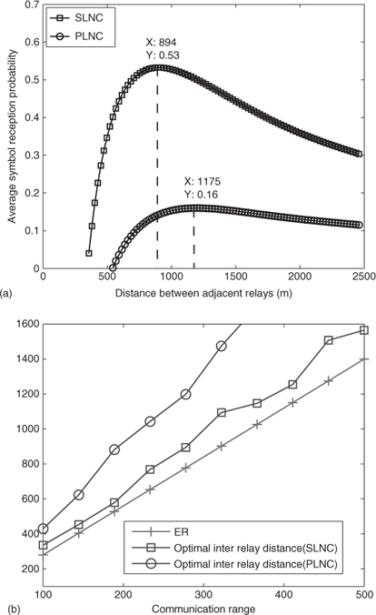
The observations from the above are: 1. the optimal dopt when using SLNC is always smaller than that when using PLNC, and 2. it is interesting to see that dopt for SLNC is very close to energy detection range ER (or carrier sensing range). As we know, the hidden-terminal problem is a major cause of packet collisions for broadcast in a multihop wireless network (Ni et al. 1999; Talucci et al. 1997; Ye et al. 2002). The fundamental reason for the existence of the hidden-terminal problem is the fact that, for wireless packet transmission, the interference range is typically close to or larger than the carrier sensing range. Therefore, it is hard for a localized protocol, especially broadcast/multicast protocols, to eliminate hidden terminals based on local carrier sensing alone. With SLNC, we observed that the concurrent transmission can be successful when nodes are only ER distance apart.

The implication of this observation is significant–with SLNC, we can base the channel access decisions largely on carrier sensing, which is not the case for packet based transmissions that must consider hidden terminals. This property of SLNC was also noticed by Brodsky and Morris (2009) but was not thoroughly investigated. Its great potential to alter the content distribution protocol design, simplify the MAC protocol design and at the same time achieve higher throughput are explored by both of our proposed schemes in this chapter.