CHAPTER 9
Data Science: Making It Smart
Data science is becoming more prominent in everyday analytical exercises, especially around big data. A good example of this is in the car industry. Your local car dealership may be paying for anonymized search data to understand what cars you might want to purchase. In Jacob LaRiviere's article, “Where Predictive Analytics Is Having the Biggest Impact,” he writes about a car dealership leveraging big data and data science to optimize inventory.
By applying data science, we derive greater insight from the information that can be used to guide someone to potentially overlooked opportunities and issues. In the case of the car dealership, they extract web search data for each dealership location to understand what cars are in higher demand in those locations, thereby adjusting stock levels due to anticipated demand.
To empower your analytics, you need to use data science techniques. Data science helps you turn information into insights that are actionable by employing techniques from many fields, including statistics, operations research, information science, and computer science. There are numerous data science techniques, including visualization, predictive modeling, forecasting, data mining, pattern recognition, artificial intelligence, and machine learning. Each of these techniques relies on data, including structured and unstructured data, with a focus in today's world on big data.
For now, let's look at each technique as a tool, or Lego piece, we can use when assembling an analytical solution. We focus on techniques that any practitioner can use to drive business value, often with the help of a data scientist. We will provide an overview of the techniques to give you context for how best to utilize each of these to create your monetization strategy. Several of the techniques have deep disciplines, but a general understanding is all you need to get started.
In this chapter we will cover:
- Metrics
- Thresholds
- Trends and Forecasting
- Correlation Analysis
- Segmentation
- Cluster Analysis
- Velocity
- Predictive and Explanatory Models
- Machine Learning
Metrics
Let's start with a basic technique for any analysis, the metric. A metric is some unit of measurement that enables a manager to process information. The metric can be something as simple as gross sales or as complicated as the beta of a stock. You may hear the terms measure and metric thrown around in the same sentence as most people use them interchangeably. We are not too picky about the use of the two terms, but we do feel compelled to point out the difference.
A measure is a size, amount, or degree expressed in a numeric value. For example, a company's Earnings is a single number for how much the company earned in a particular time period. A metric is defined as a combination of two or more measures. Let's take an example of a common metric of valuation for a company, the price-to-earnings (P/E) ratio. The P/E ratio is calculated by taking two measures, stock price divided by the company's earnings, to assemble a quick reference point to the valuation of the company. Companies are perceived to be inexpensive if they have low P/E ratios, and overpriced if they have high P/E ratios. You can ask someone to perform the math on their own, or provide a metric that provides relative scale for quick evaluation.
When calculating metrics, it is important to define and differentiate between four categories of metrics: key performance indicators (KPIs), success metrics, diagnostic metrics, and operational metrics. The distinction is important to enable the information user's ability to derive relevancy from the analysis. If we overburden the analysis with too many metrics, we may unwittingly cause analysis paralysis and confusion.
A great example of this comes to us from behavioral economics and choice architecture. Behavioral economics leverages a method of economic analysis with psychological insights to explain decision making. Alain Samson, PhD, defines it thus: “Behavioral economics uses psychological experimentation to develop theories about human decision making.” A part of behavioral economics is Choice Architecture, first defined by Richard Thaler and Cass Sunstein in their 2008 book, Nudge: Improving Decisions About Health, Wealth, and Happiness. An example of choice architecture can be found at Google's cafeteria, where management implemented choice architecture to help employees adopt healthy eating habits. They posted a sign informing employees that people who choose larger plates tend to overeat. Due to this simple change, they saw an increase of 50 percent in small plate usage.
While Google still provided two options, a smaller or larger plate, they helped people make the better choice. In our solutions, we can implement choice architecture through the metrics we choose in our solutions. It will directly impact the usability of the analytical solution and type of choices and decisions it empowers.
There is also the “so-what?” factor if you provide too many metrics. The metric may be interesting, but if it is not used or does not drive an action, we question whether to deploy it in our solution.
Let's take a look at our four categories of metrics:
- KPI—A key performance indicator can be thought of as an organizational metric that is used to determine progress on goals at all levels in the organization. These should be limited to five to seven top KPIs that align to the business's objectives and goals. An example might include Revenue, Units Sold, or Net Profit.
- Success Metrics—We leverage success metrics to drive our decisions in our monetization strategy. As we discussed in the Decision Analysis chapter (Chapter 4), our success metrics are those that a managers can utilize to inform themselves about what decision to make. We usually uncover the success metrics at the end of a process of determining the questions, decisions, actions, and metrics that a manager makes on a particular topic.
- Diagnostic Metrics—Diagnostic metrics are specific metrics for a particular subject area, department, or capability. These metrics help us further diagnose an issue or opportunity. In addition to success metrics, they should be linked to a particular decision and drive action, but not always.
- Operational Metrics—These are the most basic metrics used to monitor or analyze the performance of a business process. They form the foundation for diagnostic and success metrics but are typically too narrow to rise to the top in an analytical solution.
Let's use the Edison Credit Card Company, which issues credit cards through the Internet, direct mail, and affiliate marketing, as a fictional example. We are charged with building an analytical solution for the company and need to bucket the following 10 metrics into our paradigm of four metric types.
- Acquisition Cost per Customer
- Email Marketing Click-Through Rate
- Database Server Utilization
- Customer Attrition Rate
- Average Revenue per Customer
- Affiliate Marketing/Finance Website Channel/Number of Referrals
- Average Direct Mail Response Rate
- Direct Mail/College Campaign/Response Rate
- Average Interest Rate
- Charge Off Percentage to Revenue
There are some clear winners for each of the buckets and there are several metrics that may be fungible depending on the analytical need. Clearly metric number 3, Database Server Utilization, is in the operational category. For the KPI bucket, numbers 1, 4, 5, and 9 all qualify as high-level metrics that drive the organization's performance. Metric numbers 6 and 8 are best suited for a specific diagnostic and therefore go into the diagnostic metrics bucket. For success metrics, metrics numbered 2, 6, and 10 are strong candidates.
Again, the purpose is to determine what metrics truly drive insights and actions relevant to the stated hypothesis and business objectives. A lot of analysts and data scientists can get lost in creating metrics that are not used or actionable. Horticulturists are fond of saying that a weed is simply a misplaced plant. We can view metrics in a similar manner. Placing the right metric with the right analytical solution is the goal.
Thresholds
Once our metrics are defined, we add additional relevance to assist the manager with the ability to quickly decide if there is an opportunity or issue. We think of this as a threshold or a boundary range that is triggered when the metric falls outside of this range. It is the signal to the information user that further diagnostics may be needed or it is time to take action.
An example of how a threshold can be a signal for further investigation can be found at Intercontinental Hotel Group (IHG), where they have built a set of diagnostic analytical solutions that allow a user to determine if individual hotels are leveraging forecasting strategies to optimize occupancy. Once a certain threshold is hit, a visual alert is triggered, signaling the need for reforecasting.
To implement a threshold, let's return to our fictional example of the Edison Credit Card Company. If we know that our average Customer Attrition Rate is 15 percent a year, we may determine that a 2 percent variance is okay. We know that if this metric rises to 18 percent in any given time period, we need to investigate immediately to understand why attrition seems to be rising and what is occurring with the business or marketplace in order to take action. Here are some questions the manager may ask to diagnose the issue:
- Has the market moved to a lower interest rate and our credit card product is no longer competitive?
- Did we charge off a large number of bad customers, causing a spike in attrition?
- Is there a particular credit card product that is causing the bulk of the attrition spike?
To determine an acceptable variance range, you may deploy a few techniques from various sources. The company's financial analyst may determine these are the limits in order for the company to reach its financial targets. The variance may be an industry norm against a competitive set that typically sees a range of customer attrition between 13 and 17 percent. Another option is an analysis from a data scientist determining that the standard deviation from historical attrition rates for the company varies by 2 percent within a given year.
Let's take a look at standard deviation for this example as it might be more the norm if no clear threshold amount is apparent in the data. Standard deviation is a metric to quantify variation in a dataset. If the standard deviation is low, it suggests that the dataset points are close to the mean. A high standard deviation indicates that the variation in the dataset is dispersed over a wider range.
One standard deviation in the dataset will encompass roughly 68 percent of the distribution, which might be an initial tolerance level when you begin to determine the needed threshold for a metric. If a metric value falls out of the 68 percent expected range, we know that there might be an issue or opportunity. In this case, the standard deviation has been calculated as 1.129 percent based on a 15 percent average attrition rate. If the attrition rate rises above 16.129 percent, an alert will trigger, notifying the analyst that there may be an issue requiring further investigation. Given that attrition is undesirable, you are primarily concerned when the rate exceeds the upper bound of our threshold.
Trends and Forecasting
Trends are a series of data points for a particular metric to show performance over time. In the diagnostic process, an analyst wants to quickly surmise if the issue is a onetime anomaly or a systemic concern that warrants further diagnosis. Forecasting is the ability to use historical data to determine the most likely outcome or outcomes in the future. Both trend analysis and forecasting can be used by the manager to dig deeper into a metric to determine if a pattern exists that can be leveraged to take advantage of an opportunity.
Weather forecasts powered by Monte Carlo simulations are an excellent example of forecasts. In today's world, storm trackers don't rely on a single forecast; they utilize many potential scenarios to understand the probability that a storm will take a particular path. Monte Carlo simulations select many data points for a given situation and produce a range of potential outcomes. For Hurricane Sandy over 50 different scenarios were run with over 10 million randomized atmospheric variables to determine the possible landing point, enabling a 20-hour window to alert residents to evacuate.
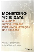
To further build on our fictional example, let's take the Edison Credit Card Company and look at how trend and forecasting may be employed. Customer Attrition Rate is a key metric measuring the churn of customers on a monthly basis. Taking one month as a data point for a decision may mislead the analysis. If a manager receives a reading that the current month of July has an attrition rate of 18.8 percent and the average is 15 percent, they have good reason to be nervous.
However, the manager will probably want to know if the issue is systemic or just an anomaly. At this point, a trend is a good tool that can provide more context to the metrics. In Figure 9.1, we see a five-month prior history along with a forecast for the next few months, August through October. With this new perspective, the manager is more likely to be at ease with the onetime anomaly.

Figure 9.1 Customer Attrition Rate (Annualized)
Correlation Analysis
Another key technique to assist you with determining the relevance of a metric is correlation analysis. A correlation is an association between two or more metrics where a linear dependency or relationship exists, but correlation does not necessarily mean causality. An actionable relationship is the key determinant for our purposes.
What does this mean? Correlation is determining what things happened together. Causality is trying to determine why something happened. A great example comes from an article by David Ritter, “When to Act on a Correlation, and When Not To.” He contemplates the importance of correlation and causality when determining whether to take action based on risk and confidence in the relationship. In this example, the NYC Health department monitors the city for violations and has deployed sewer sensors to collect readings.
This is a good example where casualty may be hard to determine, but with correlations and confidence in the meaning of the data, action for further investigation was taken. By sending out an investigative unit they may be able to determine the cause.
To find correlations that exist in the data, it is helpful to interview subject matter experts (SMEs) to gain an understanding of learned business rules and correlations that are institutional knowledge. These learnings are often the starting point for deeper analysis. We should take care to validate the insight gained from an SME, as organizational wisdom can be dated, inaccurate, or influenced by a cognitive bias. However, these are great starting points to investigate further through data science.
Another approach is to begin with a data scientist digging into a dataset to look for relationships. One approach is the Pearson's Correlation Coefficient (or simply correlation coefficient). It is obtained by dividing the covariance of the two variables by the product of their standard deviations. Let's briefly review the covariance and correlation coefficient:
- Covariance, a measure of how two variables are linearly related, is calculated by taking the average of the product of deviations (differences) of the two variables from their own averages:

- Correlation coefficient (
 is a scaled, unitless version of covariance. It is obtained by dividing the covariance of two variables by the product of their respective standard deviations, and can range from –1 to 1:
- A correlation of –1 indicates the two variables are perfectly negatively associated (a unit increase in one variable is associated with a unit decrease in the other).
- A correlation of 1 indicates the two variables are perfectly positively associated (a unit increase in one variable is associated with a unit increase in the other).
- A correlation of 0 indicates there exists no linear association between the two variables.
- In Figure 9.2, (a) illustrates strong positive correlation, (b) strong negative, and (c) no linear correlation. In (d), the correlation coefficient is also 0, indicating no linear correlation—but clearly a curvilinear relationship exists (y = –x2).

Figure 9.2 Correlation Examples
Segmentation
Dividing organizations' customers, markets, and/or channels into groupings of similar characteristics or behavior is known as segmentation. The purpose of segmenting a population of data can be for a variety of reasons. One reason may be to further refine and target marketing activities to drive up relevance of a message. Another might be to segment customers in categories to determine profitability and potential. The basic premise of segmentation is by grouping your customer into the right segments you can target a specific message that would drive a lift in sales due to higher relevance of your message.
An analytic dataset typically has many characteristics useful for segmentation. For example, the attributes in a demographic segmentation may include: geography, age, income, education, and ethnicity. If an organization does not already have customer, market, or channel segments, this method can be of great use to find areas to monetize underserved segments. If an organization already leverages segmentation, there may be additional opportunities to further carve out sub-segments to drive additional revenue lift, assuming these sub-segments are commercially feasible.
Segmentation can also include letting customers self-select into a segment based on purchasing behavior. In Gretchen Gavett's article, “What You Need to Know About Segmentation,” she writes about how her company, Quidol, markets their early pregnancy test:
There was a $3 price difference in the two products, even though they were the same core product. The cheaper version, or “fearfuls,” was marketed in a mauve background with no baby on the box, located near the condoms. The “hopefuls,” the more expensive version, was marketed in a pink box with a smiling baby, located near the ovulation-testing kits. Based on the life experience of the individual purchasing the pregnancy test, they can opt into the segment that best fits them.
Let's take a look at our fictional example, the Edison Credit Card Company, to further refine this concept. From Edison's metrics that we reviewed earlier in the chapter, we infer they already have Customer and Channel segments. From the Affiliate Marketing Number of Referrals for the Finance Website metric we deduce they have channel segments and that one of the channels is Financial Websites. From the Direct Mail/College Campaign/Response Rate metric, we determine they have customer segments and have one targeted to college students.
After a few questions, we determine that they do not segment their customers based on a particular geography. After analyzing the company's campaign management and sales data, we identify five geographical segments with the following click-through and conversion data points (see Table 9.1).
Table 9.1 Marketing Effectiveness Decision Matrix
| Segment | Emails Sent | Click-Through | Click-Through Rate | Conversions to Purchase | Conversion Rate |
| Northeast | 352,488 | 16,214 | 4.60% | 519 | 3.20% |
| Southeast | 232,101 | 14,390 | 6.20% | 463 | 3.50% |
| Midwest | 177,033 | 6,727 | 3.80% | 161 | 2.40% |
| West | 483,282 | 24,744 | 5.12% | 297 | 1.20% |
| Canada | 58,972 | 2,831 | 4.80% | 113 | 4.00% |
From this analysis, we decide to focus more of our efforts on the Northeast and Southeast regions. We look for affiliates in these areas to partner with to drive more referrals. In addition, we place higher priority on our marketing activities and spend in these regions. This exercise shows that by segmenting the data, we find opportunities for additional revenue the company can drive.
Many segmentation exercises have more than one dimension. For example, in Figure 9.3 we create four segments that have Income, Household Size, and Age as segment dimensions to create their segmentation strategy. Multidimensional segmentation models are more complex to develop and comprehend, but the principles behind them are the same. Their purpose is to answer the questions, “How do we group our customers to best target sales and marketing activities to them?”

Figure 9.3 Multidimensional Segmentation Model
Cluster Analysis
Cluster analysis is the grouping of like data points that are “similar” across enough characteristics to form a cluster and significantly “different” from other data points with respect to the same characteristics. Clustering is similar to segmentation, but is machine-learned and more mathematically intensive than segmentation.
For example, you may have a clustered approach around the propensity to purchase or likelihood to purchase a companion product. Marketers often use demographic characteristics of shoppers or locations to form clusters to better understand the different desires, needs, and behaviors of consumers in a marketable way (see Figure 9.4).

Figure 9.4 Cluster Analysis Example
These data-driven clusters can be profiled with behavioral or transactional data and used to form market segments against which to action. In this case, we use segments and clusters almost interchangeably, with segments being clusters that are “brought to life” and utilized for marketing.
An example of this can be found at Thomson Reuters Corporation when it made a dramatic transformation into a global information services firm from a paper-based publishing company. In order to turn the corner, the company created segments aligned to the users of their financial products; these included institutional equity advisers, fixed-income advisers, and investment bankers. Next, they leveraged clustering techniques to drive strategic direction within these segments. In Richard J. Harrington and Anthony K. Tjan's article, “Transforming Strategy One Customer at a Time,” they write about the clustering approach:
This approach to clustering helped Thomson Reuters Corporation survive and thrive in the digital transformation that has occurred in the publishing and information industry.
An example of using visual display of information to understand underserved segments can be found at Sean Gourley's company, Quid, where they use semantic-clustering analysis to spot white spaces in competition for possible opportunities. They recently identified an opportunity to link gaming and biopharma together, producing a new market for advertising. “Such maps expose surprising relationships between and across sectors and, even more tantalizing, the white spaces among them—which can offer firms strategic opportunities to connect companies operating in different markets, to take existing products into new sectors, or to innovate with products and services no one has even dreamed up yet.”
Cluster analysis comprises several data-mining techniques. A cluster cannot be universally defined because it is based on natural groupings of characteristics in the data that form a cluster depending on the technique being used. Two of the most common clustering techniques we discuss here are hierarchical and k-means clustering algorithms.
Before we can assign clusters, we determine which of the data points (units/stores, shoppers, consumers, hotels, etc.) are most similar. There are many mathematical ways to do this. For a simple example, we illustrate using stores and their associated shopper demographics (see Figure 9.5).

Figure 9.5 Hierarchical Clustering
Stores 1 and 3 are most similar, or closest, to each other based on shopper area demographics. We use a mathematical “distance” formula to determine similarity and can see this easily in the example data.
But what happens when we have many more stores, and many more characteristics? A statistical clustering algorithm can take into account many more data attributes (i.e., shopper demographics), for thousands of stores, and iteratively determines which stores are most alike within groups (clusters) and most different from other groups (Figure 9.6).

Figure 9.6 K-Means Clustering
Once a method is chosen for calculating the distance or similarity between two units, there are many options for building the clusters.
- K-Means clustering is a nonhierarchical, iterative clustering method that uses “seeds” to initiate the clusters, then iteratively assigns additional units to the same cluster based on similarity to the mathematical centroid of the cluster. The number of clusters (k) must be specified, and the user can use business rules or data-driven optimization methods to select the number. Cluster iterations are independent of each other and data points can be assigned and reassigned in each iteration.
- Hierarchical clustering is different from k-means in that there is no seed to initiate clusters, and each iteration is highly dependent on the others. Once a unit is assigned to a cluster, it cannot switch to another—although clusters may be combined or split, depending on the method. There are two main types:
- Agglomerative—A bottom-up clustering, where each data point starts in its own cluster and clusters are merged until there is a single cluster containing all data points. The user selects the number of clusters that yields the best results, often observing a dendrogram (tree diagram) of the clustering hierarchy.
- Divisive—A top-down clustering, exactly the opposite of agglomerative. We start with a single cluster of all data points, and split based on similarity measures until each data point is in its own cluster, again observing diagnostic statistics or a dendrogram to choose the best number of clusters.
There are several great resources available that go more in depth into these techniques, including:
- Statistical Consulting, 2002 edition, by Javier Cabrera and Andrew McDougall
- Data Science for Business: What You Need to Know about Data Mining and Data-Analytic Thinking by Foster Provost and Tom Fawcett
- Business Statistics: Communicating with Numbers, 2nd edition, by Sanjiv Jaggia and Alison Kelly
Velocity
Another important data science technique is velocity, which determines the rate of change and direction for a particular metric. It helps to understand if a metric is on an uptrend or downtrend. Velocity is similar to trends and forecasting where the business manager is solving for whether an issue is systemic or a onetime anomaly. Velocity is different in that it helps determine the rate of change and direction (up or down) for a metric.
Let's use the Edison Credit Card Company example from our segmentation discussion. We add a Conversion Rate Velocity metric to help us understand the direction for a particular segment. To explain how this works, if our conversion rate is 3 percent and our velocity is 1.0, we expect our conversion rate to maintain at 3 percent. However, if the velocity is 1.1, we expect the 3 percent conversion rate to go upward, possibly to 3.1 or 3.2 percent. If the velocity is 0.9, then we expect the conversion rate to start ticking downward, possibly to 2.8 or 2.9 percent.
Let's take a look at the updated Decision Matrix with Conversion Rate Velocity added.
In Table 9.2, we see that the both Southeast and the West regions are on the downtrend. Canada is expected to remain flat and the Northeast and Midwest are both on the uptrend. Does the Velocity metric change our investment decision?
Table 9.2 Decision Matrix with Conversion Rate Velocity Metric
| Segment | Emails Sent | Click-Through | Click-Through Rate | Conversions to Purchase | Conversion Rate | Conversion Rate Velocity |
| Northeast | 352,488 | 16,214 | 4.60% | 519 | 3.20% | 1.10 |
| Southeast | 232,101 | 14,390 | 6.20% | 463 | 3.50% | 0.95 |
| Midwest | 177,033 | 6,727 | 3.80% | 161 | 2.40% | 1.15 |
| West | 483,282 | 24,744 | 5.12% | 297 | 1.20% | 0.87 |
| Canada | 58,972 | 2,831 | 4.80% | 113 | 4.00% | 1.00 |
In some cases, velocity may be very important; in others, velocity may be interesting, but historical values may change so often that it does not have much meaning for the analytical solution. It is in large part your job as the decision architect to work with the data scientist to determine what Lego pieces fit within the analytical solution you are creating.
Predictive and Explanatory Models
We use statistical models to try to predict or explain a certain behavior by assigning a probability to an outcome. For example, in an acquisition, cross-sell, or upsell model, propensity to purchase may be a score associated with each potential customer based on certain input parameters. The manager may use this score to group the highest likely candidates and apply marketing dollars to that set. Conversely, in a churn or attrition model, the same methods may be used to predict the loss of a customer or subscriber and target the most at-risk groups based on propensity score deciles.
The above examples model a binary outcome (a sale happens or it doesn't). When the outcome is not binary (e.g., realized revenue, rooms booked, inventory sold, mobile data usage, counts of an event, multinomial outcomes, etc.), we use general or generalized modeling techniques such as linear regression, Poisson modeling, and a multitude of others.
Whether the purpose of a model is predictive or explanatory depends on the business question. The approaches between the two types are generally similar, but the application is not. A predictive model is often used for forecasting outcomes in the future, or guessing whether a certain behavior will happen. Sometimes, this is less important than understanding, or explaining, which characteristics of the business, customer, or environment are driving these outcomes—in which case the model becomes more explanatory.
Model accuracy requirements are more relaxed in the case of an explanatory model, as we try to understand directionally what is happening in order to drive change within the business. Predictive models, typically, must be highly accurate to be useful.
A good example of leveraging predictive models along with big data comes from the International Maritime Bureau (IMB), which uses these techniques to catch pirates. For the 2012 year, they were able to drop the reported incidents of pirate attacks for the first half of the year by 54 percent, some of which they attribute to two main factors related to their analytical solution. First, they brought in big data in a flexible analytical environment so that the data can be near real time. This data included interviews with pirates in custody, news stories about piracy incidents, data from mobile phones, email traffic, and social media posts from the pirates themselves. Once advanced analytics was applied to this dataset, Visualization was the next factor. Using geospatial mapping, they were able to visualize pictures to identify, track, and intercept the pirates and their organized networks.
Machine Learning
Machine learning is the next frontier in Data Science and is getting a lot of attention as companies look to incorporate self-learning models to tackle tough business problems. Machine learning is a type of artificial intelligence that provides computers with the capabilities to learn on their own without being explicitly programmed. One important difference in machine learning is that it is focused on prediction, not causality.
Machine learning has high applicability to areas where you are trying to predict an outcome. One example of this is from Eric Horvitz and the team at Microsoft Research, who developed a machine learning model that can predict, with a high level of accuracy, whether a patient with congestive heart failure who is released from the hospital will be readmitted within 30 days. Through machine learning and hundreds of thousands of data points involving 300,000 patients, the machine is able to learn the profiles of those patients most likely to be readmitted. This is leading to patient-specific discharge programs aimed at keeping the patients in stable, safe regimes.
Other examples of how companies are deploying machine learning include personalized recommendations for customers, anticipating attrition of employees, credit scoring of loan applicants, and asset utilization for fleet maintenance. In their article, “How Companies Are Using Machine Learning to Get Faster and More Efficient,” authors James Wilson, Sharad Sachdev, and Allan Alter provide several examples of how companies are increasing performance of certain tasks by 10 times the normal rate. One example cited,
Through the various techniques discussed in this chapter, you should now have a basic understanding of Data Science and its ability to improve your analytical solution. These techniques play an important role in using your data to develop your decision architecture and monetization strategies.