Reducing RAM consumption with check-pointing

We pointed out in Chapter 11 that, due to RAM consumption, AAD cannot efficiently differentiate calculations taking more than 0.01 seconds on a core. Longer calculations, which include almost all cases of practical relevance, must be divided into pieces shorter than 0.01 seconds.core, and differentiated separately over each piece, wiping RAM in between and aggregating sensitivities in the end.

How exactly this is achieved depends on the instrumented algorithm. This is particularly simple in the case of path-wise simulations, where sensitivities are computed path by path and averaged in the end. But this solution is specific to simulations. This chapter discusses a more general solution called check-pointing. Check-pointing applies to many problems of practical relevance, in finance and elsewhere. Huge successfully applied it to the differentiation of multidimensional FDM in [90]. Huge and Savine applied it to efficiently differentiate the LSM algorithm and produce a complete xVA risk in [31]. We explain check-pointing in general mathematical and programmatic terms and apply it to the differentiation of calibration.

Formally, we differentiate a two-step algorithm, that is, a scalar function that can be written as:

where is a vector-valued function and is a scalar function, assumed differentiable in constant time. We denote and .

In the context of a calibrated financial simulation model, is the value of some transaction in some model with parameters . We learned to differentiate in constant time in the previous chapter. is an explicit¹ calibration that produces the model parameters out of market variables , with . computes the value of the transaction from the market variables . The differentials of are the hedge coefficients, also called market risks, that risk reports are designed to produce.

Importantly, there are many good reasons to split differentiation this way, besides minimizing the size of the tape. In the context of financial simulations, intermediate differentials provide useful information for research and risk management, the sensitivity of transactions to model parameters and the sensitivity of model parameters to market variables aggregated into market risks, but also constitute interesting information in their own right. Besides, to differentiate calibration is fine when it is explicit, but to differentiate a numerical calibration may result in unstable, inaccurate sensitivities. We present in Section 13.3 a specific algorithm for the differentiation of numerical calibrations. But we can only do that if we split differentiation between calibration and valuation.

Another example is how we differentiated the simulation algorithm in the previous chapter. We split the simulation algorithm into an initialization phase , which pre-calculates deterministic results from the model parameters , and a simulation phase , which generates and evaluates paths and produces a value out of and .² We implemented in a loop over paths, and differentiated each of its iterations separately, before propagating the resulting differentials over . This is a direct application of check-pointing, although we didn't call it by its name at the time. If we hadn't split the differentiation of into the differentiation of and the differentiation of , we could not have implemented path-wise differentiation that efficiently. More importantly, we could not have conducted the differentiation of in parallel. In order to differentiate in parallel a parallel calculation, we must first extract the parallel piece and differentiate it separately from the rest, applying check-pointing to connect the resulting differentials.

As a final example, we could split the processing of every path into the generation of the -dimensional scenario and the evaluation of the payoff. We differentiated altogether in the previous chapter, but for a product with a vast number of cash-flows valued over a high-dimensional path, like an xVA, we would separate the differentiation of the two to limit RAM consumption.

In all these cases, can be differentiated in constant time with AAD because it is a scalar function. In theory, is also differentiable in constant time because it is also a scalar function. But we discussed some of the many reasons why it may be desirable to split its differentiation. Hence, the exercise is to split the differentiation of into a differentiation of and a differentiation of while preserving the constant time property. The problem is that is not a scalar function, hence it cannot be differentiated in constant time with straightforward AAD. To achieve this, we need additional logic, and it is this additional logic that is called check-pointing.

Formally, from the chain rule:

and our assumption is that we have a constant time computation for . But AAD cannot compute the Jacobian in constant time. We have seen in Chapter 11 that Jacobians take linear time in the number of results . With bumping, it takes linear time in . In any case, it cannot be computed in constant time. Furthermore, is the product of the vector by the matrix , linear in .

Check-pointing applies adjoint calculus to compute in constant time, in a sequence of steps where the adjoints of and are propagated separately, without ever computing a Jacobian or performing a matrix product.

If, hypothetically, we did differentiate altogether with a single application of AAD, what would the tape look like?

It must be this way, because is computed before , and only depends on the results of .

The part of the tape that belongs to is self-contained for adjoint propagation, because only depends on , and not on the details of its internal calculations within .³ So the arguments to all calculations within must be located on 's part of the tape, including ; they cannot belong to 's part of the tape.

The section of the tape that belongs to (inclusive of inputs and outputs ) is also self-contained. Evidently, the calculations within cannot depend on the calculations in , which is evaluated later. And we have seen that the calculations within cannot directly reference those of , except through its outputs .

Hence, the tape for is separable for the purpose of adjoint propagation: it can be split into two self-contained tapes, with a common section as the output to 's tape and the input to 's tape.

It should be clear that an overall back-propagation through the entire tape of is equivalent, and produces the same results, as two successive back-propagations, first through the tape of , and then through the tape of . Note that the order is reversed from evaluation, where is evaluated first and is evaluated last.

It is this separation that allows the multiple benefits of separate differentiations, including a smaller RAM consumption. Only one of the two tapes of and is active at a time in memory, and the differentials of are accumulated through adjoint propagation alone, hence, in constant time. The check-pointing algorithm is articulated below:

1. Starting with a clean tape, compute and store without AAD instrumentation. The only purpose here is to compute . Put on tape.
2. Compute the final result with an instrumented evaluation of . This builds the tape for .
3. Back-propagate from to , producing the adjoints of : . Store this result.
4. Wipe 's tape. It is no longer needed.
5. Put on tape.
6. Recompute as in step 1, this time with AAD instrumentation. This builds the tape for .
7. Seed that tape with the adjoints of , that is the , known from step 3. This is the defining step in the check-pointing algorithm. Instead of seeding the tape with 1 for the end result (and 0 everywhere else), seed it with the known adjoints for all the components of the vector .
8. Conduct back-propagation through the tape of , from the known adjoints of to those, unknown, of .
9. The adjoints of are the final, desired result: .
10. Wipe the tape.

The following figure shows the state of the tape after each step:

It should be clear that this algorithm guarantees all of the following:

• Constant time computation since only adjoint propagations are involved. Note that the Jacobian of is never computed. We don't know it at the term of the computation, and we don't need it to produce the end result. Also note that successive functions are propagated in the reverse order to their evaluation. Check-pointing is a sort of “macro-level” AAD where the nodes are not mathematical operations but steps in an algorithm.
• Correct adjoint accumulation since it should be clear that these computations produce the exact same results as a full adjoint propagation throughout the entire tape for . It is actually the same propagations that are executed, but through pieces of tape at a time.
• Reduced RAM consumption since only the one tape for or lives in memory at a time.

In code, check-pointing goes as follows:

We could write a generic higher-order function to encapsulate check-pointing logic. But we refrain from doing so. It is best left to client code to implement check-pointing at best in different situations. The AAD library provides all the basic constructs to implement check-pointing easily and in a flexible manner.

Note that the algorithm also works in the more general context where:

because, then:

The left-hand side is computed in constant time by differentiation of (we can do that: it has been our working hypothesis all along). The right-hand side is computed by check-pointing.

Alternatively, we may redefine to return the coordinates of in addition to its result , and we are back to the initial case where .

This concludes our general discussion of check-pointing. Check-pointing applies in vast number of contexts, to the point that every nontrivial AAD instrumentation involves some form of check-pointing, including the instrumentation of our simulation library in the previous chapter, as pointed out earlier. In the next section, we apply check-pointing to calibration and the production of market risks. In the meantime, we quickly discuss application to black box code.

Check-pointing black box code

AAD instrumentation cannot be partial. The entire calculation code must be instrumented, and all the active code must be templated. A partial instrumentation would break the chain rule and prevent adjoints to correctly propagate through non-instrumented active calculations, resulting in wrong differentials. It follows that all the source code implementing a calculation must be available, and modifiable, so it may be instantiated with the Number type.

In a real-world production environment, this is not always the case. It often happens that part of the calculation code is a black box. We can call this code to conduct some intermediate calculations, but we cannot easily see or modify the source code. The routine may be part of third-party software with signatures in headers and binary libraries, but no source code. Or, the source code may be written in a different language. Or, the source is available but cannot be modified, for technical, policy, or legal reasons.

Or maybe we could instrument the code but we don't want to. An intensive calculation code with a low number of active inputs may be best differentiated either analytically or with finite differences. Or, as we will see in the case of a numerical calibration, some code must be differentiated in a specific manner, a blind differentiation, either with finite differences or AAD, resulting in wrong or unstable derivatives. This applies to many iterative algorithms, like eigenvalue decomposition, Cholesky decomposition, or SVD regression, as noted by Huge in [93].

In all these cases, we have an intermediate calculation that remains non-instrumented, and differentiated in its own specific way, which may or may not be finite differences.⁴ Check-pointing allows to consistently connect this piece in the context of a larger differentiation, the rest of the calculation being differentiated in constant time with AAD.

For example, consider the differentiation of a calculation that is evaluated in three steps, , , and :

where is the black box. It is not instrumented, and its Jacobian is computed by specific means, perhaps finite differences. The problem is to conduct the rest of the differentiation in constant time with AAD, and connect the Jacobian of the black box without breaking the derivatives chain. We have discussed a walkaround in Chapter 8 in the context of manual adjoint code. In the context of automatic adjoint differentiation, we have two choices.

We could overload and make it a building block in the AAD library, like we did for the Gaussian functions in Chapter 10. This solution invades and grows the AAD library. It is recommended when is a low-level, general-purpose algorithm, called from many places in the software.

In most situations, however, would be a necessary intermediate calculation in a specific context, which doesn't justify an invasion of the AAD library. All we need is a walkaround in the instrumentation of , along the lines of Chapter 8, but with automatic adjoint propagation. We can implement such walkaround with check-pointing. Denote:

then, by the chain rule:

We start with a non-instrumented calculation of , as is customary with check-pointing. Next, we compute the value of , as well as its Jacobian , computed, as discussed, by specific means.

Knowing , we compute the gradient , a row vector in dimension , of , in constant time, with AAD instrumentation. We multiply it on the right by to find:

This row vector in dimension is by definition the adjoint of in the calculation of . We can therefore apply the check-pointing algorithm. Execute an instrumented instance of:

which builds the tape of , seed the adjoints of the results with the known , and back-propagate to find the desired adjoints of , that is .

We successfully applied check-pointing to connect the specific differentiation of with the rest of the differentiated calculation. The differentiation of takes the times it takes, and a matrix-by-vector product is necessary for the connection, but the rest of the differentiation proceeds with AAD in constant time.

Dupire's formula

We now turn toward financial applications of the check-pointing algorithm, more precisely, the important matter of the production of market risks.

So far in this book, we implemented Dupire's model with a given local volatility surface , represented in practice by a bilinearly interpolated matrix. Its differentiation produced the derivatives of some transaction's value in the model with respect to this local volatility matrix.

But this is not the application Dupire meant for his model. Traders are not interested in risks to a theoretical, abstract local volatility. Dupire's model is meant to be calibrated to the market prices of European calls and puts, or, equivalently, market-implied Black and Scholes volatilities, such that its values are consistent with the market prices of European options, and its risk sensitivities are derivatives to implied volatilities, which represent the market prices of concrete instruments that traders may buy and sell to hedge the sensitivities of their transactions.

Dupire's model is unique in that its calibration is explicit. The calibrated local volatility is expressed directly as a function of the market prices of European calls by Dupire's famous formula [12]:

where is today's price of the European call of strike and maturity , and subscripts denote partial derivatives.

Dupire's formula may be elegantly demonstrated in a couple of lines with Laurent Schwartz's generalized derivatives and Tanaka's formula (essentially an extension of Ito's lemma in the sense of distributions), following the footsteps of Savine, 2001 [44].

By application of Tanaka's formula to the function under Dupire's dynamics , we find:

where is the Dirac mass. Taking (risk-neutral) expectations on both sides:

where is the (risk-neutral) density of in , and since , we have Dupire's result:

Similar formulas are found with this methodology in extensions of Dupire's model with rates, dividends, stochastic volatility, and jumps; see [44].

The Implied Volatility Surface (IVS)

Dupire's formula refers to today's prices of European calls of all strikes and maturities , or, equivalently, the continuous surface of Black and Scholes's market-implied volatilities . In Chapter 4, we pointed out that this is also equivalent to marginal risk-neutral densities for all maturities, and called this continuous surface of market prices an Implied Volatility Surface or IVS.

The IVS must satisfy some fundamental properties to feed Dupire's formula: it must be continuous, differentiable in , and twice differentiable in . must be strictly positive, meaning call prices must be convex in strike. We also require that , meaning call prices are increasing in maturity. or would allow a static arbitrage (see for instance [46]) so any non-arbitrageable IVS guarantees that . But this is not enough. We need strict positiveness as well as continuity and differentiability.

We pointed out in Chapter 4 that the market typically provides prices for a discrete number of European options, and that to interpolate a complete, continuous, differentiable IVS out of these prices was not a trivial exercise. The implementation of the accepted solutions in the industry, including Gatheral's SVI ([40]) and Andreasen and Huge's LVI ([41]), are out of our scope here.

We circumvent this difficulty by defining an IVS from Merton's jump-diffusion model of 1976 [98]. Merton's model is an extension of Black and Scholes where the underlying asset price is not only subject to a diffusion, but also random discontinuities, or jumps, occurring at random times and driven by a Poisson process:

where is a Poisson process with intensity and the s are a collection IID random variables such that . The Poisson process and the jumps are independent from each other and independent from the Brownian motion. Jumps are roughly Gaussian with mean and variance . guarantees that satisfies the martingale property so the model remains non-arbitrageable.

Merton demonstrated that the price of a European call in this model can be expressed explicitly as a weighted average of Black and Scholes prices:

where is Black and Scholes's formula. The model is purposely written so the distribution of , conditional to the number of jumps, is log-normal with known mean and variance. The conditional expectation of the payoff is therefore given by Black and Scholes's formula, with a different forward and variance depending on the number of jumps. It follows that the price, the unconditional expectation, is the average of the conditional expectations, weighted by the distribution of the number of jumps. The distribution of a Poisson process is well known, and Merton's formula follows.

The term in the infinite sum dies quickly with the factorial, so it is safe, in practice, to limit the sum to its first 5–10 terms. The formula is implemented in analytics.h, along with the Black and Scholes's formula.

We are using a continuous-time, arbitrage-free model to define the IVS; therefore, the properties necessary to feed Dupire's formula are guaranteed. In addition, Merton's model is known to produce realistic IVS with a shape similar to major equity derivatives markets.

We are using a fictitious Merton market in place of the “real” market so as to get around some technical difficulties unrelated to the purpose of this document. This is evidently for illustration purposes only and not for production.

We declare the IVS as a polymorphic class that provides a Black and Scholes market-implied volatility for all strikes and maturities. The implementation is simplified in that it ignores rates or dividends. The following code is found in ivs.h:

where the concrete IVS derives to provide a volatility surface. The IVS also provides a method for the pricing of European calls:

where the function is implemented in analytics.h, templated. By application of Dupire's formula, the IVS also provides the local volatility for a given spot and time:

As discussed, we define a concrete IVS from Merton's model. All a concrete IVS must do is derive :

where is an implementation of Merton's formula, and implements a numerical procedure to find an implied volatility from an option price. Both are implemented in analytics.h.

We implemented a generic framework for IVS. Although we only implemented one concrete IVS, and a particularly simple one that defines the market from Merton's model, we could implement any other concrete IVS, including:

• Hagan's SABR [36] with parameters interpolated in maturity and underlying, as is market practice for interest rate options,
• Heston's stochastic volatility model [42] with parameters interpolated in maturity, as is market practice for foreign exchange options.⁵
• Gatheral's SVI implied volatility interpolation [40], as is market standard for equity derivatives, or
• Andreasen and Huge's recent award-winning LVI [41] argitrage-free interpolation.

Any concrete IVS implementation must only override the method to provide a Black and Scholes implied volatility for any strike and maturity. The rest, in particular the computation of Dupire's local volatility, is on the base IVS.

Calibration of Dupire's model

It is easy to calibrate Dupire's model to an IVS; all it takes is an implementation of Dupire's formula. The formula guarantees that the resulting local volatility surface in Dupire's model matches the option prices in the IVS. We write a free calibration function in mcMdlDupire.h. It accepts a target IVS, a grid of spots and times, and returns a local volatility matrix, calibrated sequentially in time:

It is convenient to conduct the calibration sequentially in time, although our Dupire stores local volatility in spot major. For this reason, we calibrate a temporary volatility matrix in time major, and return its transpose (defined in matrix.h). We calibrate each time slice independently with the free function dupireCalibMaturity() defined in mcMdlDupire.h:

Finally, we have the following higher-level function in main.h for our application:

It takes around 50 milliseconds to calibrate a local volatility grid of 30 spots between 50 and 200 and 60 times between now and 5 years, to a Merton IVS with spot 100, volatility 15, jump intensity 5, mean −15 and standard deviation 10. With 150 spots and 260 times, it takes 400 ms. Calibration is embarrassingly parallel and trivially multi-threadable across maturities. This is left as an exercise.

We can easily test the quality of the calibration. Initialize Dupire's model with the result of the calibration. Price a set of European options of different strikes and maturities (developed as a single product with multiple payoffs on page 238) by simulation in this model, and compare with Merton's price as implemented in the function in analytics.h in closed-form. In our tests, Dupire and Merton prices match within a couple of basis points over a wide range of strikes and maturities (with 500,000 paths, weekly time steps, where a parallel Sobol pricing of 20 European calls with maturities up to three years takes 400 milliseconds).

Risk views

The process calibration + simulation produces the value of a transaction out of market-implied volatilities. Its differentials are sensitivities to market-traded variables, more relevant for trading and hedging than sensitivities to model parameters:

Model parameters are obtained from market variables with a prior calibration step. Model sensitivities are obtained with AAD as explained and developed in Chapter 12. We can therefore obtain the market sensitivities by check-pointing the model sensitivities into calibration.

We developed, in the previous chapter, functionality to obtain the microbucket in constant time. We check-point this result into calibration to obtain , what Dupire calls a superbucket.

We are missing one piece of functionality: our IVS is defined in derived IVS classes, from a set of parameters, which nature depends on the concrete IVS. For instance, the Merton IVS is parameterized with a continuous volatility, jump intensity, and the mean and standard deviation of jumps. The desired derivatives are not to the parameters of the concrete IVS, but to a discrete set of implied Black and Scholes market-implied volatilities, irrespective of how these volatilities are produced or interpolated.

To achieve this result, we are going to use a neat technique that professional financial system developers typically apply in this situation: we are going to define a risk surface:

such that if we denote the implied volatilities given by the concrete IVS, our calculations will not use these original implied volatilities, but implied volatilities shifted by the risk surface:

Further, we interpolate the risk surface from a discrete set of knots:

that we call the risk view. All the knots are set to 0, so:

so the results of all calculations remain evidently unchanged by shifting implied volatilities by zero, but in terms of risk, we get:

The risk view does not affect the value, and its derivatives exactly correspond to derivatives to implied volatilities, irrespective of how these implied volatilities are computed.

We compute sensitivities to implied volatilities as sensitivities to the risk view:

Risk views apply to bumping as well as AAD and are extremely useful, in many contexts, to aggregate risks over selected market instruments.

In the context of Dupire's model, we apply a risk view over an IVS fed to Dupire's formula. Dupire's formula depends on the first- and second-order derivatives of call prices, so the risk view must be differentiable. (Bi-)linear interpolation is not an option. We must implement a smooth interpolation. A vast amount of smooth interpolations exist in literature, but what we need is a localized one, otherwise the resulting risk spills over the volatility surface. For these reasons, we implement a well-known, simple, localized and efficient smooth interpolation algorithm called smoothstep, presented in many places, including Wikipedia's “Smoothstep” article. Like linear interpolation, smoothstep interpolation finds such that , and, unlike linear interpolation, which returns:

where , smoothstep returns:

Practically, we upgrade the function of Chapter 6 to implement either linear or smoothstep interpolation. We also produce a two-dimensional variant:

Armed with smooth interpolation, we can define the RiskView object in ivs.h. Note that (contrarily to the IVS), the risk view is templated since we will be computing derivatives to its knots, and we want to do that with AAD:

This code should be self-explanatory; the risk view is nothing more than a two-dimensional interpolation object with convenient accessors and iterators and knots set to zero. The method modifies one knot by a small amount , from zero to , so we can apply bump risk.

The next step is to effectively incorporate the risk view in the calculation. We extend the methods and on the base IVS so they may be called with a risk view.

The modification is minor. A shift, interpolated from the risk view, is added to the implied volatility for the computation of call prices, hence local volatilities. Since the risk view is set to zero, this doesn't modify results, but it does produce risk with respect to the risk view's knots.

Finally, we apply the same minor modification to the calibration functions in McMdlDupire.h so they accept an optional risk view:

Superbuckets

We now have all the pieces to compute superbuckets by check-pointing. We build a higher-level function in main.h that executes the steps of our check-pointing algorithm:

The first check-pointing step is compute local volatilities by calibration (after initialization of the tape) and store the calibrated model in memory.

Next, we compute the microbucket:

where is essentially a wrapper around from the previous chapter, with an interface specific to Dupire that returns a delta and a microbucket matrix:

The next part is the crucial one for the check-pointing algorithm: we clean the tape, build the risk view (which puts it on tape), and conduct calibration again, this time in instrumented mode:

We seed the calibration tape with the microbucket obtained earlier:

and propagate back to the risk view:

This completes the computation. We pick the desired derivatives as the adjoints of the knots in the risk view, clean the tape, and return the results:

We illustrated two powerful and general techniques for the production of financial risk sensitivities: the risk view, which allows to aggregate risks over instruments selected by the user, irrespective of calibration or the definition of the market; and check-pointing, which separates the differentiation of simulations from the differentiation of calibration, so that the differentiation of simulations may be performed with path-wise AAD, with limited RAM consumption, in parallel and in constant time.

Finally, note that we left delta unchanged through calibration. We are returning the Dupire delta, the sensitivity to the spot with local volatility unchanged. With the superbucket information, we could easily adjust delta for any smile dynamics assumption (sticky, sliding, …). There is no strong consensus within the trading and research community as to what the “correct” delta is, but most convincing research points to the Dupire delta as the correct delta within a wide range of models; see, for instance, [99].

Finite difference superbucket risk

As a reference, and in order to test the results of the check-pointing algorithm, we implement a superbucket bump risk, where we differentiate, with finite differences, the whole process calibration + simulation in a trivial manner in main.h:

Results

We start with the superbucket of a European call of maturity 3 years, strike 120, over a risk view with 14 knot strikes, every 10 points between 50 and 180, and 5 maturities every year between 1y and 5y.

We define the European option market as a Merton market with volatility 15, jump intensity 5, mean jump −15 and jump standard deviation 10. We calibrate a local volatility matrix with 150 spots between 50 and 200, and 60 times between now and 5 years.⁶ We simulate with 300,000 Sobol points in parallel over 312 (biweekly) times steps.

The Merton price is 4.25. Dupire's price is off two basis points at 4.23. The corresponding Black and Scholes implied volatility is 15.35. The Black and Scholes vega is 59. We should expect a superbucket with 59 on the strike 120, maturity 3 years, and zero everywhere else. The superbucket is obtained in around two seconds. Almost all of it is simulation. Calibration and check-pointing are virtually free.

With the improvements of Chapter 15, the superbucket is produced in one second.

The resulting superbucket is displayed on the chart below.

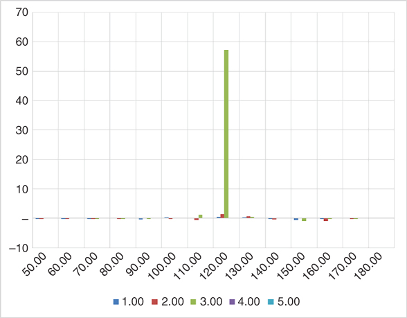
This is a good-quality superbucket, especially given it was obtained with simulations in just over a second. Superbuckets traditionally obtained with FDM are of similar quality and also take around a second to compute. Once again, we notice that AAD and parallelism bring FDM performance to Monte-Carlo simulations.

With the same settings (10 points spacing on the risk view), we compute the superbucket for a 2 years 105 call (first chart) and a 2.5 years 85 call (second chart). The results are displayed below. The calculation is proportionally faster for lower maturities, linearly in the total number of time steps. We see that vega is correctly interpolated over the risk view (with limited spilling that eventually disappears as we increase the number of paths and time steps).

Finally, with a maturity of 3 years, strike 120, and a (biweekly monitored) barrier of 150 (with a barrier smoothing of 1), we obtain the following. The calculation time is virtually unchanged, the barrier monitoring cost being essentially negligible.

This barrier superbucket has the typical, expected shape for an up-and-out call: positive vega concentrated at maturity on the strike, negative vega, also concentrated at maturity (with some spilling over the preceding maturity on the risk view from the interpolation), below the barrier, partly unwound by (perhaps counterintuitive but a systematic observation nonetheless) positive vega on the barrier.

Comparing with a bump risk for performance and correctness, we find that finite differences produce a very similar risk report in 45 around seconds. For a 3y maturity, it could be reduced to 30 seconds by only bumping active volatilities. We are computing “only” 42 risk sensitivities (14 strikes and 3 maturities up to 3y on the risk view), so AAD acceleration is less impressive here: times 30, probably down to times 20 with a smarter implementation of the bump risk.

However, in this particular case, AAD risk is also much more stable. The results of the bumped superbucket depend on the size of the bumps and the spacing of the local volatility and the risk view, in an unstable, explosive manner. It frequently produces results in the thousands in random cells where vega is expected in the tens. AAD superbuckets are resilient and stable, because derivatives are computed analytically, without ever actually changing the initial conditions.

Finally, the quality of the superbucket is dependent on how sparse is the risk view, and rapidly deteriorates when more strikes and maturities are added to it. This is a problem with superbuckets known in the industry: to obtain decent superbuckets over a thinly spaced risk view forces to increase the time steps at the expense of speed. It helps to implement simulation schemes more sophisticated than Euler's.

Iterative calibration

We mentioned that explicit, analytic calibration was an exceptional feature of Dupire's model. Other models are typically calibrated numerically. In general terms, calibration proceeds as follows. To calibrate the parameters of a model (say the local volatilities in a simulation model a la Dupire) to a market (say an IVS with a risk view ), pick instruments (say European calls of different strikes and maturities) and find the model parameters so that the model price of these instruments matches their market price.

Denote the market price of the instrument and its model price with parameters . The functions and are always explicit and generally analytic or quasi-analytic, depending on the nature of the market and model.

We call calibration error for instrument the quantity:

where is the weight of instrument in the calibration. Since and are explicit, it follows that is also explicit.

Calibration consists in finding the that minimizes the norm of . The optimal is a function of the market :

The minimization is conducted numerically, with an iterative procedure. Numerical Recipes [20] provides the code and explanations for many common optimization routines. The most commonly used in the financial industry is Levenberg and Marquardt's algorithm from their chapter 15.

It follows that is a function of , just like in the explicit case, but here this function is defined implicitly as the result of an iterative procedure.

Differentiation through calibration

As before, we compute a price in the calibrated model:

and assume that we effectively differentiated the valuation step so we know:

Our goal, as before, is to compute the market risks:

The difference is that is now an implicit function that involves a numerical fit, and it is not advisable to differentiate it directly, with AAD or otherwise.

First, numerical minimization is likely to take several seconds, which would not be RAM or cache efficient with AAD. Second, numerical minimization always involves control flow. AAD cannot differentiate control flow, and bumping through control flow is unstable. Finally, in case , the result is a best fit, not a perfect fit, and to blindly differentiate it could produce unstable sensitivities.

It follows that we compute the Jacobian of without actually differentiating , with a variant of the ancient Implicit Function Theorem, as described next. It also follows that check-pointing is no longer an option. We must compute the Jacobian of and calculate a matrix product to find . The matrix product must be calculated efficiently; we refer to our Chapter 1.

Note that although we cannot implement check-pointing in this case, we still want to separate the differentiation of from the differentiation of , because then we can compute efficiently with parallel, path-wise AAD

The Implicit Function Theorem

We want to compute the Jacobian without actually differentiating . Remember that:

and that:

is an explicit function that may be safely differentiated with AAD or otherwise.

To find as a function of the differentials of , we demonstrate a variant of the Implicit Function Theorem, or IFT.

The result of the calibration that realizes the minimum satisfies:

It follows that:

Differentiating with respect to , we get:

Assuming that the fit is “decent,” the errors at the optimum are negligible compared to the derivatives so we can drop the left term and get:

For clarity, we denote the derivative of with respect to its first variable , and its derivative to the second variable . Then, dropping the approximation in the equality:

And it follows that:

The Jacobian of the calibration, that is, the matrix of the derivatives of the calibrated model parameters to the market parameters, is the product of the pseudo-inverse of the differentials of the calibration errors to the model parameters, by the differentials of the errors to the market parameters.

The differentials and are computed by explicit differentiation, and the Jacobian of is computed with linear algebra without ever actually differentiating through the minimization. Finally, we have an expression for the market risks:

We call this formula the IFT. We note that this is the same formula as the well-known normal equation for a multidimensional linear regression:

The market risks correspond to the regression of the model risks of the transaction onto the market risks of the calibration instruments. When is square of full rank (the calibration is a unique perfect fit), that expression simplifies into:

In addition, in the case of a perfect fit, calibration weights are superfluous, hence:

and finally:

This formula further illustrates that we are projecting the model risks of the transaction onto the market risks of the calibration instruments. Note that in addition to dealing with weights, the complete IFT formula simply replaces the inverse in the simplified formula by a pseudo-inverse. It is best to use the complete IFT formula in all cases, the pseudo-inverse stabilizing results when approaches singularity.

We refer to [94] for an independent discussion of differentiation through calibration and application of the IFT.

We have derived two very different means of computing market risks out of model risks in this chapter: with the extremely efficient check-pointing technique when model parameters are explicitly derived from market parameters, and with the IFT formula when model parameters are calibrated to the market prices of a chosen set of instruments. These two methodologies combine to provide the means to separate the differentiation of the valuation, from the propagation of risks to market parameters. This separation is crucial, because it allows to differentiate valuation efficiently with parallel AAD in isolation, and then propagate the resulting derivative sensitivities to market variables with check-pointing when possible, or IFT otherwise.

Model hierarchies and risk propagation

We mentioned in Chapter 4 that linear markets, IVS, and dynamic models really form a hierarchy of models, where the parameters of a parent model are derived, or calibrated, from the parameters of its child models.

For instance, a one-factor Libor Market Model (LMM, [29]) is parameterized by a set of initial forward rates and a volatility matrix for these forward rates .

Neglecting Libor basis in the interest of simplicity, the initial rates are derived from the continuous discount curve on the linear rate market (LRM) by the explicit formula:

where is the duration of the forward rates, typically 3 or 6 months. The LRM constructs the discount curve by interpolation, which is a form of calibration, to a discrete set of par swap rates and other market-traded instruments. The reality of modern LRMs is much more complicated due to basis curves and collateral discounting, see [39], but they are still constructed by fitting parameters to a set of market instruments, hence, by calibration.

The LMM volatility surface is calibrated to an IVS , which, in this case, represents swaptions of strike , maturity into a swap of lifetime . This IVS itself typically calibrates to a discrete set of swaption-implied volatilities, where the corresponding forward swap rates are computed from the LRM's discount curve through the formula:

After the model is fully specified and calibrated, it may be applied to compute the value of a (perhaps exotic) transaction through (parallel) simulations.

This figure above illustrates the entire process for the valuation of a transaction, including calibrations. This figure is reminiscent of the DAGs of Chapter 9. The nodes here do not represent elementary mathematical operations, but successive transformations of parameters culminating into a valuation on the top node. Derivative sensitivities are propagated through this DAG, from model risks to market risks, in the exact same way that adjoints are propagated through a calculation DAG: in the reverse order from evaluation. AAD over (parallel) simulations results in derivatives to model parameters. From there, sensitivities to parameters propagate toward the leaves, applying IFT for traversing calibrations and check-pointing for traversing derivations. The risk propagation results in the desired market risks: derivatives to swap rates and swaption-implied volatilities.

Although we are not developing the code for the general risk propagation process (this is thousands of lines of code and the potential topic of a dedicated publication), we point out that this algorithm is at the core of a well-designed derivatives risk management system.