14.1 MULTIDIMENSIONAL DIFFERENTIATION

In this chapter, we discuss the efficient differentiation of multidimensional functions. In general terms, we have a function:

that produces results out of inputs . The function is implemented in code and we want to compute its Jacobian matrix:

as efficiently as possible.

We have seen that AAD run time is constant in , but linear in , and that this is the case even when the evaluation of is constant in , because the adjoint propagation step is always linear in . Finite differences, and most other differentiation algorithms, on the other hand, are constant in and linear in . As a result, AAD offers an order of magnitude acceleration in cases where the number of inputs is significantly larger than the number of results , as is typical in financial applications.

We have covered so far the case where , and AAD computes a large number of differentials very efficiently in constant time. When , linear time is inescapable. The time spent in the computation of the Jacobian matrix is necessarily:

The theoretical, asymptotic differentiation time will remain linear irrespective of our efforts. In situations of practical relevance, however, when is limited compared to , and the marginal cost is many times smaller than the fixed cost , the Jacobian computes in “almost” constant time. This is the best result we can hope to achieve.

In the context of financial simulations, we have efficiently differentiated one result in Chapter 12. We pointed out that this is not limited to the value of one transaction. Our library differentiates, for example, the value of a portfolio of many European options, defined as a single product on page 238. We can differentiate the value of a portfolio. What we cannot do is differentiate separately every transaction in the portfolio, and obtain an itemized risk report, one per transaction, as opposed to one aggregated risk report for the entire portfolio. The techniques in this chapter permit to compute itemized risk reports in “almost” the same time it takes to compute an aggregated one.

The reason why we deferred this discussion to the penultimate chapter is not difficulty. What we cover here is not especially hard if the previous chapters are well understood. We opted to explain the core mechanics of AAD in the context of a one-dimensional differentiation, in a focused manner and without the distraction of the notions and constructs necessary in the multidimensional case. In addition, one-dimensional differentiation, including the aggregated risk of a portfolio of transactions, constitutes by far the most common application in finance. For this reason, we take special care that the additional developments conducted here should not slow down the one-dimensional case.

14.2 TRADITIONAL MULTIDIMENSIONAL AAD

Traditional AAD does not provide specific support for multiple results in the AAD library, and leaves it to the client code to compute the Jacobian of in the following, rather self-evident, manner:

1. Evaluate an instrumented instance of , which builds its tape once and for all.
2. For each result :
   1. Reseed the tape, setting the adjoint of to one and all other adjoints on tape to zero.
   2. Back-propagate. Read the kth row of the Jacobian in the adjoints of the inputs . Store the results. Repeat.

Our code contains all the necessary pieces to implement this algorithm. The method:

on the Tape and Number classes reset the value of all adjoints on tape to zero. The method overloads:

on the Number class set the caller Number's adjoint to one prior to propagation.

The complexity of this algorithm is visibly linear in , back-propagation being repeated times. It may be efficient or not depending on the instrumented code. In the context of our simulation code, it is extremely inefficient.

To see this, remember that we optimized the simulation code of Chapter 6 so that as much calculation as possible happens once on initialization and as little as possible during the repeated simulations. The resulting tape, illustrated on page 414, is mainly populated with the model parameters and the initial computations, the simulation part occupying a minor fraction of the space. Consequently, we implemented in Chapter 12 a strong optimization whereby adjoints are back-propagated through the minor simulation piece repeatedly during simulations, and only once after all simulations completed, through the initialization phase.

It is this optimization, along with selective instrumentation, that allowed to differentiate simulations with remarkable speed, both against model parameters in Chapter 12 and against market variables in Chapter 13. But this is not scalable for a multidimensional differentiation. With the naive multidimensional AAD algorithm explained above, the adjoints of are reset after they are computed, so the adjoints of populate the tape next. We can no longer accumulate the adjoints of the parameters and initializers across simulations, because adjoints are overwritten by those of other results every time. To implement the traditional multidimensional algorithm would force us to repeatedly propagate adjoints, in every simulation, back to the beginning of the tape, resulting in a slower differentiation by orders of magnitude.

Traditional multidimensional AAD may be sufficient in some situations, but simulation is not one of them. We must find another way.

14.3 MULTIDIMENSIONAL ADJOINTS

After implementing and testing a number of possible solutions, we decided on a particularly efficient and rather simple one, although it cannot be implemented in client code without specific support from the AAD library: we work with not one, but multiple adjoints, one per result.

With the definitions and notations of Section 9.3, we define the instrumented calculation as a sequence of operations , that produce the intermediate results out of arguments where , being the set of indices of 's arguments in the sequence:

The first s are the inputs to the calculation: for , , and some s, typically late in the sequence, are the results:

Like in Section 9.3, we define the adjoints of all the intermediate results , except that adjoints are no longer scalars, but -dimensional vectors:

with .

To every operation number involved in the calculation, correspond not one adjoint , the derivative of the final result to the intermediate result , but adjoints, the derivatives of the final results to the intermediate result . This definition can be written in a compact, vector form:

It immediately follows this definition that:

so the desired Jacobian, the differentials of results to inputs, are still the input's adjoints. It also follows that for every component of :

which specifies the boundary condition for adjoint propagation. The adjoint equation itself immediately follows from the chain rule:

or, in compact vector form:

and the back-propagation equation from node to nodes follows:

or in compact form:

Unsurprisingly, this is the exact same equation as previously, only it is now a vector equation in dimension , no longer a scalar equation in dimension 1. The adjoints are propagated together from the adjoints , weighted by the same local derivative . It follows that back-propagation remains, as expected, linear in , but the rest is unchanged. For instance, in the case of simulations, we can propagate through a limited piece of the tape repeatedly during simulations, and through the initialization part, only once in the end. Therefore, the marginal cost of additional differentiated results remains limited, resulting in an “almost” constant time differentiation, as will be verified shortly with numerical results. First, we implement these equations in code.

14.4 AAD LIBRARY SUPPORT

The manipulations above cannot be directly implemented in client code. We must develop support in the AAD library for the representation, storage, and propagation of multidimensional adjoints. Those manipulations necessarily carry overhead, and we don't want to adversely affect the speed of one-dimensional differentiations. For this reason, and at the risk of code duplication, we keep the one-dimensional and multidimensional codes separate.

Static multidimensional indicators

First, we add some static indicators on the Node and Tape classes, that set the context to either single or multidimensional and specify its dimension. On the Node class, we add a static data member () that stores the dimension of adjoints, also the number of differentiated results. We keep it private, although it must be accessible from the Tape and Number classes, so we make these classes friends of the Node:

Similarly, we put a static boolean indicator on the Tape class. It is somewhat redundant with , although it is faster to test a boolean than compare a size_t to one. Since we test every time we record an operation, the performance gain justifies the duplication:

We also provide a function in AAD.h so client code may set the context prior to a differentiation:

This function returns a (unique) pointer on an RAII object that resets dimension to 1 on destruction:

Client code sets the context by a call like:

When exits scope for whatever reason, its destructor is invoked and the static context is reset to dimension one. This guarantees that the static context is always reset, even in the case of an exception, and that client code doesn't need to concern itself with the restoration of the context after completion.

The function and the RAII class must be declared friends to the Node and the Tape class to access the private indicators.

The Node class

The Node class is modified as follows:

In addition to the static indicator and friends discussed earlier, we have three modifications:

1. The storage of adjoints on line 14. We keep a scalar adjoint on the node for the one-dimensional case. In the multidimensional case, the adjoints live in separate memory on tape, like the derivatives and child adjoint pointers of Chapter 10, and are accessed with the pointer .
2. Consequently, we must modify how client code accesses adjoints on line 32. In the one-dimensional case, the single adjoint is accessed, as previously, with the accessor without arguments. In the multidimensional case, adjoints are accessed with an overload that takes the index of the adjoint between 0 and as an argument.
3. Finally, propagation on line 52 is unchanged in the one-dimensional case,¹ and we code another propagation function for the multidimensional case. This function back-propagates the adjoints altogether to the child adjoints, multiplied by the same local derivatives. Visual Studio 2017 vectorizes the innermost loop, another step on the way of an almost constant time differentiation.

The Tape class

The Tape class is modified in a similar manner:

1. We have an additional blocklist for the multidimensional adjoints on line 14.
2. The method performs, in the multidimensional case, the additional work following line 41: initialize the adjoints to zero, store them on the adjoint blocklist, and set the Node's pointer to access their memory space in the blocklist, like local derivatives and child adjoint pointers.
3. The method is upgraded to handle the multidimensional case with a global memset in the adjoint blocklist, line 60.
4. Finally, all the methods that clean, rewind, or mark the tape, like on line 76 or on line 85, are upgraded to also clean, rewind, or mark the adjoint blocklist so it is synchronized with the rest of the data on tape.

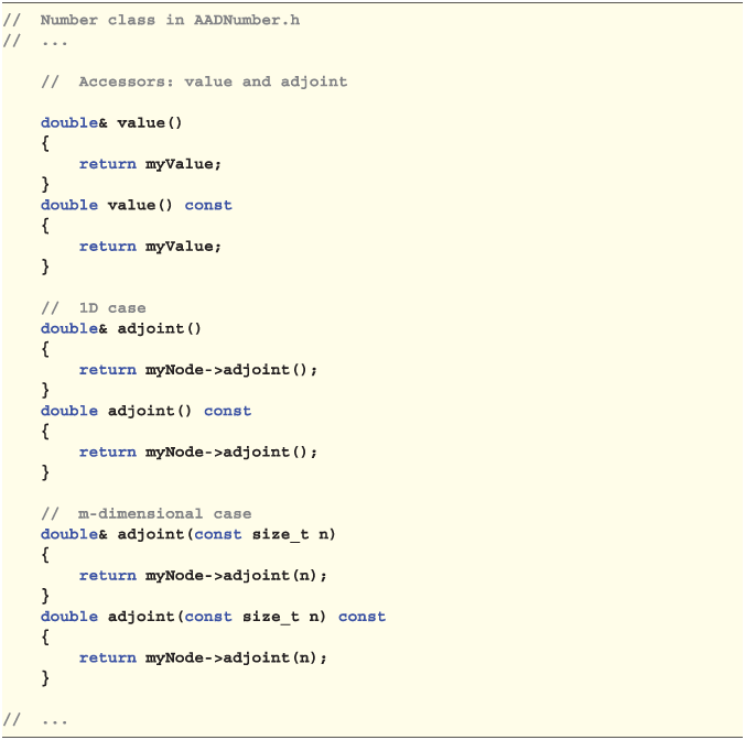
The Number class

Finally, we need some minor support in the Number class. First, we need some accessors for the multidimensional adjoints so client code may seed them before propagation and read them to pick differentials after propagation:

We also coded some methods to facilitate back-propagation on the Number type in Chapter 10. For multidimensional propagation, we only provide a general static method, leaving it to the client code to seed the tape and provide the correct start and end propagation points:

14.5 INSTRUMENTATION OF SIMULATION ALGORITHMS

With the correct instrumentation of the AAD library, we can easily develop the multidimensional counterparts of the template algorithms of Chapter 12 in mcBase.h. The code is mostly identical to the one-dimensional code, so the template codes could have been merged. We opted for duplication in the interest of clarity.

The nature of the results is different: we no longer return the vector of the risk sensitivities of one aggregate of the product's payoffs to the model parameters. We return the matrix of the risk sensitivities of all the product's payoffs to the model parameters:

The signature of the single-threaded and multi-threaded template algorithms is otherwise unchanged, with the exception that they no longer require a payoff aggregator from the client code, since they produce an itemized risk for all the payoffs. They are listed in mcBase.h, like the one-dimensional counterparts. The single-threaded template algorithm is listed below with differences to the one-dimensional version highlighted and commented:

The same modifications apply to the multi-threaded code, which is therefore listed below without highlighting or comments:

14.6 RESULTS

We need an entry-level function in main.h, almost identical to the and of Chapter 12:

so we can produce an itemized risk report. To produce numerical results, we set Dupire's model in the same way as for the numerical results of Chapter 12, where it took a second (half a second with the improvements in the next chapter) to produce the accurate microbucket of a barrier option of maturity 3y (with Sobol numbers, 500,000 paths over 156 weekly steps, in parallel over 8 cores). With a European call, without barrier monitoring, it takes around 850 ms (450 ms with expression templates).

To obtain the exact same microbucket for a single European call, but in a portfolio of one single transaction, with the multidimensional algorithm, takes 600 ms with expression templates. Irrespective of the number of itemized risk reports we are producing, multidimensional differentiation carries a measurable additional fixed overhead of around 30%. This is why we kept two separate cases instead of programming the one-dimensional case as multidimensional with dimension one.

To produce 50 microbuckets for 50 European options, with different strikes and maturity 3y or less, takes only 4,350 ms with expression templates, around seven times one microbucket. The following chart shows the times, in milliseconds, to produce itemized risk reports, with expression templates, as a function of the number of microbuckets:

As promised, the time is obviously linear in the number of transactions, but almost constant in the sense that the marginal time to produce an additional microbucket is only 80 ms, compared to the 600 ms for the production of one microbucket.

We produced 50 microbuckets in less than 5 seconds, but this is with the improvements of the next chapter. With the traditional AAD library, it takes around 15 seconds. The expression template optimization is particularly effective in this example, with an acceleration by a factor of three. Expression templates are introduced in the next and final chapter.