Chapter Five

 

 

Dynamic Linear Anti-windup Augmentation

5.1 OVERVIEW

In the previous chapter, linear static anti-windup designs inducing global and regional guarantees have been formulated and illustrated through several algorithms characterized by both full-authority and external architectures. It has been emphasized, however, that not all anti-windup problems admit such a simple compensation scheme.

Figure 5.1 Dynamic anti-windup compensation scheme.

Motivated by this fact, this chapter discusses a generalization of the linear static scheme wherein the matrix gains are replaced by a linear dynamic anti-windup compensator F with internal states. The static case will be recovered by this dynamic generalization when the size of the anti-windup filter state is zero. The interconnection of the dynamic anti-windup filter resembles that of the static case as shown in Figure 5.1. In particular, the filter is driven by the difference between the input and the output of the saturation nonlinearity, and the anti-windup filter outputs affect the unconstrained controller dynamics through signals that have access to the state and output equations of the unconstrained controller for the full-authority architecture or to the input and output signals of the unconstrained controller for the external architecture.

It should be emphasized that not only the dynamic generalization of the linear static schemes allows one to address and solve problems that cannot be solved using static techniques. Indeed, the extra degrees of freedom residing in a dynamic anti-windup compensation scheme allow, in general, to achieve increased performance levels therefore leading, in general, to improved responses as compared to those obtained with static anti-windup. The price to be paid for these advantages is the complexity of the anti-windup filter, which has an internal state whose dimension sums up with the dimension of the unconstrained controller when evaluating the computational complexity of the anti-windup augmented control system.

Similar to the static case, several algorithms will be given in this chapter for dynamic direct linear anti-windup (DLAW) compensation. In particular, first algorithms with global performance and stability guarantees will be given. These algorithms are prone to similar applicability limitations as their static counterpart, namely, they are only applicable to problems related to exponentially stable linear plants. These algorithms will be formulated using both the full-authority architecture and the external architecture. Next, an algorithm for plant-order anti-windup design will be given, which only induces regional guarantees on the closed loop but that is applicable to any type of windup-prone linear control system. All the algorithms are aimed at guaranteeing optimal (regional or global) input-output performance of the type discussed in Section 2.4.2.

Within the context of dynamic anti-windup, an important parameter is the order n_aw of the anti-windup filter. In this chapter, algorithms leading to compensators of the same order as the plant will be given first, because they are characterized by powerful feasibility conditions and convex formulations. Next, with the goal of reducing the complexity of the anti-windup compensators, algorithms for the design of reduced-order compensators will be given. These algorithms arise from approximate (convexified) solutions of nonconvex conditions, therefore they are not guaranteed to always provide a solution, but are often very effective for reduced-order anti-windup design.

5.2 KEY STATE-SPACE REPRESENTATIONS

Similar to the structure of Chapter 4, before introducing the anti-windup construction algorithms, it is useful to define some notation giving the equations for the plant and unconstrained controller under consideration and certain important matrices of the resulting closed loop.

The plant and unconstrained controller under consideration are the same as those in (4.1) and (4.2):

(5.1)

(5.2)

The general structure of the dynamic anti-windup compensator is described as follows, where, depending on the adopted architecture (full-authority or external), the correction signals v₁ and v₂

(5.3)

are injected at different locations in the unconstrained controller, as clarified next.

The dimension n_aw of the anti-windup state x_aw is a design parameter, and Λ_aw, B_aw, , and are matrices of appropriate dimensions that characterize the particular anti-windup solution adopted. In the special case where n_aw = 0, the size of the state x_aw is zero and the compensation scheme reduces to v₁ = D_aw,1 (u – sat(u)) and v₂ = D_aw2 (u – sat(u)), which corresponds to the static anti-windup scheme extensively discussed in the previous chapter.

The design approach for dynamic DLAW augmentation parallels that of the static DLAW augmentation. It is therefore necessary to rely on the same closed-loop representations that have been introduced and used in Section 4.2. They are reported next to make this chapter self-contained.

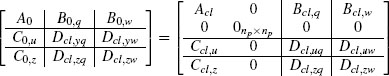
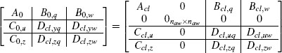
The compact closed-loop representation corresponds to the following system

(5.4)

which describes the closed loop before anti-windup augmentation with q = dz(u). The matrices in (5.4) are uniquely determined by the matrices in (5.1) and (5.2) and correspond to

(5.5a)

(5.5b)

where the matrices Δ_u := (I– D_c,yD_p,yu)^–1 and Δ_y := (I– D_p,yD_c,y)^–1 defined by the well-posedness of the unconstrained closed loop.

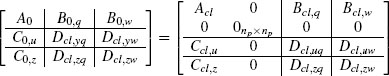
The closed-loop system (5.4) after anti-windup augmentation is equipped with an extra dynamical equation arising from the anti-windup compensator dynamics and by extra signals affecting the dynamics of the x_cl state variable:

(5.6)

where the matrices B_cl,v, D_cl,uv, and D_cl,zv depend on the architecture, full authority or external, of the compensation scheme under consideration The values of these matrices are detailed separately for the two architectures in the following two sections

5.2.1 Closed-loop representation with full-authority anti-windup

Full-authority dynamic linear anti-windup augmentation corresponds to modifying the controller equations (5.2) as follows:

(5.7)

where the two signals v₁ and v₂ are the two outputs of the anti-windup compensator (5.3).

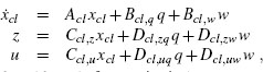
When adopting the full-authority architecture, the matrices B_c1,v, D_cl,u,v,and D_cl,zv in (5.6) correspond to the following values:

(5.8)

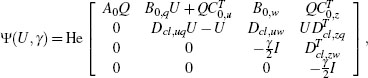
After designing the anti-windup compensator matrices using the full-authority algorithms reported in this chapter, the nonlinear performance of the resulting closed loop can be evaluated relying on the LMI-based tools introduced in Section 3.5.3 on page 66. To this end, the following equations will be useful to appropriately select the matrices in (3.54) to represent the dynamic full-authority linear anti-windup architecture with that notation:

(5.9)

where and Most of the examples provided in this chapter will incorporate a nonlinear L₂ gain analysis curve determined using transformation (5.9) and the tools of Section 3.5.3.

5.2.2 Closed-loop representation with external anti-windup

In the external anti-windup case, the modification signals denoted by v and enforced on the controller by the anti-windup compensator are not allowed to access all the controller states but can only affect the external signals, namely, the controller input and output. The controller equations (5.2) then become:

(5.10)

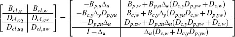
When adopting the external architecture, the matrices B_cl,v, D_cl,uv, and D_cl,zv in (5.6) correspond to the following values:

(5.11)

Similar to the full-authority case, external anti-windup schemes will also be analyzed by way of the nonlinear performance estimation tools of Section 3.5.3. To this end, the matrices in (3.54) should be selected using equation (5.9). However, for the external case, the matrices B_cl,v, D_cl,uv and D_cl,zv must be selected as in (5.11).

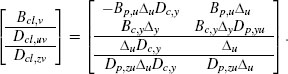
Paralleling the matrices given in Chapter 4, it is useful to introduce a last dynamical system called compact open-loop representation, which is described by the equations

(5.12)

where the input v₁ resembles the first signal injected by the external anti-windup action and where the matrices correspond to the following selections:

(5.13)

5.3 FACTORING RANK-DEFICIENT MATRICES

The goal of this section is to illustrate a simple mathematical tool which is required by the algorithms discussed in this chapter. In most cases, dynamic DLAW algorithms require an intermediate step where a symmetric rank-deficient matrix Ξ ∈ ^nxn of rank n_γ > n is factored as Ξ = NN^T, where N ∈ ^nxn is a rectangular matrix having full column rank. The next procedure allows one to construct one of the infinitely many solutions to the above mentioned factorization.

Procedure 1 (Factorization of a rank-deficient matrix)

Step a) Define the symmetric matrix Ξ ∈ ^nxn having rank nξ > n.

Step b) Compute the singular value decomposition of Ξ, namely, a diagonal matrix S_> having nonnegative diagonal entries with the last n-n_ξ diagonal entries equal to zero, and a square matrix U_ξ such that Ξ = U_ξS_ξU_ξ^T. Numerically this can be done using, for example, the MATLAB command [U, S, V] = SVD(X_i), which returns U=V whenever its argument is symmetric.

Step c) Define as the matrix having the first columns of U_ξ and define as the upper left n _ξ× n _ξ square 0 block of the matrix S_ξ. Since only the first n_ξ diagonal entries of S_ξare nonzero, then

Step d) Define as diagonal matrix having on its diagonal the square roots of the diagonal terms of so that . Numerically this can be done using, for example, the MATLAB command sqS = sqrtm(S). Select

(5.2)

and note that N ∈ ^n_ξ×n and that as desired.

5.4 ALGORITHMS PROVIDING GLOBAL GUARANTEES

In this section constructive techniques for the selection of the dynamic anti-windup compensator matrices in (5.3) are given, with the goal of guaranteeing global guarantees on the internal stability and input-output gain of the resulting closed-loop system. This section should be then understood as the dynamic counterpart of the previous Section 4.3 related to static DLAW. Similar to the static case, exponential stability of the plant is a necessary condition for dynamic DLAW with global guarantees to be applicable, while to deal with non-exponentially stable plants the reader should refer to the regional algorithms reported in the subsequent Section 5.5. An appealing result that characterizes the dynamic DLAW techniques is that whenever the plant is exponentially stable, there always exists a dynamic anti-windup compensator of the same order as the plant that solves the global problem. Therefore, dynamic anti-windup compensation constitutes a step forward as compared to static compensation techniques, where suitable feasibility conditions were required to hold for the algorithms to be applicable.

5.4.1 Global full-authority plant-order augmentation

Full-authority linear dynamic anti-windup compensation synthesis amounts to selecting the matrices (Λ_aw, B_aw, C_aw,1, D_aw,1, C_aw,2, D_aw,2) of the anti-windup compensator (5.3) corresponding to the block F in Figure 5.1 when the signal v acts both on the state and on the output equations of the unconstrained controller. An algorithm to construct a plant-order version of such a full-authority anti-windup compensation is offered in this section. Reduced-order design will be addressed in the following section.

Algorithm 4 (Dynamic plant-order full-authority global DLAW)

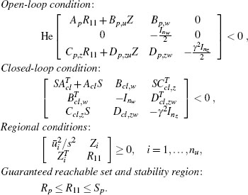
Step 1. Given a plant and a controller of the form (5.1), (5.2), construct the matrices of the compact closed-loop representation using (5.5) and (5.8). Select a constant v ∈ [0,1) used to enforce a strong well-posedness constraint (see Section 3.4.2 on page 60).

Step 2. Find the optimal solution (R₁₁, S, γ) ∈ ^np×np × ^n_cl×n_cl × to the following LMI eigenvalue problem which is always feasible for exponentially stable plants:

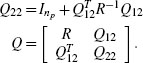
Step 3. Based on the solution determined at the previous step, construct the symmetric matrix and define Q₁₂ ∈ ^ncl×np as any solution to the following equation:

(5.14)

which is always solvable and admits infinitely many solutions because by construction, rank(RS⁻¹R − R) = rank((RS⁻¹R − R)(R⁻¹S))= rank(R −S) = n_aw. A solution can be determined following Procedure 1 on page 113 with Ξ = RS⁻¹R −R. Then define the following matrices:

Step 4. Based on the matrices determined at steps 1 and 3, define the following matrices (where the second row and column of zeros have size n_p):

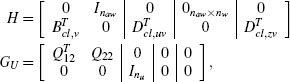
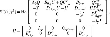
and construct the matrices G _U ∈ ^(np+nu)×m, H ∈ ^{m×(n_p+n_c+n_u)}, and Ψ ∈ ^m×m, with m := n_cl + n_p + n_u + n_w + n_z, as follows:

where for any square matrix X, He(X) = X + X^T.

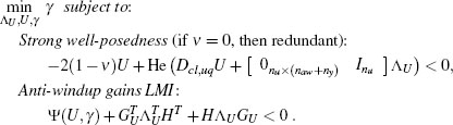
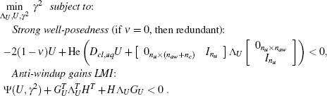
Step 5. Find the optimal solution (∧_U,U,γ) of the LMI eigenvalue problem:

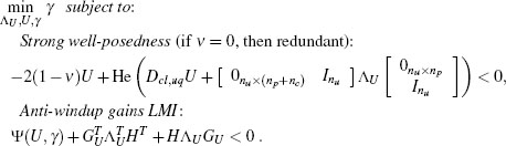
Step 6. Select the plant-order full-authority anti-windup compensator as:

with the selection

5.4.1.1 Case studies

The plant-order DLAW construction of Algorithm 4 will be now applied to the five examples used in Chapter 4 to illustrate global static DLAW designs. Since all of these examples are characterized by exponentially stable plants, plant-order anti-windup will be applicable to all of them. In some cases, the resulting scheme will lead to improved performance as compared to that induced by the static compensators. In some other cases, dynamic anti-windup will be mandatory because the static approach was not feasible. However, for a few of those examples, it will be evident that dynamic anti-windup leads to comparable responses to those obtained with the static compensation architecture. For these examples it will not be worth the extra computational effort required to implement a dynamic DLAW scheme and the static one will be the preferred solution.

The first example is the MIMO academic example no. 2. For this example, plant-order full-authority anti-windup behaves no better than the static anti-windup results illustrated in Example 4.3.2 for the static full-authority DLAW case and in Example 4.3.6 for the static external DLAW case.

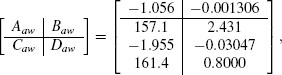
Example 5.4.1 (MIMO academic example no. 2) Consider the MIMO academic example whose data is given in Example 4.3.2 on page 85. Constructing a plant-order anti-windup compensator is of no use as highlighted above, but it is instructive to focus on the use of Algorithm 4 and the use of tricks to reduce the size of the resulting matrices, as discussed in Section 3.7.2. Indeed, when running Algorithm 4 as is, the achievable performance is γ = 1.55, which is roughly the same as what can be obtained with static anti-windup. However, the size of the entries in the anti-windup matrices obtained at step 6 are roughly 10⁶ due to some numerical issue with the LMI optimizer. More specifically, the matrices obtained are:

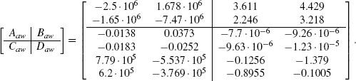
The resulting simulation is unacceptably slow and reveals the unsuitability of this compensator. The numerical problem is easily solved by following the steps outlined in Section 3.7.2. In particular, the following two inequalities are added to the LMIs at step 5:

(5.15)

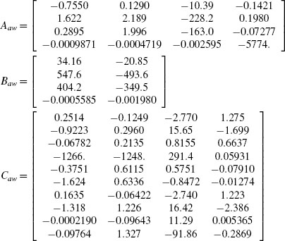
with κ = 10 (note that choosing κ too small will result in infeasibility of the LMIs at step 5). The resulting compensator induces a performance level γ =1.56 (slightly deteriorated) but the anti-windup compensator matrices become

much more reasonable from a numerical viewpoint. As anticipated above, the simulation results and the nonlinear L₂ gain curve obtained from this plant-order compensator coincide with the static anti-windup solution of Example 4.3.2; therefore the static solution is preferred to this one due to its simpler architecture.

The next example is the passive electrical circuit introduced in Example 4.3.3 and revisited in Example 4.3.7. For this example, the extra degrees of freedom available in the plant-order anti-windup scheme lead to improved performance and improved closed-loop responses.

Example 5.4.2 (Electrical network) Consider the electrical network studied in Examples 4.3.3 and 4.4.3 and represented in Figure 4.6 on page 87 of the previous chapter.

For this example the global guarantees given by the static Algorithm 1 in Example 4.3.3 come at the price of a sluggish response (see Figure 4.3.3 on page 87). When moving into dynamic plant-order anti-windup, the response is much improved and the global guarantees are still at hand. Indeed, by selecting the parameters v = 0.01 and imposing the extra bound (5.15) with κ = 1000 on the size of the anti-windup matrices, Algorithm 4, provides the following anti-windup compensator:

which guarantees a global L₂ performance level θ = 58.428 (much improved as compared to the value 85. 22 obtained with static compensation). With this anti-windup compensator, the closed-loop response corresponds to the curves of Figure 5.2 where a significant improvement can be appreciated as compared to the static responses of Example 4.3.3.

Figure 5.2 Plant output and input responses of various closed loops for Example 5.4.2.

It should be emphasized that an even more desirable response had been ob tained when using regional static anti-windup compensation in Example 4.4.3 on page 105. However, the regional compensation did not provide guaranteed global L₂ gain and the resulting global exponential stability property. This is guaranteed instead by the (possibly more conservative) compensation resulting from Algorithm 4.

Figure 5.3 Nonlinear gains for Examples 4.3.3 and 5.4.2 characterizing the system before and after static and plant-order anti-windup augmentation.

Figure 5.3 shows the nonlinear gain curves corresponding to no anti-windup (dotted), static anti-windup (dashed), and plant-order anti-windup (solid). Clearly, the global L₂ gain obtained from plant-order anti-windup is improved as compared to the static condition because the optimizer has extra degrees of freedom. For this example, the whole L₂ gain curve associated with plant-order compensation is improved as compared to the static one. Therefore, improved responses on all signal ranges are to be expected (within the limits of the conservativeness of the quadratic L₂ performance bound).

The following example has been introduced in Example 4.3.4 where it was shown that static anti-windup design is not feasible (using either the full-authority or the external architecture). Plant-order anti-windup is feasible and provides a desirable solution to this windup problem.

Example 5.4.3 (SISO academic example no. 2) Consider the SISO closed-loop system described in Example 4.3.4 on page 89. It was illustrated in that example that static anti-windup with global guarantees is not feasible. Conversely, Algorithm 4 always provides a feasible solution as long as the plant is exponentially stable and applying the algorithm with v = 0.5 and limiting the anti-windup matrices as in Example 5.4.1 (see equation (5.15)) with κ = 5, the following plant-order compensator is obtained:

which guarantees a global L₂ gain γ = 4.466 and gives the desirable response represented in Figure 5.4.

Figure 5.4 Plant output and input responses of various closed loops for Example 5.4.3.

Note that the anti-windup response of Figure 5.4 is pretty comparable to that one obtained using regional static anti-windup compensation as illustrated in Example 4.4.2 and in Figure 4.16 on page 105. However, the regional static design appears to be more aggressive than the global dynamic one, which is reasonable based on the fact that the aggressive regional design is not associated with any global asymptotic stability guarantee, while the less aggressive global one guarantees closed-loop global exponential stability.

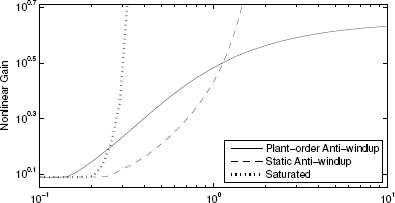
Figure 5.5 Nonlinear gains for Examples 4.4.2 and 5.4.3 characterizing the system before and after regional static and global plant-order anti-windup augmentation.

This fact is especially evident in Figure 5.5, where three nonlinear gains are compared to each other. The dotted curve represents the closed loop without anti windup, the dashed one is the static regional anti-windup curve of Example 4.4.2 (see also Figure 4.17 on page 105), which enlarges the guaranteed stability region but still doesn't provide global properties, and the solid one is the plant-order anti-windup curve using the compensation described here. It is quite interesting also the fact that the nonlinear gains behavior for small signals suggests that the closed loop with plant-order anti-windup performs worse than no anti-windup. This is consistent with simulations involving smaller step references (r = 0.2) than that of Figure 5.4, where the saturated response appears closer to the unconstrained one.

In the next example, the longitudinal dynamics of an F8 aircraft introduced in Section 1.2.3 and revisited in Example 4.3.5 on page 90 is considered. In particular, for this system it is shown here that plant-order full-authority anti-windup can compensate for the unpleasant bias experienced in Example 4.3.5 when using static compensation.

Example 5.4.4(F8 longitudinal dynamics) Consider the problem statement formally described and introduced in Example 4.3.5 on page 90. It was shown in that example (see in particular the simulations of Figure 4.9 on page 91) that static anti-windup could only lead to a partial solution of the windup problem. Indeed, in that simulation the anti-windup response exhibited a very slow convergence to the desired output value. It was also noted in Example 4.3.8 on page 97 later in that same chapter that external static anti-windup is not feasible for this study case.

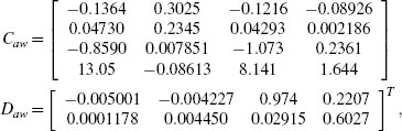
When using plant-order anti-windup compensation, this problem can be overcome. In particular, by running Algorithm 4 with the same exact parameters as in Example 4.3.5 and enforcing the extra constraint (5.15) on the anti-windup compensator size with κ = 8000, the following anti-windup compensator is obtained:

This compensator achieves global performance level γ = 25.476, clearly improved with respect to the one achievable by static anti-windup in Example 4.3.5, which was γ = 26.44.

Figure 5.6 Plant output responses of various closed loops for Example 5.4.4.

Figure 5.6 represents the output response of the system with plant-order compensation. This should be compared to Figure 4.9 on page 91 representing the same response using static anti-windup. The new simulation is much improved because the slow convergence has been significantly suppressed by the new dynamic anti-windup solution. This increased quality of the dynamic anti-windup response is also confirmed by the comparison of the nonlinear L₂ gain curves in Figure 5.7 where the plant-order solution (solid curve) lies below the static solution (dashed curve) on the whole disturbance input size range.

5.4.2 Global full-authority reduced-order augmentation

In Sections 4.3.1 and 5.4.1, respectively, design algorithms for static and plant-order full-authority DLAW augmentation with global guarantees have been given.

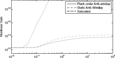
Figure 5.7 Nonlinear gains for Example 5.4.4 characterizing the system before (dotted) and after static (dashed) and plant-order (solid) anti-windup augmentation.

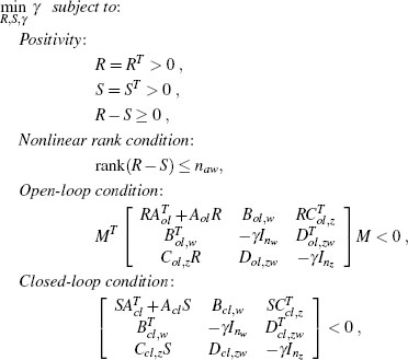
In particular, the construction procedures correspond to Algorithms 1 and 4, respectively. Is has also been emphasized that plant-order DLAW augmentation is always feasible for exponentially stable plants, whereas static augmentation is only possible provided certain feasibility conditions are satisfied by the problem data. It turns out that, as suggested by their similarity, both the abovementioned algorithms are special cases of a general result of linear full-authority anti-windup augmentation where the order of the compensator is any positive integer n_aw However, for generic values of n_aw, the corresponding anti-windup construction cannot be formulated in terms of LMIs, as it is the case for Algorithms 1 and 4, and the corresponding anti-windup design becomes more complex. For a fixed anti-windup compensator order n_aw (with n_aw = 0 and n_aw ≠ n_p), what makes the generalized algorithm difficult to solve is determining the solution R, S, γ at the first optimization step. All the remaining steps are roughly unchanged. The first optimization step generalizes the LMI optimization problem at step 3 of Algorithm 1 and the LMI optimization problem at step 2 of Algorithm 4. Given any integer value n_aw ≥ 0, this generalization can be written as follows:

(5.16)

The crucial constraint in the optimization problem (5.16) is the nonlinear rank constraint, rank(R₁₁ − S₁₁) ≤ n_aw. It is easy to verify that for n_aw = 0 (static anti-windup), the constraint corresponds to requiring R = S, and (5.16) becomes linear and reduces to the LMI optimization reported at step 3 of Algorithm 1. Similarly, if n_aw ≥ n_p, the nonlinear rank condition is automatically implied by the fact that the rank of the matrix R₁₁− S₁₁ cannot be larger than its size n_p. For any other selection of n_aw>0, the problem (5.16) remains nonlinear and hard to solve.

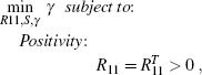
Understanding the problem behind the optimization problem (5.16), however, allows one to introduce a new design tool which is useful whenever full-authority static anti-windup augmentation is not feasible or leads to unsatisfactory performance. In this case, it is of interest to look for “reduced-order” anti-windup augmentation with a certain performance guarantee y_G, namely, to search for a minimized value of n_aw such that the constraints (5.16) have a solution with y = y_G. The reduced-order DLAW problem can be addressed through an approximate approach arising from the observation that since R₁₁ − S₁₁ ≥ 0, the trace of R₁₁ − S₁₁(namely, the sum of all the diagonal entries of R₁₁ − S₁₁) is proportional to the size of R − S. Therefore, minimizing the trace of R₁₁ − S₁₁ leads, in general, to a rank-deficient result whose rank will be the order of the anti-windup compensator. The optimization problem (5.16) can then be solved by removing the nonlinear rank constraint, replacing γ by the constant γ_G and minimizing the new cost variable trace(R₁₁ − S₁₁). The value γ_G can be selected as αγ_np, where γ_np is the achievable gain by plant-order anti-windup augmentation and α > 1 is a constant parameter quantifying how much performance the designer is willing to give up to reduce the dimension n_aw of the anti-windup compensator matrices. Note, however, that the final rank-deficient solution may need to give up a little on the pre-assigned guaranteed performance level γ_G because a suitable correction on S₁₁ is required to make R₁₁ − S₁₁ a rank-deficient matrix.

In the numerical implementation of this direct linear anti-windup algorithm, the constraint R₁₁ − S₁₁ ≥ 0 will actually be replaced by the strict inequality constraint R₁₁ − S₁₁ > 0, and the solution R₁₁ − S₁₁ will be very close to being rank deficient. Therefore, it will be useful to use singular value decomposition (SVD) to determine a new selection of S for which R₁₁ − S₁₁ > 0 actually holds. Since the S matrix is slightly changed by this modification, it is mandatory to verify that the new selection of S still satisfies the closed-loop condition in (5.16). To this end, anticipating for such a perturbation, it is useful to add a small feasibility margin to the open closed-loop condition to make it robust to these perturbations (at least to a certain extent). The resulting constraint will be

where ε > 0 is a small constant. The complete procedure for the selection R₁₁, S, γ characterizing a minimal order anti-windup compensator requires some tuning for ε and γ_G but is typically quite straightforward to apply. The main steps of the procedure are reported next.

Procedure 2 (Computation of an (R, S, γ) solution for reduced-order full-authority anti-windup with guaranteed performance)

Step a) A plant and a controller of the form (5.1), (5.2) and the matrices of the compact closed-loop representation constructed based on equations (5.5) and (5.8) are given. A small positive constant ε to robustify the closed-loop LMI condition and a value y_G characterizing the desired guaranteed performance are also given. Note that the actual performance y* achieved by the minimal-order (R, S, y) solution will be, in general, larger than y_G but often very close to it.

Step b) Find the optimal solution (R₁₁, S ∈ ^n_p×n_p×^n_cl×n_cl to the following LMI eigenvalue problem:

Step c) Compute the SVD of the symmetric matrix R₁₁−S₁₁ determined from the solution of the previous step, namely, compute F, Λ such that F Λ F^T = R ₁₁ −S₁₁ where Λ is a positive semidefinite diagonal matrix whose diagonal entries are nonincreasing (for example, use the MATLAB command [U,Lambda,V] = svd(R11-Sll) ; F = (U+V)/2;). Set n_aw = n_p

Step d) Call λ₁,…. λ_naw-1 the first n_aw – 1 entries on the diagonal of Λ and define namely, is a diagonal matrix having its first “_aw – 1 diagonal entries equal to the entries of Λ and the remaining entries equal to zero. Also define

Step e) Given the matrix , where ₁₁ was determined at the previous step, verify the feasibility of the following LMI in the free variable γ

If the LMI is feasible, then set (R₁₁^*, S^*,γ*) := (R₁₁, Ŝ, γ) set n_aw = n_aw – 1, and go to step d. If the LMI is not feasible, then go to step f.

Step f) Select the order of the anti-windup compensator as n_aw and the (R, S, γ) solution as (R₁₁^*, S^*,γ*).

The performance level induced by the reduced-order anti-windup compensator is in general larger (namely, worse) than the performance γ_np induced by the plant-order anti-windup design. This is true because of two reasons: first, the guaranteed performance γ_G will have to be larger than γ_np, in general, to allow for satisfactory reductions of n_aw ; second, due to the fact that the matrix Ŝ defined at step 5 is different from the original matrix S, the optimization at that same step might lead to a slightly deteriorated performance level. It has, however, been noted in several case studies that the value of γ^* is not too different from γ_G.

Once a triple (R^*₁₁, S^*,γ*) satisfying (5.16) with a small enough n_aw is determined from Procedure 2, the reduced-order anti-windup construction can be carried out following a simple generalization of the previous Algorithms 1 and 4, which is reported next.

Algorithm 5 (Dynamic reduced-order full-authority global DLAW)

Step 1. Given a plant and a controller of the form (5.1), (5.2), construct the matrices of the compact closed-loop representation using (5.5) and (5.8). Select a small positive constant ε to robustify the order minimization procedure and a constant α > 1 characterizing the amount of performance to be traded in for order reduction. Select a constant v ∈ [0,1) used to enforce a strong well-posedness constraint (see Section 3.4.2 on page 60).

Step 2. Find the optimal solution (R₁₁, S, γ_np) ∈ ^n_p×n_p × ^n_cl×n_cl × to the following LMI eigenvalue problem which is always feasible for exponentially stable plants:

The resulting performance level γ_np corresponds to the maximum performance achievable by plant-order anti-windup augmentation.

Step 3. Based on the matrices and parameters determined at step 1, select the desired guaranteed performance as γ_G = αγ_np and determine the reduced compensator order n_aw and the triple from Procedure 2.

Step 4. Based on the solution determined at the previous step, construct the symmetric matrix , and define Q₁₂ ∈ ^n_cl×n_aw as any solution to the following equation:

which is always solvable and admits infinitely many solutions because by construction rank(RS^-1R − R) = rank((RS^-1R − R)(R^-1S)) = rank(R - S) = n_aw. A solution can be determined following Procedure 1 on page 113 with Ξ = R−S⁻¹R − R. Then define the following matrices:

Step 5. Based on the matrices determined at steps 1 and 4, define the following matrices (where the second row and column of zeros have size naw):

and construct the matrices G_U ∈ ^{(n_aw+n_u)×m}, H ∈ ^{m×(n_aw+n_c+n_u)}, and Ψ ∈ ^m×m, with m := n_cl + n_aw + n_u + n_w + n_z, as follows:

where for any square matrix X, He(X) = X + X^T

Step 6. Find the optimal solution (Λ_u, U,γ) of the LMI eigenvalue problem:

Step 7. Select the plant-order full-authority anti-windup compensator as:

with the selection .

Since the above reduced-order DLAW algorithm aims at reducing as much as possible the size of the anti-windup compensator state (while giving global stability and performance guarantees), its use is recommended in cases where the static anti-windup design of Algorithm 1 is not feasible or leads to unsatisfactory performance. Indeed, whenever Algorithm 1 is applicable, in the best case the reduced-order augmentation algorithm will lead to the same result, even though it will get there by a more complex route and, due to the approximate nature of the approach, it is not even guaranteed to provide the same level of performance. This is illustrated next in an example reconsidering the problem statement in Example 4.3.4 for which static full-authority anti-windup had been shown to be in-feasible in Section 4.3.1. For this example, Algorithm 5 leads to a reduced-order linear anti-windup filter.

Example 5.4.5 (SISO academic example no. 2) Consider the problem statement in Example 4.3.4 (on page 89) where no static full-authority anti-windup with global guarantees can be determined. That anti-windup problem has been revisited twice already: in Example 4.4.2 (on page 104) where a regional static anti-windup had been synthesized and in Example 5.4.3 (on page 119), where global plant-order anti-windup had been designed.

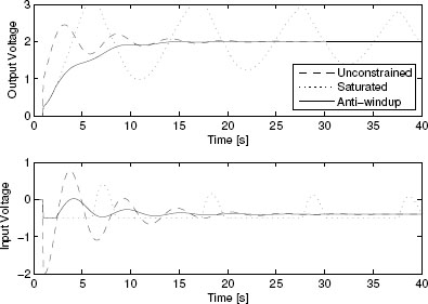
Figure 5.8 Plant output and input responses of various closed loops for Example 5.4.5.

The example is here revisited by running Algorithm 5 to obtain a reduced (or minimum)-order anti-windup guaranteeing a global performance almost as good as the global performance γ = 4.466 induced by the plant-order solution of Example 5.4.3. In particular, by choosing to give up by seventy percent on that global performance and selecting γ_G = 1.7.4.466 = 7.6 and ε = 10⁻⁴ in Procedure 2, a first-order compensator can be obtained guaranteeing a closed-loop performance γ* = 7.57. The compensator matrices are obtained by following all the steps of Algorithm 5 as

To this end, no constraints have been enforced on the anti-windup matrices sizes and the parameter v has been selected as v = 0. 1.

Figure 5.8 represents the closed-loop responses of the saturated (dotted), unconstrained (dashed), and anti-windup (solid) closed loops. From comparing the plots to the other responses in the previous Examples 4.4.2 and 5.4.3, it appears that this reduced-order design provides a comparable type of response thus successfully solving the windup problem.

It is also instructive to inspect Figure 5.9 where the nonlinear L₂ gains corresponding to the saturated closed loop (dotted) and to the various anti-windup closed loops synthesized in the previous Examples 4.4.2, 5.4.3 and in this one are compared. It appears from these curves that the reduced-order solution (solid) is expected to pretty much behave in the same way as the plant-order solution. Notice that in this case the nonlinear gain obtained from the reduced-order solution even improves upon the plant-order one on a wide range of input sizes. It is emphasized that the optimizers in all the algorithms providing global guarantees operate by only looking at the global L₂ gain (namely, the far right of the nonlinear L₂ gain curve) and therefore there is no a priori guarantee that one approach or the other will give better curves for values of the input size smaller than infinity.¹

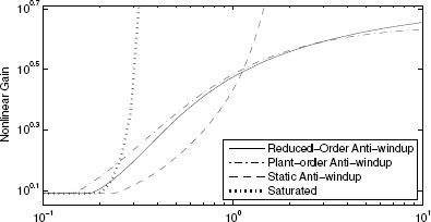
Figure 5.9 Nonlinear gains for Examples 4.4.2, 5.4.3, and 5.4.5 characterizing the system before (dotted) and after regional static (dashed), global plant-order (dashed-dotted), and global reduced-order (solid) anti-windup augmentation.

5.4.3 Global external plant-order augmentation

Paralleling the static case discussed in the previous chapter, external dynamic anti-windup compensation synthesis addresses the selection of the anti-windup compensator matrices (Λ_aw, B_aw,C_aw, and D_aw) when using the external architecture represented in Figure 5.10 where F represents the anti-windup compensator. In this and the following section, external anti-windup design algorithms will be given paralleling the full-authority approaches commented on in the previous sections.

When the anti-windup compensator order is equal to the size of the plant state, the algorithm provided here is always feasible for loops involving exponentially stable plants, thus overcoming certain limitations of the static external anti-windup approach of Algorithm 2 given on page 94.

Algorithm 6 (Dynamic plant-order external global DLAW)

Figure 5.10 External anti-windup compensation scheme.

Step 1. Given a plant and a controller of the form (5.1), (5.2), construct the matrices of the compact closed-loop representation using (5.5) and (5.11). Select a constant v ∈ [0,1) used to enforce a strong well-posedness constraint (see Section 3.4.2 on page 60). Moreover, based on the matrix B_{o1,v ⊥} in equation (5.13) generate any matrix B_{ol,v ⊥} that spans the null space of its transpose, namely such that B^T_ol,v⊥ B_ol,v⊥ = 0 and such that rank(B_{ol,v ⊥}) + rank(B_o1,v) = nc + np. (Note that in general there can be infinite selections of B_{ol,v ⊥}. As an example, using MATLAB, an orthonormal selection of B_ol,v⊥ is easily computed using Bolperp = null(Bolv).)

Step 2. Define 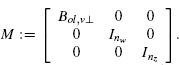Based on the matrices determined at step 1, find the optimal solution (R, S, γ)∈^{n_cl×xn_cl× n_cl×xn_cl×}× of the following eigenvalue problem which is always feasible for exponentially stable plants:

Step 3. Based on the solution determined at the previous step, define Q₁₂ ∈ ^{n_cl× n_p} as any solution to the following equation:

which is always solvable and admits infinitely many solutions because by construction, rank(RS⁻¹ R − R) = rank((RS⁻¹R − R)(R⁻¹S)) = rank(R − S) = n_p. A solution can be determined following Procedure 1 on page 113 with Ξ = RS⁻¹R − R. Then define the following matrices:

Step 4. Based on the matrices determined at steps 1 and 3 define the following matrices (where the second row and column of zeros has size n_p):

and construct the matrices G _U ∈ ^(np+nu)×m, H ∈ ^{m×(n_p+n_c+n_u)}, and Ψ ∈ ^m×m, with m := n_cl + n_p + n_u + n_w + n_z, as follows:

where for any square matrix X, He(X) = X + X^T.

Step 5. Find the optimal solution (Λ_u, U, γ) of the LMI eigenvalue problem:

Step 6. Select the plant-order external anti-windup compensator as:

with the selection

Example 5.4.6 (Electrical network) Consider again the electrical network problem studied in Examples 4.3.3 and 4.4.3 of the previous chapter and revisited in Example 5.4.2 of this chapter.

For this example, the full-authority plant-order anti-windup in Example 5.4.2 already showed an improvement compared to the static solutions of the previous chapter. Using external compensation allows practically the same performance to be achieved but with a simpler architecture. In particular, following Algorithm 6 and selecting the same parameters as those of the full-authority case in Example 5.4.2 (namely, v = 0.01 and k = 1000), the following compensator is determined:

which induces the global L₂ gain γ = 58.7 (almost the same as the gain γ = 58.428 induced by the full-authority solution of Example 5.4.2). Moreover, the simulation responses and the nonlinear L₂ gain curve achieved using this external anti-windup compensator are perfectly matched to those ones achieved using the full-authority one and reported in Figures 5.2 and 5.3. For this example, external anti-windup is therefore more desirable than full-authority anti-windup because of its simpler architecture for an identical performance.

In contrast to the above example, in the next example it is evident that the lesser degrees of freedom available to external anti-windup design lead to a solution which is not as desirable as the one obtained using the full-authority design.

Example 5.4.7 (F8 longitudinal dynamics) Consider the problem statement formally described and introduced in Example 4.3.5 on page 90. This example has been revisited a few pages earlier as Example 5.4.4 on page 121. In particular, it was shown in this last example that full-authority plant-order anti-windup is able to overcome some undesirable slow convergence experienced with static full-authority anti-windup in Example 4.3.5 (compare Figure 4.9 on page 91 with Figure 5.6 on page 122).

For this same case study, it was also discussed in Example 4.3.8 on page 97 that external static anti-windup is not feasible. Thus, already with static anti-windup designs, the extra degrees of freedom available to full-authority design in this case do make a difference in the feasibility conditions and on the achievable performance. This is further illustrated here, where it is shown that external plant-order anti-windup is feasible but the performance that it leads to is not as good as the one obtained from the full-authority design. When running Algorithm 6 for this problem statement (also condition (5.15) on the anti-windup compensator size is used, with k = 100, but this doesn't impact the achievable performance), the achievable closed-loop performance is γ = 51.18, highly deteriorated as compared to the γ = 25.476 achieved by full-authority compensation.

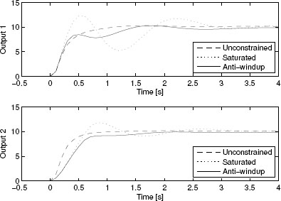
Figure 5.11 Plant output responses of various closed loops for Example 5.4.7.

The anti-windup compensator matrices are the following:

Figure 5.12 Nonlinear gains for Example 5.4.7 characterizing the system before (dotted) and after static full-authority (dashed), plant-order full-authority (dashed-dotted), and plant-order external anti-windup augmentation.

clearly less computationally intensive than the full-authority matrices in Example 5.4.4. However, the increased simplicity of the anti-windup architecture comes at the cost of a deteriorated output response. Figure 5.11 shows this response which should be compared to the more desirable response in Figure 5.6 on page 122.

This performance deterioration is also confirmed by the comparison of the nonlinear L₂ gain curves, which is reported in Figure 5.12. In particular, in Figure 5.12 four nonlinear L₂ gains are compared to each other: the saturated system without anti-windup (dotted), the system with the static full-authority anti-windup compensation of Example 4.3.5 (dashed), the plant-order full-authority anti-windup compensation of Example 5.4.4 (dashed-dotted), and the plant-order external compensation of this example (solid). Surprisingly, external dynamic compensation is not even able to do better than static full-authority compensation (the solid curve is all above the dashed curve), which means that the extra control directions available to the full-authority compensation are even more useful than having the extra dynamics available to the external plant-order approach. Indeed, the performance comparison suggested by the curves in Figure 5.12 is in agreement with the output responses experienced in Figures 4.9, 5.6, and 5.11 which refer to the three Examples 4.3.5, 5.4.4, and 5.4.7 under consideration.

5.4.4 Global external reduced-order augmentation

Similar to the full-authority construction introduced in Section 5.4.2 on page 122, reduced-order external anti-windup can also be achieved by suitably generalizing the static and plant-order constructions of Algorithms 2 and 4 on pages 94 and 114, respectively. In particular, in the external case, when seeking for reduced-order anti-windup augmentation with a guaranteed performance level, the conditions at step 3 of Algorithm 2 and at step 2 of Algorithm 4 generalize to the following nonlinear conditions involving a nonlinear rank constraint and paralleling the full-authority conditions (5.16) seen in Section 5.4.2 on page 122:

(5.17)

where is the usual full column rank matrix spanning the null space of B^T_ol,v.

Similar to the full-authority case on page 123, conditions (5.17) are not easily solvable because of the presence of the nonlinear rank constraint. It is, however, possible to solve a simplified problem whereby minimizing the trace of R − S results in generating a rank-deficient matrix, thereby reducing to a certain extent the size naw of the compensator. The approximate approach already adopted in the full-authority case can then be used also here to construct a triple (R*, S*, y*) which serves as a starting point for reduced-order anti-windup design, where y* is close to a desired guaranteed performance level γ_G

A procedure is reported next which parallels (for the external case) the full-authority Procedure 2. An important difference from Procedure 2 is that in the external case it is necessary to concentrate on the whole matrix R, rather than only on its upper left block, because of the generalized condition given by the open-loop condition in (5.17) which involves the whole matrix R.

Procedure 3 (Computation of an (R, S, γ) solution for reduced-order external anti-windup with guaranteed performance)

Step a) A plant and a controller of the form (5.1), (5.2), and the matrices of the compact closed-loop representation constructed based on equations (5.5) and (5.11) are given. A small positive constant ε to robustify the closed-loop LMI condition and a value γ_G characterizing the desired guaranteed performance are also given. Note that the actual performance γ* achieved by the minimal-order (R, S, y) solution will be, in general, larger than γ_G but often very close to it.

Step b) Find the optimal solution (R, S) ∈ ^n_cl×n_cl ×^n_cl×n_cl to the following LMI eigenvalue problem:

Step c) Compute the singular value decomposition (SVD) of the symmetric matrix R −S determined from the solution of the previous step. That is, compute F, Λ such that FAF^T = R − S, where Λ is a positive semidefinite diagonal matrix whose diagonal entries are nonincreasing (for example, use the MATLAB command). Set n_aw = n_p + n_c

Step d) Call λ₁,…λ_naw−1 the first n_aw −1 entries on the diagonal of Λ and define That is, is a diagonal matrix having its first n_aw − 1 diagonal entries equal to the entries of Λ and the remaining entries equal to zero. Also define

Step e) Given the matrix Ŝ determined at the previous step, verify the feasibility of the following LMI in the variable γ:

If the LMI is feasible, then set (R*, S*) := (R, S), set n_aw = n_aw−1 step d. If the LMI is not feasible, then go to step f.

Step f) Select the order of the anti-windup compensator as n_aw and the (R, S, γ) solution as (R*, S*, γ*).

In the worst case, Procedure 3 will give a solution (R, S, γ) characterizing an anti-windup compensation of order n_aw = n_p + n_c, which is unacceptably large (indeed, in that worst case the direct construction for an n_p-order anti-windup compensation provided by Algorithm 2 would be easier to apply and more desirable). However, several case studies confirmed that the reduced order obtained with this algorithm is very likely to be smaller than or equal to np.

Once a triple (R*, S*, γ*) atisfying (5.17) with a small enough n_aw is determined from Procedure 3, the reduced-order anti-windup construction can be carried out following a simple generalization of the previous Algorithms 2 and 4, which is reported next.

 

Algorithm 7 (Dynamic reduced-order external global DLAW)

Step 1. Given a plant and a controller of the form (5.1), (5.2), construct the matrices of the compact closed-loop representation using (5.5) and (5.11). Select a small positive constant ε to robustify the order minimization procedure and a constant *α > 1 characterizing the amount of performance to be traded in for order reduction. Select a constant v ∈ [0,1) used to enforce a strong well-posedness constraint (see Section 3.4.2 on page 60). Moreover, based on the matrix B_o1v in equation (5.13), generate any matrix B_olvthat spans the null space of its transpose, namely, such that B^T_{ol vl}B_olv = 0 and such thatrank(B_olv) + rank(B_{ol v}) = nc+np. (Note that in general there can be infinite selections of B_{ol v}. As an example, using MATLAB, an orthonor-mal selection of B_{ol v} is easily computed using Bolperp = null (Bolv).)

Step 2. Find the optimal solution (R_n, S, γ_np)∈^n_pXn_p×^{n_cl xn_cl} × R to the following LMI eigenvalue problem which is always feasible for exponentially stable plants:

The reslting performance level γ_np corresponds to the maximum performance achievable by plant-order full-authority anti-windup augmentation.

Step 3. Based on the matrices and parameters determined at step 1, select the desired guaranteed performance as γ_G = aj_np and determine the reduced compensator order n_aw and the triple (R*, S*, γ*) from Procedure 3.

Step 4. Based on the solution determined at the previous step, define Q₁₂∈^nclγ-ⁿaw as any solution to the following equation:

which is always solvable and admits infinitely many solutions because by construction, rank(RS⁻¹R − R) = rank((R−S⁻¹R − R)(⁻¹S)) = rank(R − S) = n_aw. A solution can be determined following Procedure 1 on page 113 with Ξ = RS⁻¹R − R. Then define the following matrices:

Step 5. Based on the matrices determined at steps 3 and 4, define the following matrices (where the second row and column of zeros has size n_aw):

and construct the matrices Gu e∈^(naw+^nu)xm, H e∈^mx(naw+^ny+^nu), and ¥∈^mXm, with m := n_cl + n_aw + n_u + n_w + n_z, as follows:

where for any square matrix X, He(X) = X + X^T.

Step 6. Find the optimal solution (Λ_U, U, γ) of the LMI eigenvalue problem:

Step 7. Select the plant-order external anti-windup compensator as:

with the selection .

Similar to the full-authority case, it is only reasonable to apply Algorithm 7 when the static external anti-windup construction of Algorithm 2 is not feasible or does not lead to satisfactory performance. As a matter of fact, if the feasibility conditions for Algorithm 2 are satisfied with a desirable performance level, the reduced-order design of the above Algorithm 7 would lead to the same compensator following a more involved design construction. Conversely, in the cases where static external anti-windup is not feasible or provides an unsatisfactory performance level, low-order anti-windup augmentation is typically obtained from Algorithm 7 as clarified from the following examples.

The reduced-order external anti-windup construction is first illustrated by giving an external solution to the windup problem first introduced in Example 4.3.4 on page 89, where it was shown that full-authority static anti-windup is not feasible. Static external anti-windup is also not feasible because it is a less powerful architecture. However, the reduced-order design leads to a one-dimensional external compensator.

Example 5.4.8 (SISO academic example no. 2) Consider the example study first introduced in Example 4.3.4 on page 89. Among other solutions, a reduced-order full-authority anti-windup compensator has been designed in Example 5.4.5. This compensator had been shown to perform as desirably as the full-order solution thereby being more desirable due to its increased numerical simplicity.

For the same example when running Algorithm 7 with the same parameters as in Example 5.4.5, the following compensator is obtained:

This induces the same performance level as the full-authority compensator in Example 5.4.5. In addition, both the simulation curves and the nonlinear gain curves overlap with those obtained from Example 5.4.5. There are thus two alternative solutions to the same problem with the latter, synthesized here, having the advantage of being numerically simpler due to its external nature.

Reduced-order anti-windup design is illustrated below for the F8 longitudinal dynamics control system. For this system, it was shown in Example 4.3.8 that static external anti-windup is not feasible (although, as shown in Example 4.3.5, full-authority static anti-windup is feasible for this same example). Reduced-order anti-windup design leads once again to a low-order external anti-windup compensator which behaves pretty much the same as the plant-order compensator synthesized in Example 5.4.7.

Example 5.4.9 (F8 longitudinal dynamics) Consider the model of the F8 longitudinal dynamics first addressed and described in Example 4.3.5 on page 90. This case study was addressed using plant-order external anti-windup augmentation a few pages back, in Example 5.4.7 on page 133.

For this example, Algorithm 7 can be followed using the same parameters selected in Example 5.4.7, with j_G = 70 and e = 10^-4 in Procedure 3. The solution obtained reduces the anti-windup compensator order from four to two states and guarantees a global performance j* = 70.336. The corresponding anti-windup compensator matrices are

The simulations carried out with this compensator are not shown because they are equivalent to the ones obtained using the plant-order solution in Example 5.4.7. Similarly, the nonlinear gain curve is only slightly deteriorated as compared to the one obtained in Example 5.4.7 but substantially predicts the same type of behavior.

5.5 ALGORITHMS PROVIDING REGIONAL GUARANTEES

All the algorithms given so far in this chapter provide anti-windup compensators inducing global exponential stability properties on the compensated closed loop. It was pointed out in Chapter 4 that this property is sometimes desirable but may be overkill because of the intrinsic limitations of plants stabilized by a bounded signal.

In particular, an intrinsic limitation characterizing all the dynamic anti-windup algorithms listed above is that the plant needs to be exponentially stable for the LMI-based constructions to go through. In other words, all the plant poles need to lie strictly in the negative half plane, so that even a simple integrator will not be good for this. This fact is actually not surprising if one keeps in mind that it is impossible, via a bounded input, to stabilize exponentially and globally any plant which is not already exponentially stable.

Paralleling Section 4.4 on regional static anti-windup designs, this section then fills in the missing bricks within the anti-windup constructions proposed in the past two chapters: it deals with dynamic regional anti-windup augmentation. When looking at regional properties, the importance of using dynamics in anti-windup is not as clear as for the global case. Indeed, for the global case, introducing plant-order compensation made it possible to overcome the feasibility conditions discussed at length in Chapter 4. For the regional case these feasibility conditions actually depend on the size of the guaranteed stability region, therefore the necessity for dynamics in the anti-windup compensator should be seen from the point of view of wanting to enlarge as much as possible the stability region. Hence the effectiveness of the anti-windup solution.

Similar to the static case, from the nonlinear performance viewpoint of Section 2.4.4, the regional algorithms seek for anti-windup gains optimizing the nonlinear gain curve at a certain horizontal coordinate, corresponding to a prescribed bound on w₂. Generally this also leads to a finite gain for larger values of w₂ and even global stability guarantees in some cases, however, this result is not a priori guaranteed, and it should be checked by analyzing the nonlinear L₂ gain curve after the compensator matrices have been synthesized.

In the next sections, algorithms for constructing full-authority plant-order and reduced-order anti-windup compensators will be given. These two algorithms generalize the algorithms in Sections 5.4.1 and 5.4.2 by throwing in the generalized sector concepts discussed in Section 3.5. Therefore, their structures completely parallel those of their global counterpart except for a few extra terms in the LMIs which are responsible for the regional properties and for the increased feasibility properties.

External regional anti-windup constructions are not discussed here but can be determined by extending the approaches in the external algorithms of this chapter along similar lines.

As already discussed in Section 4.4 for the static anti-windup case, when only regional properties are guaranteed, three closed-loop properties become important: 1) the size of the stability region, 2) the size of the reachable region from inputs with bounded L₂ norm, and 3) the regional L₂ gain. The following algorithms are all stated with the goal in mind to minimize the regional L₂ gain under certain constraints on the stability region size. However, alternative similar formulations could be also derived to maximize the stability region or minimize the reachable region from bounded inputs under certain constraints on the other two performance parameters. To keep the discussion simple, these generalizations are not included here.

Finally, both the algorithms given next depend on the saturation levels H>0, i = 1,…,n_u, which may all be different from each other. The algorithms lead to solutions with guaranteed stability and performance also for time-varying saturation limits, as long as the vector H = [u₁,…, u_nu]^T is a lower bound for the saturation values at all times. As a consequence, the algorithm is also applicable to nonsymmetric saturations as long as for each input channel the value u_i =∈ {1,…,n_u} is selected as the most stringent saturation limit for that channel. In this case, the stability and performance estimates provided by the algorithm increase in conser-vativeness.

5.5.1 Regional full-authority plant-order augmentation

Regional plant-order full-authority anti-windup augmentation shares the same architecture as the global counterpart addressed earlier in this chapter and corresponds to selecting the anti-windup matrices in equation (5.3). The following algorithm corresponds to the regional counterpart of Algorithm 4 on page 114.

Algorithm 8 (Dynamic plant-order full-authority regional DLAW)

Step 1. Given a plant and a controller of the form (5.1), (5.2), construct the matrices of the compact closed-loop representation using (5.5) and (5.8). Select a constant v ∈ [0,1) used to enforce a strong well-posedness constraint (see Section 3.4.2 on page 60) and select the maximum size s of allowable external inputs w₂>s over which the gain minimization has to be performed.

Possibly select two matrices S_p and R_p characterizing a desirable guaranteed reachable set contained in R_p = {x_p : xp⁻¹ x_p} and a desirable stability region containing S_p = {x_p : x^T_pS⁻¹ x_p} in the plant state directions; otherwise ignore the conditions involving S_p and R_p below.

Step 2. Find the optimal solution (R₁₁, S, Z, γ²)∈^{np X np}×^{ncl x ncl} x ^{n_u × n_p} × to the following LMI eigenvalue problem which is always feasible for exponentially stable plants:

Step 3. Based on the solution determined at the previous step, construct the symmetric matrix and define Q₁₂ ∈ ^n_cl×n_p as any solution to the following equation:

which is always solvable and admits infinitely many solutions because by construction, rank(RS⁻¹R − R) — rank((RS⁻¹R − R)(⁻¹S)) — rank(R − S) — n_p. A solution can be determined following Procedure 1 on page 113, with Ξ RS⁻¹R − R. Then define the following matrices:

Step 4. Based on the matrices determined at steps 1 and 3, define the following matrices (where the second row and column of zeros have size np):

and construct the matrices Gu G ^(p+nu)xm, H ∈ ^mx(np+^nc+^nu), and ¥ ∈ ^m×m with m:= n_cl +n_p+n_u+n_w+n_z, as follows

Step 5. Find the optimal solution (Λ_U, U, γ²) of the LMI eigenvalue problem:

Step 6. Select the plant-order full-authority anti-windup compensator as:

with the selection

Example 5.5.1 (Electrical network) Consider the electrical network problem whose parameters are given in Example 4.3.3 on page 87 of the previous chapter. This example has been revisited several times and has been last studied in Example 5.4.6 on page 133. It has been noted in Examples 4.3.3 and 5.4.2 that requiring global properties from the anti-windup compensation leads to a slow closed-loop response.

Performing a regional plant-order design following Algorithm 8 with s = 0.1 and selecting the other parameters as in Example 5.4.2 yields the following anti-windup compensator:

which induces a regional performance level γ = 6.067 at s = 0.1.

Figure 5.13 illustrates the closed-loop response obtained when using this anti-windup compensation. It is quite evident that this is the best response obtained so far for this example. The reason for this is that giving up the global stability guarantees allows the optimizer to select a more aggressive control solution. This fact is partially seen from Figure 5.14, where several nonlinear gain curves are compared. For small signals, the regional approach of this example behaves better than the other approaches (the little circle indicates the optimized value of the gain at s = 0.1). However, the nonlinear gain associated with this regional compensation blows up for larger values of w₂, which indicates that no global stability guarantee can be given with this compensation solution.

Figure 5.13 Plant output and input responses of various closed loops for Example 5.5.1.

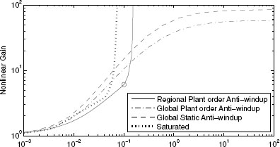
Figure 5.14 Nonlinear gains for Examples 4.3.3, 5.4.2, and 5.5.1 characterizing the system before and after static global (dotted), plant-order global (dashed-dotted), and plant-order regional (solid) anti-windup augmentation.

5.5.2 Regional full-authority reduced-order augmentation

Paralleling the full-authority construction introduced in Section 5.4.2 on page 122, reduced-order regional full-authority anti-windup can be achieved by suitably generalizing the static and plant-order constructions of Algorithms 3 and 8 on pages 99 and 143, respectively. In particular, in the regional full-authority case, when seeking for reduced-order anti-windup augmentation with a guaranteed performance level, the conditions at step 3 of Algorithm 3 and at step 2 of Algorithm 8 generalize to the following nonlinear conditions involving a nonlinear rank constraint and paralleling the full-authority conditions (5.16) seen in Section 5.4.2 on page 122:

Similar to the full-authority case on page 123, conditions (5.17) are not easily solvable because of the presence of the nonlinear rank constraint. It is, however, possible to solve a simplified problem whereby minimizing the trace of R — S results in generating a rank-deficient matrix, thereby reducing to a certain extent the size n_aw of the compensator. The approximate approach already adopted in the full-authority case can then be used also here to construct a triple (R*, S*, γ*) which serves as a starting point for reduced-order anti-windup design, where j* is close to a desired guaranteed performance level j_G.

A procedure is reported next which parallels (for the regional case) the global Procedure 2.

Procedure 4 (Computation of an (R, S, γ²) solution for reduced-order full-authority anti-windup with guaranteed performance)

Step a) A plant and a controller of the form (5.1), (5.2), and the matrices of the compact closed-loop representation constructed based on equations (5.5) and (5.8) are given. A maximum size s of allowable external inputs w₂>s over which the gain minimization has to be performed is given. Possibly, two matrices Sp and Rp are given, characterizing a desirable guaranteed reachable set contained in R_p = {x_p : x^T_p^{— 1}x_p} and a desirable stability region containing S_p = {x_p : xpS^{- 1}x_p} in the plant state directions, otherwise ignore the conditions involving S_p and R_p below. A small positive constant ε to robus-tify the closed-loop LMI condition and a value γ_G characterizing the desired guaranteed performance are also given. Note that the actual performance γ* achieved by the minimal-order (R, S, γ) solution will be, in general, larger than γ_G but often very close to it.

Step b) Find the optimal solution (R₁₁, S) ∈ ^np×np x ^{ncl x ncl nuXnp} to the following LMI eigenvalue problem:

Step c) Compute the SVD of the symmetric matrix R ₁₁ — S ₁₁ determined from the solution of the previous step. That is, compute F, Λsuch that FAF^T = R ₁₁ — S ₁₁, where A is a positive semidefinite diagonal matrix whose diagonal entries are nonincreasing (for example, use the MATLAB command.[U,Lamda, V] = svd(R11 - S11); F =(U+V)/2;). Set n_aw = n_p.

Step d) Call λ₁,…. λn_aw−1 entries on the diagonal of Λ and entries on the diagonal of Λ and define Λ := diag{γ₁…, γn_aw—1,0,…,0}. That is, Λis a diagonal matrix having its first n_aw −1 diagonal entries equal to the entries of Λ and the remaining entries equal to zero. Also define .

Step e) Given the matrix where Ŝ was determined at the previous step, verify the feasibility of the following LMI in the variable γ²:

If the LMI is feasible, then set (R*_1; S*, γ*) := (R_11; S, √ γ²), set n_aw = n_aw -1, and go to step d. If the LMI is not feasible, then go to step f.

Step f) Select the order of the anti-windup compensator as n_aw and the (R, S, γ) solution as (R*_1; S*, γ*).

In the worst case, Procedure 4 will give a solution (R, S, γ) characterizing an anti-windup compensation of order n_aw = n_p. However, several case studies confirmed that the reduced order obtained with this algorithm is very likely to be smaller than or equal to n_p. Clearly, its value depends on the level of guaranteed performance γ_G requested from the construction.

Once a triple (R*, S*, γ*) satisfying (5.19) with a small enough n_aw is determined from Procedure 4, the reduced-order anti-windup construction can be carried out following a simple generalization of the previous Algorithms 3 and 8, which is reported next.

Algorithm 9 (Dynamic reduced-order full-authority regional DLAW)

Step 1. Given a plant and a controller of the form (5.1), (5.2), construct the matrices of the compact closed-loop representation using (5.5) and (5.8). Select a small positive constant ε to robustify the order minimization procedure and a constant α > 1 characterizing the amount of performance to be traded in for order reduction. Select a constant v ∈ [0,1) used to enforce a strong well-posedness constraint (see Section 3.4.2 on page 60) and select the maximum size s of allowable external inputs w₂>s over which the gain minimization has to be performed.

Possibly select two matrices S_p and R_p characterizing a desirable guaranteed reachable set contained in R_p = {x_p : x_ppR _p-1x_p} and a desirable stability region containing S_p = {x_p : xpS^{- 1}x_p} in the plant state directions, otherwise ignore the conditions involving Sp and Rp below.

Step 2. Find the optimal solution (R ₁₁, S, γ, _np²)∈^npXnp× ⁿci^xnd _x ^nuXnp x R to the following LMI eigenvalue problem which is always feasible for small enough values of s:

The resulting performance level γ_np corresponds to the maximum performance achievable by plant-order anti-windup augmentation.

Step 3. Based on the matrices and parameters determined at step 1, select the desired guaranteed performance as γ_G = ay_n and determine the reduced compensator order n_aw and the triple Procedure 4.

Step 4. Based on the solution determined at the previous step, construct the symmetric matrix and the define Q₁₂ ∈ ^n_cl×n_aw solution to the following equation:

which is always solvable and admits infinitely many solutions because by construction, rank(RS^-1R - R) = rank((RS^-1R - R)(R^-1S)) = rank(R − S) = n_aw. A solution can be determined following Procedure 1 on page 113 with H = RS^—1R — R. Then define the following matrices:

Step 5. Based on the matrices determined at steps 1 and 4 define the following matrices (where the second row and column of zeros have size naw):

and construct the matrices Gu ∈^(naw+^nu)xm, H e∈^mx(naw+^ny+^nu), and Ψ∈^mXm, with m := n_cl + n_aw + n_u + n_w + n_z, as follows:

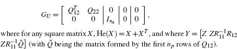
where for any square matrix X, He(X) = X + X^T, and where (with Q being the matrix formed by the first n_p rows of Q₁₂).

Step 6. Find the optimal solution (A_U, U, y²) of the LMI eigenvalue problem:

Step 7. Select the plant-order full-authority anti-windup compensator as:

with the selection

Example 5.5.2 (Electrical network) Consider the same example for which regional plant-order anti-windup has been designed in Example 5.5.1. The regional performance obtained there can be given up for an increased simplicity in the anti-windup architecture. Keeping the value s = 0.1 used in Example 5.5.1 and fixing a = 1.3 (so that y_G = 7.88 is obtained), Algorithm 9 provides the following first-order anti-windup compensator:

inducing a regional performance γ = 7. 35 (note that due to numerical reasons, this performance is slightly better than γG).

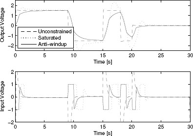
Figure 5.15 Plant output and input responses of various closed loops for Example 5.5.2.

Figure 5.15 represents a simulation showing how the reduced-order solution leads to a slightly slower response, as compared to the equivalent plant-order regional solution of Example 5.5.1. This slight deterioration of the closed-loop performance is also confirmed by the curves in Figure 5.16, where it is shown that the nonlinear gain curve of Example 5.5.1 (dashed) lies below the nonlinear gain curve of this example.

5.6 NOTES AND REFERENCES

Dynamic direct linear anti-windup designs are definitely more recent than the static anti-windup schemes discussed in the previous chapters. To the best of the authors’ knowledge, the first systematic LMI-based approach for dynamic anti-windup design appeared in in [MI18] (see also [MI19] for some case studies). Note, however, that alternative dynamic approaches to anti-windup had already appeared in [MR1, MR3, H1, H3] and other works. The full-authority work in [MI18] was later extended to the external case in [MI22]. It was also extended to the full-authority regional anti-windup case in [MI33]. Regional external anti-windup hasn't been published anywhere but is a straightforward extension of existing results. An alternative interesting approach is reported in [MI23], where an LMI-based procedure to minimize the URR gain instead of the L₂ gain reported here is given. This approach is not reported in this book to keep the discussion simple. The reduced-order anti-windup designs reported here are taken from [MI28]. Alternative reduced-order designs can be found in [MI25] as well as [MI31] and [MI34] and references therein.

Figure 5.16 Nonlinear gains for Examples 5.4.2, 5.5.1, and 5.5.1 characterizing the system before and after plant-order global (dashed-dotted), plant-order regional (dashed), and reduced-order regional (solid) anti-windup augmentation.

Discrete-time counterparts of the algorithms given here have been given in [MI30] (which can be seen as the discrete-time equivalent of the work in [MI18] and [MI33]).

The MIMO academic example no. 2 treated in Example 5.4.1 is taken from [MI11] even though it had appeared before in [FC7] (it was also revisited several times later, e.g., in [MI19]). The passive electrical circuit used in Examples 5.4.2, 5.4.6, 5.5.1, and 5.5.2 was introduced and used in [MI19] and later revisited in [MI22]. The SISO academic example no. 2 addressed in Examples 5.4.3, 5.4.5 and 5.4.8 was introduced in [MI16], where it was discussed that the quadratic construction of [MI11] was not always feasible (the system theoretic feasibility conditions appeared later in [MI18]). The F8 longitudinal dynamics example addressed in Examples 5.4.4, 5.4.7, and 5.4.9 first appeared in [SAT1] and was later revisited in a large number of papers (e.g., [MI18]).