
Chapter Four
Static Linear Anti-windup Augmentation
4.1 OVERVIEW
This chapter introduces the first constructive tools for anti-windup augmentation. According to the characterization of Section 2.3, the chapter addresses the simplest possible augmentation scheme that may induce on the closed loop the qualitative objectives discussed in Section 2.2, possibly in addition to some of the quantitative performance objectives of Section 2.4.
This chapter focuses on the “static linear anti-windup” augmentation architecture, wherein the difference between the input and the output of the saturation block drives a static linear system that injects modification signals into the unconstrained controller dynamics. The corresponding anti-windup filter structure is the simplest possible because it only consists of linear matrix gains of suitable dimensions.
Although the linear static anti-windup architecture is extremely simple, such is not the case for the algorithms that can be employed for the selection of the corresponding matrix gains. The class of algorithms considered in this chapter is based on linear matrix inequalities (which were introduced in Section 3.3) that, when appropriately solved, provide gain selections that correspond to optimal values of certain performance measures. The reason why only LMI-based algorithms are reported (despite a large literature on alternative rigorous or qualitative approaches) is that the resulting constructions have been proven to perform extremely well in many application cases and that once the reader gains confidence with the LMI mathematical tool and with a preferred LMI solver, the construction of optimal anti-windup gains becomes quite straightforward as the computational burden is carried out automatically by the software.
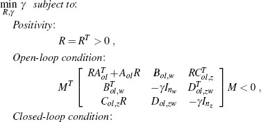
The performance measure optimized by all the algorithms discussed in this chapter is the input-output gain from the input signal w(·) to the performance output signal z(·) (recall that w(·) can contain both disturbances and references acting on the closed-loop system). Therefore, the algorithms reported next will aim at minimizing γ in the following inequality
either globally, namely, for arbitrarily large selections of w(·), or regionally, namely, for selections of w(·) below a certain bound.
Throughout the chapter, both full-authority and external anti-windup architectures will be addressed (according to the characterization in Section 2.3.6), although full-authority algorithms will be receiving more attention.
All the algorithms given in this chapter are based on the use of LMIs; thus, the corresponding stability and performance guarantees will rely upon the techniques outlined in Chapter 3.
4.2 KEY STATE-SPACE REPRESENTATIONS
Before introducing the anti-windup design algorithms, it is mandatory to introduce suitable state-space representations of the control systems under consideration. These representations will be both necessary to compute certain parameters needed in the anti-windup design algorithm and to allow use of the nonlinear gain calculation tools of Section 3.5.3 on page 66 on the compensated closed-loop systems determined from the algorithms.
The baseline saturated control system before linear anti-windup augmentation consists in the following linear systems: a plant with input saturation:
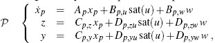
and a linear unconstrained controller:
For these two systems it will be useful to construct the matrices characterizing their interconnection in the absence of saturation. This interconnection can be represented in a compact way by stacking the two (plant + controller) states in a single state vector as ![]() . The corresponding state-space equations are given by the following compact closed-loop representation:
. The corresponding state-space equations are given by the following compact closed-loop representation:

where q = dz(u) encompasses the general effect of the nonlinearity on the otherwise linear control system.
Under the baseline assumption that the unconstrained interconnection between the plant (4.1) and the controller (4.2) is well-posed, the matrices appearing in (4.3) are uniquely determined by the values of the matrices in (4.1) and (4.2) as follows:

 (4.4b)
where the matrices Δu := (I − Dc,yDp,yu)−1 and Δy := (I − Dp,yuDc,y)−1 are well-defined as long as the unconstrained closed loop is well-posed.
The goal of static linear anti-windup augmentation is to design a suitable matrix gain Daw that is driven by the function q = dz(u) = u - sat(u) and that injects modifications on the controller equations (4.2), either based on a full-authority architecture or based on an external architecture. The resulting compensated closed loop is a simple extension of system (4.3) which incorporates the additional anti-windup signals, as follows:

where the matrices Bcl,v, Dcl,uv, and Dcl,zv depend on the architecture, full authority or external, of the compensation scheme under consideration. The values of these matrices are detailed separately for the two architectures in the following two sections.
4.2.1 Closed-loop representation with full-authority anti-windup
Full-authority static linear anti-windup augmentation corresponds to modifying the controller equations (4.2) as follows:
where the two signals v1 = Daw,1q and v2 = Daw,2q are injected in the state and output equation, respectively, with the goal of recovering closed-loop stability and performance. The matrix ![]() (namely, having nc + nu rows and nu columns) is the design parameter.
(namely, having nc + nu rows and nu columns) is the design parameter.
When adopting the full-authority architecture, the matrices Bcl,v, Dcl,uv, and Dcl,zv in (4.5) correspond to the following values:

After the anti-windup gains are designed by way of any of the full-authority algorithms reported in this chapter, the nonlinear performance of the resulting anti-windup compensation scheme can be evaluated relying on the LMI-based tools introduced in Section 3.5.3. To this end, it will be useful to use the following equations which show in explicit form the selection of the matrices in (3.54) that should be carried out to represent the static full-authority linear anti-windup architecture with that notation:

where ![]() Most of the examples provided in this chapter will in-corporate a nonlinear L2 gain analysis curve determined using transformation (4.8) and the tools of Section 3.5.3.
Most of the examples provided in this chapter will in-corporate a nonlinear L2 gain analysis curve determined using transformation (4.8) and the tools of Section 3.5.3.
4.2.2 Closed-loop representation with external anti-windup
Different from the full-authority case, in external static linear anti-windup augmentation, the modification signals denoted by v and enforced on the controller by the anti-windup gain are not allowed to access all the controller states but can only affect the external signals, namely, the controller input and output. The controller equations (4.2) then become:
where the two signals v1 = Daw,1q and v2=Daw,2q are injected, respectively at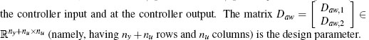
When adopting the external architecture, the matrices Bcl,v, Dcl,uv, and Dcl,zv in (4.5) correspond to the following values:

Similar to the static full-authority case, static linear external anti-windup schemes can also be analyzed by way of the nonlinear performance estimation tools of Section 3.5.3 on page 66. As in the full-authority case, the matrices in (3.54) should be selected using equation (4.8). However, for the external case, the matrices Bcl,v, Dcl,uv, and Dcl,zv must be selected as in (4.10)..
In the external anti-windup construction reported later in this chapter, certain LMIs will depend on the matrices corresponding to the state-space representation of the plant and of the unconstrained controller when they are disconnected. The corresponding dynamical system is referred to as compact open-loop representation and is described by the equations
where the input v1 resembles the first signal injected by the external anti-windup action and where the matrices correspond to the following selections:

4.3 ALGORITHMS PROVIDING GLOBAL GUARANTEES
The first family of algorithms considered in this chapter provides global stability and performance guarantees for the anti-windup closed loop. In particular, an optimized input-output gain will be guaranteed for the augmented closed loop. The desirable global guarantees given by these algorithms are obtained at the cost of a restricted applicability. Indeed, static direct linear global anti-windup will only apply to a strict subclass of the control systems with exponentially stable plants. More generic plants can be handled either by trading the global properties for regional ones, as shown later in this chapter, or by adopting dynamic compensators, as shown in the next chapter.
4.3.1 Global full-authority augmentation
Full-authority linear static anti-windup compensation synthesis amounts to selecting the matrices Daw,1 and Daw,2 of the static anti-windup compensator in Figure 4.1. An algorithm to construct such compensators is now offered.

Figure 4.1 Full-authority static anti-windup compensation scheme.
Note that the simplicity in the anti-windup structure (a simple linear gain) is a tradeoff for the lack of general applicability of the algorithm. In particular, the feasibility conditions at step 2 of the algorithm should be verified beforehand and if these don't admit a solution the reader should use alternative constructions (such as the regional static ones of Section 4.4 or the dynamic algorithms given in the next chapter).
Algorithm 1 (Static full-authority global DLAW)

Comments: Simple architecture, very commonly used but not necessarily feasible for any exponentially stable plant. Global input-output gain is optimized.
* Only those plants and unconstrained controllers satisfying step 2.
Step 1. Given a plant and a controller of the form (4.1), (4.2), construct the matrices of the compact closed-loop representation using (4.4) and (4.7). Select a constant v ∈ [0,1) used to enforce a strong well-posedness constraint (see Section 3.4.2 on page 60).
Step 2. Verify the applicability of this algorithm by checking the following feasibility conditions in the variable R:

If these conditions are not feasible, this algorithm is not applicable.
Step 3. Based on the matrices determined in step 1, find the optimal solution ![]() to the following LMI eigenvalue problem:
to the following LMI eigenvalue problem:

Step 4. Based on the matrices determined at step 1, construct the matrices ![]() with m := ncl + nu + nw + nz, as follows:
with m := ncl + nu + nw + nz, as follows:

where for any square matrix X, He(X) = X + XT.
Step 5. Find the optimal solution (ΛU, U, γ) of the LMI eigenvalue problem:

Step 6. Select the static full-authority anti-windup compensator as: v = Dawq with the selection Daw = ΛUU−1.
![]()
4.3.1.1 Interpretation of feasibility conditions*
The feasibility conditions at step 2 of Algorithm 1 characterize the class of control systems for which the static global anti-windup augmentation is applicable. A first fact that appears from the feasibility conditions is that both the plant and the unconstrained closed-loop system need to satisfy a Lyapunov equation; therefore, exponential stability of the plant is a necessary, and quite restrictive, assumption for Algorithm 1 to be applicable. Moreover, since the matrix R is the same in the LMI involving the plant and in the LMI involving the unconstrained closed loop, extra constraints are actually imposed by the feasibility conditions about a special type of compatibility between open-loop and closed-loop systems, as clarified next.
In the case where nc = 1, so that ncl = np, namely, the order of the unconstrained closed loop is the same as that of the plant, these conditions can be understood as requiring a single quadratic Lyapunov function, characterized by the matrix R–1, to decrease both along the trajectories of the closed-loop system and along the trajectories of the open-loop plant. In the more general case when nc > 0, the condition generalizes to what could be denoted as a “quasi-common” quadratic Lyapunov function between the unconstrained closed loop and the open-loop plant. To give further insight in the meaning of this feasibility condition, an example with nc = 0 and np = 2 is reported next so that the closed-loop trajectories can be visualized on the open-loop and closed-loop state space.
Example 4.3.1 Consider an exponentially stable linear plant P of the form (4.1) with matrices

and the following static unconstrained controller K:
with Dc,y = 1. The remaining plant and controller matrices are irrelevant to the feasibility discussion carried out in this example.
The unconstrained closed-loop matrix Acl constructed according to equation (4.4) is exponentially stable and corresponds to:

Figure 4.2 Phase portraits of the open-loop plant and unconstrained closed-loop systems in Example 4.3.1.
For this simple example, the feasibility conditions at step 2 of Algorithm 1 are not satisfied. Inspecting the phase portraits of the open loop and unconstrained closed loop, reported in Figure 4.2, reveals that it is not possible to define ellipses centered at the origin for which both the left and right trajectories are pointing inward. This is a graphical interpretation of the fact that there is no common quadratic Lyapunov function for the two systems, which is a necessary condition for Algorithm 1 to be applicable.![]()
4.3.1.2 Case studies
Even though Algorithm 1 has a restricted applicability, as illustrated in Example 4.3.1, whenever the plant is exponentially stable and the feasibility conditions at step 2 are satisfied, it constitutes a very simple and effective construction. Next, four examples are reported where, whenever feasible, this static DLAW design leads to extremely improved closed-loop responses (as compared to the saturated responses without anti-windup compensation).
The first example is an academic MIMO system. This example is useful to show how the direct linear anti-windup augmentation technique directly applies to systems with multiple inputs. For these systems, qualitative solutions may face severe problems related to the fact that the saturation nonlinearity changes the so-called “input directionality” thus causing undesired effects at the plant output. Since the approach of Algorithm 1 optimizes a performance measure involving the plant output, the resulting anti-windup compensation implicitly accounts for the input allocation and no extra effort is needed when dealing with MIMO plants. Indeed, as shown next, applying the algorithm in a straightforward manner leads to very desirable results.
Example 4.3.2 (MIMO academic example no. 2) Consider an exponentially stable plant that can be written in the form of (4.1) with matrices
and Bp,w = Dp,yw = 02x2 and suppose a controller has been designed of the form (4.2) with matrices

such that the unconstrained closed-loop system has a desirable decoupled unconstrained response (here the role of w is to be a vector reference). However, if a decentralized unit saturation limits the plant input then the plant has a very poor response. See the dotted line in Figure 4.3 for the plant output response to a reference changing from [0,0]T to [0.63, 0.79]T at time t = 0. The saturated closed-loop system peak magnitude output for y1 is -4.72 and for y2 is 4.75.

Figure 4.3 Plant output responses of various closed loops for Example 4.3.2. See legend in Table 4.1.
By choosing the performance output z = y − w, the remaining matrices of the plant are
For this example, the feasibility conditions at step 2 of Algorithm 1 hold, and with the selection v = 0.001, the algorithm yields the static full-authority anti-windup compensator gains

Figure 4.4 Plant input responses of various closed loops for Example 4.3.2. See legend in Table 4.1.

Table 4.1 Legend for the time histories in Figures 4.3 and 4.4.
which guarantee the performance level γ = 1.56. The step response of the resulting anti-windup closed-loop system is very much improved, as shown by the solid curves in Figures 4.3 and 4.4.
It is useful to point out that the algebraic loop resulting from the presence of a nonzero selection of Daw,1 in (4.13) becomes a key element to enforce a desirable output response. Indeed, this matrix is responsible for the input behavior of Figure 4.4, where the second input of the anti-windup response (solid curve in the lower plot) is forced to lie in the interior of the saturated region. This type of behavior would not be achievable by strictly proper compensators (namely, compensators with Daw,2 = 0) because the controller output exceeds the saturation limits on both inputs (this is evident from the saturated response [dotted curves in Figure 4.4], and only an implicit equation arising from an algebraic loop can instantaneously force the actual plant input within the interior of the linear region of the saturation.
The closed-loop performance of the static anti-windup compensator can be appreciated by inspecting the nonlinear gain of the augmented closed loop with anti-windup, which is represented in Figure 4.5 and compared to the gain before anti-windup compensation. These gains have been computed using the transformation (4.8) and the tools of Section 3.5.3. From this figure it is evident that the com

Figure 4.5 Nonlinear gains for Example 4.3.2 characterizing the system before and after anti-windup augmentation.
pensation leads to a dramatic gain improvement (note that the scale in the figure is logarithmic). It is also instructive to observe that the anti-windup compensation was designed to optimize the global L2 gain, namely, the gain for very large values of the input size, which led to the optimal value γ = 1.561, corresponding to the far right of the solid curve in Figure 4.5.![]()
The next example represents a model of an electrical network where static anti-windup is feasible and performs well. For this example, it will be shown in the next chapter that dynamic anti-windup can lead to improved performance.
Example 4.3.3 (Electrical network) Consider the passive electrical circuit in

Figure 4.6 The passive electrical circuit of Example 4.3.3.
Figure 4.6, where the control input is the voltage Vi and the measurement output coincides and corresponds to the voltage Vo. The resistors and capacitor values are selected as R1 = 313Ω, R2 = 20Ω, R3 = 315 Ω, R4 = 17Ω, R5 = 10Ω, and C1 = C2 = C3 = 0.01 F. The gain k is selected so that the transfer function from Vi to Vo is monic. This function can be easily computed as
Based on the above transfer function, a state-space representation for this circuit
can be easily derived (e.g., using the function ssdat a of MATLAB) as

and since there's no disturbance in the problem setting, Bp,w = 03 × 1 and Dp,yw = 0. The following approximate PID controller can be used to robustly stabilize the unconstrained closed loop and to induce a desirable step response. The controller induces an infinite gain margin and a phase margin of 89.5 degrees:

where w = r corresponds to the reference input for the desired value of the output voltage Vo.
When input saturation is present at the input voltage Vi, the saturated closed loop experiences windup and is in need of anti-windup compensation. In particular, the control input is saturated here between the maximum and minimum voltages ±1 V and a global static full-authority anti-windup compensator is designed following Algorithm 1 selecting v = 0.1. For the algorithm to optimize the gain from the reference input r = w and the output tracking error e = r − y, the performance output matrices of the plant (4.1) are selected as Cp,z = Cp,y, Dp,zu = Dp,yu, and Dp,zw = Dp,yw − 1. The feasibility conditions at step 2 of Algorithm 1 are satisfied for this example; therefore, the algorithm provides a solution to the windup problem corresponding to the selection
which guarantees the global performance level γ = 85.22.
Figure 4.7 reports the input and output of the plant when the unconstrained, saturated and anti-windup closed loops are driven by a reference signal of doublet type, switching between +1.5V and −1.5V at increasingly narrow time intervals and finally going back to zero. The simulation results show unacceptable overshoots characterizing the saturated responses and demonstrate the effectiveness of anti-windup augmentation in mitigating this undesired effect. Nevertheless, the anti-windup response is quite slow and it will be shown in the following sections that when using dynamic (see Example 5.4.2 on page 118) or regional static (see Example 4.4.2 on page 104) anti-windup, improvements will be achieved on the speed of convergence of the anti-windup response.
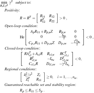
Figure 4.8 reports the nonlinear gains characterizing the closed loop before and after anti-windup. These gains have been computed using the transformation (4.8) and the tools of Section 3.5.3. Inspecting the nonlinear gains it appears that the saturated closed loop before anti-windup admits a regional gain only up to the value s ≈ 0.075. Above that value, either the saturated closed loop loses external stability or the quadratic tools adopted to establish this gain curve are too conservative.
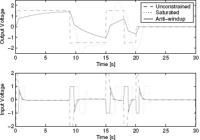
Figure 4.7 Plant output and input responses of various closed loops for Example 4.3.3.

Figure 4.8 Nonlinear gains for Example 4.3.3 characterizing the system before and after anti-windup augmentation.
Conversely, the nonlinear gain computed after anti-windup compensation shows external stability for any reference input size and confirms the global performance level γ = 85.22 provided by the optimal anti-windup design algorithm and corresponding to the far right value of the solid curve in Figure 4.8.![]()
In the next example static compensation is not feasible. The simplicity of the example, which involves a SISO plant with two internal states, indicates that there are situations where even elementary anti-windup problems require dynamic compensation for global results based on quadratic Lyapunov functions. The example will be revisited in the following chapter where dynamic DLAW designs will be introduced.
Example 4.3.4 (SISO academic example no. 2) Consider the following SISO plant without any disturbance input:

Consider the following one-dimensional controller selection for the SISO plant introduced above:
When the control input is saturated between ±0.5, the saturated closed loop exhibits very large oscillations with extremely long settling time. It is therefore of interest to design anti-windup augmentation for this closed loop. Unfortunately, for this example the feasibility conditions at step 2 of Algorithm 1 do not admit a solution. Therefore the algorithm cannot be applied and it is necessary to adopt the alternative tools provided later in the book, namely, either the regional static anti-windup tools illustrated for this problem setting in Example 4.4.2 later in this chapter or the dynamic anti-windup tools illustrated in Example 5.4.3 and 5.4.5 in the next chapter.![]()
![]()
The example introduced in Section 1.2.3 of the introductory chapter on page 8 is revisited next. For this example, static full-authority anti-windup design is feasible and is effective in reducing the windup effects.
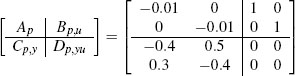
Example 4.3.5 (F8 longitudinal dynamics) The linearized longitudinal dynamics of an F8 aircraft can be represented by the following selections for the linear plant (4.1)

where the two inputs correspond to the elevator angle and to the flaperon angle, respectively, and the two outputs correspond to the pitch angle and the flight path angle. No disturbances are taken into account for this example; therefore, the external signal w consists only in two references specifying the desired values at the two plant outputs. As a consequence, the plant matrices related to the input w are zero: Bp,w = 04x2, Dp,yw = 02x2. The performance output z is selected in such a way that two suitable combinations of the plant state are penalized, thereby leading to desirable responses of the compensated closed loop. In particular, the plant matrices related to z are selected as:
The controller for the F8 dynamics is selected based on an LQG/LTR methodology applied to an augmented plant having two extra integrators to guarantee asymp totic tracking of constant references. The overall controller state-space representation corresponds to:

where

and the controller parameters G and H are selected as


Figure 4.9 Plant output responses of various closed loops for Example 4.3.5.
The unconstrained interconnection of this controller with the F8 longitudinal dynamics model behaves very desirably and guarantees fast and smooth responses to step references for both the regulated outputs. However, if the control inputs are both saturated between ±25 degrees, namely, ![]() the saturated response exhibits unacceptable oscillations. This phenomenon is illustrated in Figures 4.9 and 4.10 representing the plant output and input responses, where the unconstrained behavior corresponds to the dashed curves and the saturated one corresponds to the dotted curves.
the saturated response exhibits unacceptable oscillations. This phenomenon is illustrated in Figures 4.9 and 4.10 representing the plant output and input responses, where the unconstrained behavior corresponds to the dashed curves and the saturated one corresponds to the dotted curves.
Algorithm 1 can be used to design a static full-authority anti-windup compensator for this example because the feasibility conditions in step 2 of the algorithm
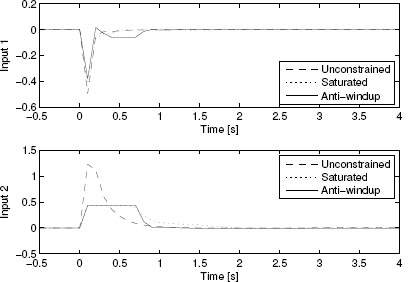
Figure 4.10 Plant input responses of various closed loops for Example 4.3.5.
are satisfied. Selecting v = 0.005, the following anti-windup gains are obtained:

which induce a global performance level γ = 26.44. The corresponding anti-windup response corresponds to the solid curves in Figures 4.9 and 4.10, that show a significant mitigation of the windup phenomenon, although they present a slowly decaying transient that might be nonacceptable for implementation. This transient will be removed when relying on the dynamic anti-windup schemes of the next chapter (see Example 5.4.4 on page 121 and Example 5.4.7 on page 133).
The nonlinear gains of the closed loop before and after anti-windup augmentation are represented in Figure 4.11. It is worthwhile pointing out that these gains were computed after increasing the default accuracy of the MATLAB LMI control toolbox solver. From the gains it appears that static anti-windup significantly improves the external stability properties of the closed loop.![]()
4.3.2 Global external augmentation
As compared to the full-authority case, external linear static anti-windup compensation corresponds to allowing the linear anti-windup gain to only affect the unconstrained controller external signals, namely, its input and output. The corresponding block diagram is shown in Figure 4.12 where Daw,1 and Daw,2 are the design parameters.
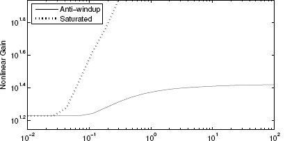
Figure 4.11 Nonlinear gains for Example 4.3.5 characterizing the system before and after anti-windup augmentation.

Figure 4.12 External static anti-windup compensation scheme.
Since external anti-windup augmentation is a special case of full-authority augmentation, the degrees of freedom available to external anti-windup for performance and stability purposes are less than those available in the full-authority case. As a consequence, the feasibility conditions of the following algorithm will be more stringent than those of full-authority anti-windup. The payoff for this is that whenever feasible, external anti-windup will lead to compensation gains of smaller dimension, therefore of easier implementation.
Algorithm 2 (Static external global DLAW)

Comments: Useful when some internal states of the controller are inaccessible. Otherwise not more effective than Algorithm 1. Global input-output gain is optimized.
* Only those plants and unconstrained controllers satisfying step 2.
Step 1. Given a plant and a controller of the form (4.1), (4.2), construct the matrices of the compact closed-loop representation using (4.4) and (4.10) and the matrices of the compact open-loop representation using (4.12). Select a constant v ∈ [0,1) used to enforce a strong well-posedness constraint (see Section 3.4.2, page 60). Moreover, based on the matrix Bo1,v in equation (4.12), generate any matrix Bol,V⊥ that spans the null space of its transpose, such that BTol,v⊥Bol,v = 0 and rank(Bol,v⊥) + rank(Bol,V) = nc + np. (Note that in general there can be infinite selections of Bol,v⊥ As an example, using MATLAB, an orthonormal selection of Bol,v⊥ is easily computed using Bolperp = null(Bolv).)
Step 2. Verify the applicability of this algorithm by checking the following feasibility conditions in the variable R:

If these conditions are not feasible, this algorithm is not applicable.
Step 3. Define  . Based on the matrices determined at step 1, find the optimal solution
 ![]() of the following eigenvalue problem:
of the following eigenvalue problem:

Step 4. Based on the matrices determined at step 1, construct the matrices ![]() as follows:
as follows:

where for any square matrix X, He(X) = X + XT.
Step 5. Find the optimal solution (ΛU, U, γ) of the LMI eigenvalue problem:

Step 6. Select the static external anti-windup compensator as: v = Dawq with the selection Daw = ΛUU−1.
![]()
4.3.2.1 Interpretation of feasibility conditions*
The feasibility conditions for static external anti-windup augmentation with global guarantees correspond to the LMIs listed at step 2 of Algorithm 2. It is instructive to compare these conditions to the corresponding ones for the full-authority case, reported at step 2 of Algorithm 1 on page 82, the latter ones having been commented on on page 83.
First observe that when Bc,u is a square invertible matrix, so that all the controller state equations can be independently modified from the controller input, external anti-windup reduces to being full-authority anti-windup. In that case, since the lower block of Bol,v in equation (4.12) is full rank, it is straightforward to verify that ![]() and that by (4.12), the external feasibility conditions of Algorithm 2 reduce to the full-authority feasibility conditions of Algorithm 1. According to the interpretation already given on page 83, these conditions require that there be a “quasi-common” quadratic Lyapunov function for the open-loop plant and the closed-loop system.
and that by (4.12), the external feasibility conditions of Algorithm 2 reduce to the full-authority feasibility conditions of Algorithm 1. According to the interpretation already given on page 83, these conditions require that there be a “quasi-common” quadratic Lyapunov function for the open-loop plant and the closed-loop system.
In the more general case where the matrix Bc,u is not square, the external feasibility conditions are evidently more stringent than the full-authority feasibility conditions, so that whenever the external static anti-windup construction is feasible, the full-authority one is feasible too. Conversely, whenever the full-authority scheme is not feasible, the external one is not feasible either. This fact becomes quite intuitive when recognizing that external anti-windup has fewer degrees of freedom than full-authority anti-windup because it is unable, in general, to independently modify each one of the internal controller state equations: it can only operate through the input matrix Bc,y. Once again, exponential stability of the open-loop plant becomes then a necessary assumption for the applicability of Algorithm 2 and even more strict requirements are imposed by the external feasibility conditions, as clarified next.
A deeper understanding of the external feasibility conditions arises from applying the following simple fact that can be proven by applying Finsler's lemma (see page 54):
Given a symmetric matrix Ξ and a matrix B having the same number of rows, construct any matrix B⊥ orthogonal to B such that BTB⊥ = 0. Then the following statements are equivalent:
1. B⊥ ΞB⊥ < 0.
2. There exists a matrix K of suitable dimensions such that Ξ + He(BK) < 0.
In light of this fact and based on equations (4.12), it is possible to replace the open-loop condition at step 2 of Algorithm 2 by the following equivalent condition in the variables ![]() and R:
and R:
which, based on the structure of Aol and Bol,v in (4.12) and performing the change of variable ![]() , becomes:
, becomes:
The last condition corresponds to requiring that there exist a static state feedback law Kxol for the compact open-loop representation which, injected at the controller input, guarantees quadratic stability with the Lyapunov function Vext := xTolR−1xol. It is standard notation in systems theory to call the function Vext a “control Lyapunov function” for the compact open-loop representation.
In light of this definition, of the conditions at step 2 of Algorithm 2, and of the interpretation above, the feasibility conditions for static external anti-windup augmentation can be stated as the existence of a single quadratic Lyapunov function Vext which is both a Lyapunov function for the compact unconstrained closed-loop system and a control Lyapunov function for the compact open-loop representation.
4.3.2.2 Case studies
The first two examples considered here show that in some cases the static external DLAW scheme performs as well as the full-authority one of Algorithm 1. The advantage in using external designs for those cases is that the anti-windup gains have smaller dimensions; therefore the on-line implementation is less computationally intensive.
Example 4.3.6 (MIMO academic example no. 2) Consider the problem described in Example 4.3.2 on page 85. For this particular example, the whole controller state is directly reachable from the controller input, so that external anti-windup is in principle equivalent to full-authority anti-windup. This equivalence is confirmed by the numerical optimization of Algorithm 2 which, when applied to this example, gives an external solution completely equivalent to the full-authority one of Example 4.3.2. In particular, picking v = 0.001, the gains given by Algorithm 2 are
and the guaranteed global performance is γ = 1.56. The nonlinear gain curve of the compensated system perfectly coincides with that of Figure 4.5 on page 87, characterizing the full-authority solution. Clearly, for this example there's no difference in picking full-authority or external DLAW compensation.![]()
Example 4.3.7 (Electrical network) Consider the same problem addressed in Example 4.3.3 on page 87. Similar to the previous example, external anti-windup leads to almost no performance deterioration. However, in this case there is an advantage in using the external architecture as the dimension of the anti-windup gains is in this case smaller. Selecting v = 0.1, the optimal gains resulting from Algorithm 2 are the following ones:
which guarantee the global performance is γ = 86.32, slightly deteriorated from the full-authority case of Example 4.3.3. Nevertheless, both the simulations and the nonlinear gain curve using the two schemes are indistinguishable from each other. This makes the external solution more desirable due to its simpler architecture.![]()
Even though the last two examples suggest that the external anti-windup scheme might be as effective as the full-authority one, this is not the case in general. There are cases, indeed, where static full-authority anti-windup compensation will be feasible and the external one won't be. This is shown in the next example.
Example 4.3.8 (F8 longitudinal dynamics) Consider the example introduced in Section 1.2.3 and revisited in Example 4.3.5, where static full-authority anti-windup has been designed for it.
For this example, the feasibility conditions at step 2 of Algorithm 2 are not satisfied; therefore global external linear compensators for this problem can only be determined among the family of dynamic compensators whose construction is the subject of the next chapter. Indeed, in the next chapter this example will be revisited and both a plant-order and a reduced-order dynamic linear anti-windup compensator will be designed for it.![]()
4.4 ALGORITHMS PROVIDING REGIONAL GUARANTEES
This section focuses on static linear anti-windup design algorithms that may overcome certain limitations of the algorithms provided in the previous section. These limitations arise from the fact that the previous algorithms only provide solutions enforcing global stability and performance properties. While these properties are very desirable, the price to be paid for them is often too high, sometimes because the resulting performance is not satisfactory enough for the problem under consideration, at other times because the algorithms may in some cases not be applicable at all because the feasibility conditions are often not satisfied.
The algorithms addressed in this section will provide a good alternative when it is known that the system will operate in a subset of the whole space and global guarantees are not necessary for the problem under consideration. It will be shown that giving up on the global guarantees will lead to weaker feasibility conditions and will remove the requirement that the open-loop plant be exponentially stable, which is overkill in many cases of interest. On the other hand, since only regional closed-loop guarantees are provided by these algorithms, large enough signals could drive the anti-windup closed-loop system unstable, or poor performance could be experienced if signals become too large. Nevertheless, in many practical cases, the tools provided here are the only ones suitable for anti-windup augmentation and their use may lead to radical stability and performance improvements in the operating conditions of the system under consideration.
From the nonlinear performance viewpoint (see Section 2.4.4), the algorithms provided next aim at finding anti-windup gains that optimize the value of the nonlinear gain curve at a certain horizontal position (namely, for a certain bound on ||w||2). Although no stability or performance guarantees for larger values of ||w||2 arise from the construction algorithms, it is often the case that an analysis carried out after the anti-windup design will reveal that the system is well behaved in very large regions. This type of afterdesign analysis will be carried out for the examples considered in this section.
Only full-authority regional algorithms will be presented here, although external ones can also be formulated slightly extending the results currently available in the literature. External algorithms will possibly be included in a subsequent edition of this book.
4.4.1 Regional full-authority augmentation
Regional static full-authority anti-windup augmentation shares the same architecture as the global counterpart addressed in Section 4.3.1 and amounts to selecting two matrices, Daw,1 and Daw,2, interconnected to the control system as represented in Figure 4.1.
An important difference between the regional and the global approaches is that when only regional properties are guaranteed, it becomes important to characterize the size of the stability region and of the reachable region from bounded inputs. The former region characterizes the set of initial states that lead to exponentially converging responses, while the second region indicates how large the state can grow when the closed loop is excited by an external input w with bounded L2 norm. In the following algorithm, estimates of both these regions will be automatically given, possibly allowing one to enforce a desired and prescribed guaranteed size in the direction of the plant states.
An interesting peculiarity of the algorithm given next is its dependence on the saturation levels ![]() i > 0, i = 1,…, nu, which may all be different from each other. The algorithm leads to solutions with guaranteed stability and performance also for time-varying saturation limits, as long as the vector
i > 0, i = 1,…, nu, which may all be different from each other. The algorithm leads to solutions with guaranteed stability and performance also for time-varying saturation limits, as long as the vector ![]() = [
= [![]() 1;…,
1;…, ![]() nu]T is a lower bound for the saturation values at all times. As a consequence, the algorithm is also applicable to nonsymmetric saturations as long as for each input channel the value ui, i =∈ {1,…, nu} is selected as the most stringent saturation limit for that channel. In this case, the stability and performance estimates provided by the algorithm increase in conservativeness.
nu]T is a lower bound for the saturation values at all times. As a consequence, the algorithm is also applicable to nonsymmetric saturations as long as for each input channel the value ui, i =∈ {1,…, nu} is selected as the most stringent saturation limit for that channel. In this case, the stability and performance estimates provided by the algorithm increase in conservativeness.
Algorithm 3 (Static full-authority regional DLAW)

Comments: Extends the applicability of Algorithm 1 to a larger class of systems by requiring only regional properties. However, feasibility conditions still need to hold. Regional input-output gain is optimized.
Step 1. Given a plant and a controller of the form (4.1), (4.2) and input saturation values ![]() , i = 1,…, nu, construct the matrices of the compact closed-loop representation using (4.4) and (4.7). Select a constant v ∈ [0,1) used to enforce a strong well-posedness constraint (see Section 3.4.2 on page 60) and select the maximum size s of allowable external inputs ||w||2 < s over which the gain minimization has to be performed.
, i = 1,…, nu, construct the matrices of the compact closed-loop representation using (4.4) and (4.7). Select a constant v ∈ [0,1) used to enforce a strong well-posedness constraint (see Section 3.4.2 on page 60) and select the maximum size s of allowable external inputs ||w||2 < s over which the gain minimization has to be performed.
Possibly select two matrices Sp and Rp characterizing a desirable guaranteed reachable set contained in ![]() and a desirable stability region containing
and a desirable stability region containing ![]() in the plant state directions, otherwise ignore the conditions involving Sp and Rp below.
in the plant state directions, otherwise ignore the conditions involving Sp and Rp below.
Step 2. Verify the applicability of this algorithm by checking the following feasibility conditions in the variables R and Z:
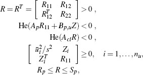
where Zi denotes the ith row of the matrix Z. If these conditions are not feasible, either this algorithm is not applicable or the parameters at step 1 should be selected differently.
Step 3. Based on the matrices determined at step 1, find the optimal solution ![]() to the following LMI eigenvalue problem:
to the following LMI eigenvalue problem:
Step 4. Based on the matrices determined at step 1, construct the matrices ![]() as follows:
as follows:

Step 5. Find the optimal solution (ΛU, U, γ) of the LMI eigenvalue problem:


Step 6. Select the static full-authority anti-windup compensator as: v = Dawq, with the selection Daw = ΛUU−1.
![]()
4.4.1.1 Interpretation of feasibility conditions*
It is instructive to compare the feasibility conditions at step 2 of Algorithm 3 to the corresponding feasibility conditions for the global static anti-windup design of Algorithm 1 on page 82.
A first important difference lies in the fact that the open-loop condition has now a new degree of freedom consisting in the variable Z, which allows one to overcome the severe applicability limit of the global algorithms: exponential stability of the plant. The role played by Z is quite interesting when understood in conjunction with the nu conditions involving each of the saturation limits ui, i = 1,…, nu. For each i, these conditions can be rewritten by using the Schur complement as ![]() so that two facts become evident:
so that two facts become evident:
1. the more stringent the saturation limits ![]() 2i are, the smaller the variable Z will be constrained to be,
2i are, the smaller the variable Z will be constrained to be,
2. the larger the size s of allowable external signals is, the smaller the variable Z will be constrained to be.
Imposing that Z be small affects its capability to satisfy the open-loop feasibility constraint, so that at the limit when s goes to infinity (global external stability), Z will be zero and the global limitations of Algorithm 1 will be recovered. Nevertheless, choosing a reasonable value for s and assuming that the saturation limits are compatible with its selection, Z will have enough degrees of freedom to allow the open-loop feasibility constraint to be satisfied.1
Similar to the external anti-windup conditions commented on on page 4.3.2.1, the open-loop condition in step 2 of Algorithm 3 can be interpreted in terms of control Lyapunov functions; as a matter of fact, with the variable change Z →Kp=ZR-111 the open-loop feasibility condition becomes:
which, combined with the closed-loop condition, has a nice system theoretic interpretation: if nc = 0 so that ncl = np, the function V = xTR−1x is both a quadratic Lyapunov function for the unconstrained closed loop and a quadratic control Lya-punov function for the open-loop plant from the control input. The coupling condition could in some examples impose applicability limitations that are too severe. Those limitations can be overcome by applying the dynamic regional anti-windup compensation algorithms of the next chapter.
An important aspect of the feasibility conditions for Algorithm 3 is that the regional properties of the algorithm can be quantified by imposing a prescribed guaranteed size for the reachable set from bounded inputs and for the region of attraction, namely, the region of initial conditions that lead to exponentially converging responses. This is done by way of the matrices Rp and Sp, respectively, as noted in step 1 of the algorithm. It should be emphasized, however, that larger values of Rp and smaller values of Sp make the feasibility constraints less likely to be fulfilled; therefore the selection of Rp and Sp should always be carried out within a certain reasonable range.
4.4.1.3 Case studies
The next example is useful to illustrate a situation where the windup effect is not caused by the reference input but by the disturbance input. In many cases problems induced by the reference input can be avoided by adding a suitable prefiltering action. However, when windup is triggered by disturbances, this is hardly possible and anti-windup is even more important to adopt.
Example 4.4.1 (A disturbance rejection problem) Consider the disturbance rejection problem corresponding to the block diagram representation in Figure 4.13, where the plant characterized by the following transfer function:
is subject to an input disturbance du(t) and its measurement y(t) is affected by the output noise dy(t). Suppose that the plant control input u(t) is subject to a saturation level of ±15 and that both the input and output disturbance are band-limited white noises. The input disturbance du(t) is a low-frequency noise that needs to be rejected by the active disturbance rejection system: it has noise power equal to 1 and a sample time of 0.2 seconds. The output disturbance dy(t) instead is a high-frequency noise affecting the measurement signal: it has noise power equal to 5.10−8 and a sample time of 5.10−3 seconds.

Figure 4.13 The disturbance rejection problem of Example 4.4.1.
For this example, the following controller is designed using a loop shaping technique with the goal of attenuating the low-frequency input disturbance by cranking up the low-frequency gain while preserving a certain level of stability margin:
This controller performs well during normal operation and induces extreme disturbance attenuation at the plant output corresponding to −60 dB attenuation for frequencies below ωl = 0.5 rad/s. Moreover, the loop gain at high frequencies is small enough that the control system is not too sensitive to measurement noise above ωh = 100 rad/s.

Figure 4.14 Plant output and input responses of various closed loops for Example 4.4.1.
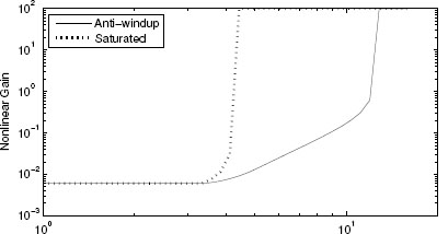
Figure 4.15 Nonlinear gains for Example 4.4.1 characterizing the system before and after anti-windup augmentation.
Assume now that at time t = 1 a pulse disturbance of amplitude 100 and length 0.1 seconds is added to the input disturbance du(t). Then the closed loop becomes unstable, as shown in Figure 1.28 on page 21 of the introductory chapter. The solution to this problem is easily obtained by transforming the transfer functions above into equivalent state-space representations and running Algorithm 3. Note that since the plant is not exponentially stable (due to the presence of a pole at the origin), all the global anti-windup algorithms provided in this chapter are infeasible. In Algorithm 3, the parameters v = 0.1 and s = 5 are selected. The algorithm provides the following static anti-windup compensator:

inducing the regional L2 performance γ = 0.0132. Figure 4.14 represents the simulation results with anti-windup compensation. It is evident that anti-windup is able to recover stability and fast disturbance rejection recovery. The saturated closed loop instead experiences the onset of persistent oscillations. Figure 4.15 represents the nonlinear L2 gains before and after anti-windup compensation. Note that unlike in the previous examples, which guaranteed global properties, regional anti-windup here only increases the guaranteed stability region. This is a necessary fact because no anti-windup action can induce global finite L2 gain for this example where the plant is not exponentially stable. ![]()
Example 4.4.2 (SISO academic example no. 2) In Example 4.3.4 on page 89 earlier in this chapter, a problem setting has been discussed where global static full-authority anti-windup design is not feasible, and therefore a static solution to the underlying anti-windup problem could not be given. For the same problem statement, namely, a SISO plant with an integrating one-dimensional controller, a regional anti-windup solution is given here. The saturation value is given by ![]() = 0.5. The plant and controller matrices are reported next for convenience:
= 0.5. The plant and controller matrices are reported next for convenience:

Algorithm 3 can be used for this example. Selecting v = 0.1 and s = 1 at step 1 of the algorithm leads to the following solution:
Daw,1 = -1.07, Daw,2 = 0.6,
which guarantees the regional performance level γ = 2.712 for any input having size ||w||2 ≤ 1. Figure 4.16 represents the plant input and plant output responses of the various closed loops when the reference input is selected as a step having amplitude 2. From the plot it is evident that regional anti-windup succeeds in mitigating the windup effects of the saturated closed loop.
Figure 4.17 represents the nonlinear gains characterizing this example before and after anti-windup augmentation. The system after anti-windup compensation is clearly more performing, although both the closed loops with and without anti-windup admit a quadratic linear gain only up to a certain value of the input size (roughly, up to s = 0.35 for the saturated closed loop and up to s = 2.04 for the anti-windup case). Note that for s = 1 the nonlinear gain curve passes through the value γ = 2.712, which has been established by the optimal design algorithm.![]()

Figure 4.16 Plant output and input responses of various closed loops for Example 4.4.2.

Figure 4.17 Nonlinear gains for Example 4.4.2 characterizing the system before and after anti-windup augmentation.
Example 4.4.3 (Electrical network) Consider the passive electrical circuit introduced in Example 4.3.3 and the resulting windup-prone control system. For that system both global full-authority and external anti-windup gains could be designed, but the resulting performance was quite sluggish (see the simulations in Figure 4.7 on page 89).
That windup problem can be tackled using a regional approach by way of Algorithm 3. In particular, selecting v = 0.1 and s = 0.01 in step 1 of the algorithm leads to the following solution:
which guarantees the regional performance level γ = 1.643 for any input having size ||w||2 ≤0.01. Figure 4.18 represents the plant input and plant output responses of the various closed loops when using the same reference input that was used in Figure 4.7 on page 89. Note that the regional design is able to induce an improved response for this specific trajectory selection. However, due to the regional properties of the approach, there are no guarantees on the closed-loop behavior for larger references.

Figure 4.18 Plant output and input responses of various closed loops for Example 4.4.3.

Figure 4.19 Nonlinear gains for Example 4.4.3 compared to the nonlinear gain from the global approach of Example 4.3.3.
The nonlinear gain characterization reported in Figure 4.19 shows that in the small signals range the regional approach (dashed curve) is more desirable than the global one (solid curve). It remains unclear why the nonlinear gain characterizing the closed loop before anti-windup (dotted curve) is so close to the regional one, despite the significant differences in the responses of Figure 4.18. This might be due to the limitations in the L2 gain characterization of performance or due to the conservativeness arising from the use of quadratic Lyapunov functions for the estimation of the nonlinear gains.![]()
Example 4.4.4 (MIMO academic example no. 2) Consider the problem statement considered first in Example 4.3.2 on page 85. One might wish that regional anti-windup would lead to improved nonlinear performance, at least for small values of ||w||2. However, when applying Algorithm 3 with s = 1 and v = 0.01, the following anti-windup gains are obtained:
which lead to a guaranteed regional performance level γ = 1.1. However, the simulations resulting from this regional gain selection are equivalent to the global ones reported in Example 4.3.2 and, most interestingly, the nonlinear L2 gain appears worse than that obtained for the global case. In particular, in Figure 4.20 the nonlinear gain obtained with regional anti-windup is compared to the one corresponding to global anti-windup (which comes from Figure 4.5 on page 87). In Figure 4.20, the small circle denotes the optimized regional gain, which in this case is just as good as the value of the nonlinear gain characterizing global anti-windup. However, since only regional guarantees are provided by Algorithm 3, the dashed curve for s » 1 is significantly deteriorated. For this specific example, global anti-windup appears to be more desirable than regional anti-windup.![]()
Figure 4.20 Nonlinear gains for Example 4.4.4 compared to the nonlinear gain obtained for the global design of Example 4.3.2.
4.5 NOTES AND REFERENCES
Static anti-windup was for many years the predominant type of anti-windup employed. An important survey of how several anti-windup schemes could have been written within the static anti-windup framework is [SUR4]. Perhaps the first paper casting anti-windup as an LMI optimization is [MI2, MI1]. In [MI11], Mulder, Kothare, and Morari cast global, static full-authority anti-windup synthesis with algebraic loops as an LMI. In [MI18] (see also [MI19] for some case studies), Grimm et al. provided the system theoretic interpretation of the feasibility conditions, as reported at the end of Section 4.3.1. The algorithms reported here for regional performance using static anti-windup first appeared in [MI27] (which can be interpreted as the regional counterpart of [MI11]). Then, in [MI33] (which can be interpreted as the regional counterpart of [MI18]), the system theoretic interpretations of regional static anti-windup were given. The external anti-windup schemes here presented are taken from [MI22] which extends the full-authority results of [MI18] to the external case also giving system theoretic interpretation. Regional external anti-windup hasn't been published anywhere but is a straightforward extension of existing results. An alternative interesting approach is reported in [MI23], where an LMI-based procedure to minimize the URR gain instead of the L2 gain reported here is given. This approach is not reported in this book to keep the discussion simple.
All the algorithms given here rely on the application of the so-called “elimination lemma” (see [G17]) to the anti-windup problem. This type of approach was first proposed in [G5] and [G6] to address the H∞ controller synthesis problem. The explicit formulas given in [G8] can also be used to bypass the last large LMI to be solved in the algorithms given in this chapter, which often causes numerical problems with large state-space dimensions. As an example, see [MI26], where those explicit formulas have been used for anti-windup design.
Discrete-time counterparts of the algorithms given here have been given in [MI24] (which can be seen as the discrete-time equivalent of the work in [MI11]) and in [MI30] (which can be seen as the discrete-time equivalent of the work in [MI18] and [MI33]).
Extensions of the direct linear LMI-based static anti-windup approaches to the case of systems with magnitude and rate saturations have been given in [MI32, MI29]. Those algorithms are not covered here, to keep the discussion simple.
The infeasible example for static anti-windup given in Example 4.3.1 was proposed in [MI18] where it was used to illustrate the feasibility conditions for static anti-windup. The MIMO academic example no. 2 treated in Examples 4.3.2, 4.3.6, and 4.4.4 is taken from [MI11] even though it had appeared before in [FC7] (it was also revisited several times later, e.g., in [MI19]). The passive electrical circuit described in Examples 4.3.3, 4.3.7, and 4.4.3 was introduced and used in [MI19] and later revisited in [MI22]. The SISO academic example no. 2 described and addressed in Examples 4.3.4 and 4.4.2 was introduced in [MI16], where it was noted that the quadratic construction of [MI11] was not always feasible (the system theoretic feasibility conditions appeared later in [MI18]). The F8 longitudinal dynamics example described in Examples 4.3.5 and 4.3.8 first appeared in [SAT1] and was later revisited in a large number of papers (e.g, [MI18]).
1 Requiring that the saturation limits be compatible with the size of the required stability region amounts to requiring that the actuators have a reasonable dimension for the control application under consideration.