
Chapter Three
Analysis and Synthesis of Feedback Systems:
Quadratic Functions and LMIs
3.1 INTRODUCTION
3.1.1 Description of feedback loop
This chapter starts by addressing the analysis of feedback loops with saturation. In particular, it develops tools for verifying internal stability and quantifying L2 external stability for the well-posed feedback interconnection of a linear system with a saturation nonlinearity. Such a system is depicted in Figure 3.1 and has state-space representation

It is more convenient for analysis and synthesis purposes to express this system in terms of the deadzone nonlinearity q = u — sat(u) as shown in Figure 3.2. The state-space representation of (3.1) using the deadzone nonlinearity is obtained by first solving for u in the equation
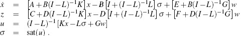
The solution can be obtained when I — ![]() is invertible, which is a necessary condition for well-posedness of the feedback system (3.1). For more information on well-posedness, see Section 3.4.2. The solution is used to write the system (3.1) as
is invertible, which is a necessary condition for well-posedness of the feedback system (3.1). For more information on well-posedness, see Section 3.4.2. The solution is used to write the system (3.1) as

where
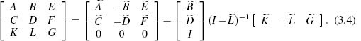
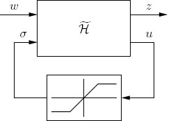
Figure 3.1 A closed-loop system involving a saturation nonlinearity.

Figure 3.2 A closed-loop system involving a saturation nonlinearity written in compact form in negative feedback with a deadzone nonlinearity.
3.1.2 Quadratic functions and semidefinite matrices
The tools used here rely on nonnegative quadratic functions for analysis. Such functions will lead to numerical algorithms that involve solving a set of linear matrix inequalities (LMIs) in order to certify internal stability or quantify external performance. Efficient commercial LMI solvers are widely available.
A nonnegative quadratic function is a mapping x ![]() xTPx where P is symmetric, in other words, P is equivalent to its transpose, and xTPx ≥ 0 for all x. In general, a symmetric matrix P that satisfies xTPx ≥ 0 for all x will be called a positive semidefinite matrix, written mathematically as P ≥ 0. If xTPx> 0 for all x ≠ 0, then P will be called a positive definite matrix, written mathematically as P> 0. A symmetric matrix Q is negative semidefinite, written mathematically as Q ≤ 0, if –Q is positive semidefinite. A similar definition applies for a negative definite matrix. All of these terms are reserved for symmetric matrices. The reason for this is that a general square matrix Z can be written as Z = S+N where S is symmetric, and N is anti-symmetric, i.e., N = –NT, and then it follows that xTZx = xTSx. In other words, the anti-symmetric part plays no role in determining the sign of xTZx. The notation P1> P2, respectively P1 ≥ P2, indicates that the matrix P1 – P2 is positive definite, respectively positive semidefinite. Note that if P> 0, then there exists ε> 0 sufficiently small so that P> εI.
xTPx where P is symmetric, in other words, P is equivalent to its transpose, and xTPx ≥ 0 for all x. In general, a symmetric matrix P that satisfies xTPx ≥ 0 for all x will be called a positive semidefinite matrix, written mathematically as P ≥ 0. If xTPx> 0 for all x ≠ 0, then P will be called a positive definite matrix, written mathematically as P> 0. A symmetric matrix Q is negative semidefinite, written mathematically as Q ≤ 0, if –Q is positive semidefinite. A similar definition applies for a negative definite matrix. All of these terms are reserved for symmetric matrices. The reason for this is that a general square matrix Z can be written as Z = S+N where S is symmetric, and N is anti-symmetric, i.e., N = –NT, and then it follows that xTZx = xTSx. In other words, the anti-symmetric part plays no role in determining the sign of xTZx. The notation P1> P2, respectively P1 ≥ P2, indicates that the matrix P1 – P2 is positive definite, respectively positive semidefinite. Note that if P> 0, then there exists ε> 0 sufficiently small so that P> εI.
3.2 UNCONSTRAINED FEEDBACK SYSTEMS
To set the stage for results regarding the system (3.3), consider using quadratic functions to analyze unconstrained feedback systems, where the saturation nonlinearity in (3.3) is replaced by the identity function, in other words, q ≡ 0, so that the system (3.3) becomes
3.2.1 Internal stability
When checking internal stability, w is set to zero, z plays no role, and (3.5) becomes simply ![]() = Ax. To certify exponential stability for the origin of this system, one method that generalizes to feedback loops with input saturation involves finding a nonnegative quadratic function that strictly decreases along solutions, except at the origin. Quadratic functions are convenient because they lead to stability tests that involve only linear algebra.
= Ax. To certify exponential stability for the origin of this system, one method that generalizes to feedback loops with input saturation involves finding a nonnegative quadratic function that strictly decreases along solutions, except at the origin. Quadratic functions are convenient because they lead to stability tests that involve only linear algebra.
To determine whether a function is decreasing along solutions, it is enough to check whether, when evaluated along solutions, the function's time derivative is negative. For a continuously differentiable function, the time derivative can be obtained by computing the directional derivative of the function in the direction Ax and then evaluating this function along the solution. This corresponds to the mathematical equation
where V represents the function, ![]() represents its time derivative along solutions at time t, ∇V(x) is the gradient of the function, and (∇V(x), Ax) is the directional derivative of the function in the direction Ax. For a quadratic function V(x) = xTPx, where P is a symmetric matrix, the classic chain rule gives that this directional derivative equals
represents its time derivative along solutions at time t, ∇V(x) is the gradient of the function, and (∇V(x), Ax) is the directional derivative of the function in the direction Ax. For a quadratic function V(x) = xTPx, where P is a symmetric matrix, the classic chain rule gives that this directional derivative equals
xT (PA + ATP)x.
Thus, in order for the time derivative to be negative along solutions, except at the origin, it should be the case that the directional derivative satisfies
xT(ATP + PA)x < 0 ∀x ≠ 0,
in other words, ATP + PA < 0. In summary, to certify internal stability for the system (3.5) with a given matrix A, one looks for a symmetric matrix P satisfying
P ≥ 0
This is a particular example of a set of LMIs, which will be discussed in more detail in Section 3.3 Software for checking the feasibility of LMIs is widely available It turns out that the LMIs in (3.6) are feasible if and only if the system (3.5) is internally stable
Now the external disturbance w is no longer constrained to be zero. Thus, the relevant equation is (3.5). The goal is to determine the L2 gain from disturbance w to the performance output variable z and simultaneously establish internal stability. It is possible to give an arbitrarily tight upper bound on this gain by again exploiting nonnegative quadratic functions. However, the quadratic function will not always be decreasing along solutions. Instead, an upper bound on the time derivative will be integrated to derive a relationship between the energy in the disturbance w and the energy in the performance output variable z. Again, the directional derivative of the function xTPx in the direction Ax + Ew generates the time derivative of the function along solutions. This time the directional derivative is given by
xT(ATP+PA)x+2xTPEw.
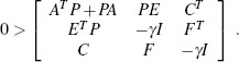
In order to guarantee an L2 gain less than a number γ > 0 and to establish internal stability at the same time, it is sufficient to have
Using the definition of z in (3.5), this condition is the same as having, for all (x, w) ≠ 0,
In other words, the large matrix in the middle of this expression is negative definite. In summary, to certify internal stability and L2 external stability with gain less than γ > 0 for the system (3.5) with a given set of matrices (A, B, E, F), it suffices to find a symmetric matrix P satisfying

This is another set of LMIs, the feasibility of which can be tested with standard commercial software. Moreover, such software can be used to approximate the smallest possible number γ that makes the LMIs feasible. The feasibility of the LMIs in (3.8) is also necessary for the L2 gain to be less than y with internal stability.
3.3 LINEAR MATRIX INEQUALITIES
As the preceding sections show, the analysis of dynamical systems benefits greatly from the availability of software to solve LMIs. The sections that follow show that LMIs also arise when using quadratic functions to analyze feedback loops with saturation. LMIs also appear in most of the anti-windup synthesis algorithms given in this book. The goal of this section is to provide some familiarity with LMIs and to highlight some aspects to be aware of when using LMI solvers.
Linear matrix inequalities are generalizations of linear scalar inequalities. A simple example of a linear scalar inequality is
where a and q are known parameters and z is a free variable. In contrast to the linear scalar equality 2za + q = 0, which either admits no solution (if a = 0 and q ≠ 0), an infinite number of solutions (if a = 0 and q ≠ 0), or one solution (if a ≠ 0), the linear scalar inequality (3.9) either admits no solutions (if a = 0 and q ≥ 0) or admits a convex set of solutions given by ![]() In the former case the inequality is said to be infeasible. In the latter case it is said to be feasible.
In the former case the inequality is said to be infeasible. In the latter case it is said to be feasible.
Linear matrix inequalities generalize linear scalar inequalities by allowing the free variables to be matrices, allowing the expressions in which the free variables appear to be symmetric matrices, and generalizing negativity or positivity conditions to negative or positive definite matrix conditions.
Replacing the quantities in (3.9) with their matrix counterparts and insisting that the resulting matrix be symmetric gives the linear matrix inequality
In this LMI, A and Q are known matrices and Q is symmetric. The matrix Z comprises m times n free variables where m denotes the number of columns of Z and n denotes the number of rows of Z. Characterizing the solution set of (3.10) is not as easy as before, because the solution space will be delimited by several hyperplanes that depend on the entries of the matrices A and Q. However, one important property of this solution set is that it is convex. In particular, if the matrices {Z1,…, Zk} all satisfy the LMI (3.10) then for any set of numbers {λ1,…,λk}, where each of these numbers is between zero and one, inclusive, and the sum of the numbers is one, the matrix
also satisfies the LMI (3.10). The convexity property arises from the fact that (3.10) is linear in the free variable Z.
Now consider the case where Q is taken to be zero and the free variable Z is required to be symmetric and positive semidefinite. The variable Z will be replaced by the variable P for this case. With the free variable being symmetric, the parameter A is now required to be a square matrix. Now, recall that the matrix condition ATP + PA < 0 is equivalent to the existence of ε> 0 such that ATP + PA + εI ≤ 0. Therefore, an extra free variable e can be introduced to write the overall conditions as the single LMI
The implicit constraint that P is symmetric reduces the number of free variables in the matrix P to the quantity n(n + 1)/2, where n is the size of the square matrix P. The feasibility of the LMI (3.11) is equivalent to the simultaneous feasibility of the two LMIs
which match the LMIs (3.6) that appeared in the analysis of internal stability for linear systems. It is worth noting that most LMI solvers have difficulty with inequalities that are not strict. This is because sometimes, in this case, the feasibility is not robust to small changes in the parameters of the LMI. For example, with the choice
the LMIs P > 0 and 0 ≥ ATP + PA are feasible (note that the strictly inequality and the nonstrict inequality have been exchanged relative to (3.12) as can be seen by taking P = I. However, the LMIs are not feasible if one adds to A the matrix εl for any ε > 0. On the other hand, strict LMIs, if feasible, are always robustly feasible. Fortunately, the feasibility of the LMIs (3.12) is equivalent to the feasibility of the LMIs
This can be verified by letting ![]() denote a feasible solution to (3.12) and observing that
denote a feasible solution to (3.12) and observing that ![]() + εl must be a feasible solution to (3.13) for ε > 0 sufficiently small. From the discussion in Section 3.2.1, it follows that the LMIs (3.13) are feasible if and only if the system
+ εl must be a feasible solution to (3.13) for ε > 0 sufficiently small. From the discussion in Section 3.2.1, it follows that the LMIs (3.13) are feasible if and only if the system ![]() = Ax is internally stable.
= Ax is internally stable.
Next consider the matrix conditions that appeared in Section 3.2.2, the feasibility of which was equivalent to having L2 external stability with gain less than γ> 0 and internal stability for (3.5). Using the same idea as above to pass to a strict inequality for the matrix P, the feasibility of the matrix conditions in (3.8) is equivalent to the feasibility of the matrix conditions

The matrices (A,E, C,F) are parameters that define the problem. If the value y is specified, then the feasibility of the resulting LMIs in terms of the free variable P can be checked with an LMI solver. If the interest is in finding values for y 0 to make the matrix conditions feasible, then y can be taken to be a free variable. However, the matrix conditions do not constitute LMIs because of the nonlinear dependence on the free parameter y through the factor 1/y that appears. Fortunately, there is a way to convert the matrix conditions above into LMIs in the free variables y and P using the following fact:
(Schur complements) Let Q and R be symmetric matrices and let S have the same number of rows as Q and the same number of columns as R. Then the matrix condition
is equivalent to the matrix conditions
This fact can be applied to the matrix conditions (3.14) to obtain the matrix conditions

which are LMIs in the free variables P and γ. If the system ![]() = Ax is internally stable, then these LMIs will be feasible. This follows from the fact that there will exist P > 0 satisfying ATP + PA < 0, which is the matrix that appears in the upper left-hand corner of the large matrix in (3.15), and a consequence of Finsler's lemma, which is the following:
= Ax is internally stable, then these LMIs will be feasible. This follows from the fact that there will exist P > 0 satisfying ATP + PA < 0, which is the matrix that appears in the upper left-hand corner of the large matrix in (3.15), and a consequence of Finsler's lemma, which is the following:
(Finsler's lemma) Let Q be symmetric and let H have the same number of columns as Q. If ζTQζ < 0 for all ζ ≠ 0 satisfying Hζ = 0, then, for all γ> 0 sufficiently large, Q — γHTH < 0.
If one applies this fact with the matrix

and

one sees that the LMIs in (3.15) will be feasible for an appropriate P matrix and large enough γ > 0.
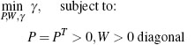
To determine a tight upper bound on the L2 gain, one is interested in making γ as small as possible. The task of minimizing γ subject to satisfying the LMIs (3.15) is an example of an LMl eigenvalue problem and can be written as:
 (3.16b)
Since large block matrices that appear in LMIs must always be symmetric, the entries below the diagonal must be equal to the transposes of the entries above the diagonal. For this reason, such matrices can be replaced with the “*” symbol without any loss of information. For example, (3.16) can be written as
 (3.17b)
with no loss of information.
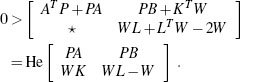
An alternative notation that may simplify (3.16) relies on the use of the function “He” which, given any square matrix X, is defined as HeX := X + XT, so that (3.16) can be written as

The LMI feasibility and eigenvalue problems can be solved efficiently using modern numerical software packages. As an example, the code needed in MAT-LAB's LMI control toolbox to implement the search for the optimal solution to (3.16) or, equivalently, of (3.17) and (3.18), is given next.
Example 3.3.1 Implementing LMIs using MATLAB's LMI control toolbox requires first defining the LMI constraints structure and then running the solver on those constraints. The LMI constraints are specified by a start line (setlmis ([]);) and an end line (mylmisys-getlmis;) which also gives a name to the LMI constraints. Then the LMI constraints consist of a first block where the LMI variables are listed and of a second block where the LMI constraints are described in terms of those variables. The following code gives a rough idea of how this should be implemented. Comments within the code provide indications of where the different blocks are located. For more details, the reader should refer to MATLAB's LMI control toolbox user's guide.


![]()
Example 3.3.2 The MATLAB code illustrated in the previous example is quite streamlined and using the LMI control toolbox in such a direct way can many times become quite complicated in terms of actual MATLAB code. An alternative to this is to indirectly specify the LMI constraints and use the LMI control toolbox solver by way of the YALMIP (=Yet Another LMI Parser) front-end. The advantages of using YALMIP mainly reside in the increased simplicity of the code (thereby significantly reducing the probability of typos) and in the code portability to alternative solvers to the classic LMI control toolbox (SeDuMi is a much used alternative). The same calculation reported in the previous example is computed using the YALMIP front-end in the following code:

Example 3.3.3 CVX is another useful program for solving structured convex optimization problems, including LMIs. The previous calculations in CVX are as follows:
![]()


There are a few points to make about the variability in solutions to LMI eigenvalue problems returned by using different commercial solvers. First, notice that the LMI eigenvalue problem in (3.17) involves an optimization over an open set of matrices. So, technically, it is not possible to achieve the minimum. It would be more appropriate to say that the optimization problem is looking for the infimum. Indeed, if a minimum γ* existed and satisfied the LMIs, then it would also be the case that γ — ε satisfied the LMIs for ε > 0 sufficiently small, contradicting the fact that γ* is a minimum. A consequence of this fact is that, since it is not possible to reach an infimum, each solver will need to make its own decision about the path to take toward the infimum and at what point to stop. Different paths to the infimum and different stopping conditions will cause different solvers to return different solutions. Second, unless the optimization is strictly convex, the solution to the optimization problem may be nonunique. This fact may also contribute to variability in the solutions returned by different solvers. In each of these cases, the different minima returned should be quite close to one another, whereas the matrices returned that satisfy the LMIs may be quite different. In anti-windup synthesis, these differences may lead to different anti-windup compensator matrices. Therefore, when trying to reproduce the results in the later examples, one may find that the compensators determined with a particular software package are very different from the ones found in the book. Nevertheless, the responses induced by the compensators should be very similar to the ones reported herein. In particular, the performance metric for which the compensator was designed should be very nearly the same.
Before moving on to the analysis of constrained feedback systems, one additional matrix manipulation, which will be used to analyze systems with saturation, will be introduced. It is closely related to Finsler's lemma.
(S-procedure) Let Mo and M1 be symmetric matrices and suppose there exists ζ* such that ζ*M1ζ*> 0. Then the following statements are equivalent:
i. There exists τ> 0 such that M0 — τM1> 0.
ii. ZTM0Z> 0 for all Z = 0 such that ZTM1 Z > 0.
The implication from (i) to (ii) is simple to see, and does not require the existence of ζ* such that ζ*M1 ζ*> 0. The opposite implication is nontrivial.
3.4 CONSTRAINED FEEDBACK SYSTEMS: GLOBAL ANALYSIS
3.4.1 Sector characterizations of nonlinearities
In order to arrive at LMIs when checking the internal stability and L2 external stability for feedback loops with saturations or deadzones, one typically inscribes the saturation or deadzone into a conic region and applies the S-procedure. To understand the idea behind inscribing a nonlinearity into a conic region, consider a scalar saturation function. Figure 3.3 contains, on the left, the block diagram of the saturation function and, on the right, the graph of the saturation function. The figure emphasizes that the graph of the saturation function is contained in a conic sector delimited by the line passing through the origin with slope zero and the line passing through the origin with slope one. The deadzone nonlinearity, as shown in Figure 3.4, is also contained in this sector. In fact, the sector contains any scalar nonlinearity with the property that its output y always has the same sign as its input u and y has a magnitude that is never bigger than that of u. This condition can be expressed mathematically using the quadratic inequality y(u — y)> 0, which, when focusing on the deadzone nonlinearity where y = q, becomes
q(u — q) ≥ 0.
This condition says that qu ≥ q2, which captures the sign and magnitude information described above.

Figure 3.3 The scalar saturation function and its sector properties.
For a decentralized nonlinearity where each component of the nonlinearity is inscribed in the sector described above, the quadratic condition holds, where qi are the components of the output vector y, ui are the components of the input vector u, and wi are arbitrary positive weightings. This can also be written as

Figure 3.4 The scalar deadzone function and its sector properties.
where W is a diagonal matrix consisting of the values wi.
A sector characterization of nonlinearities introduces some conservativeness since the analysis using sectors will apply to any nonlinearity inscribed in the sector. The payoff in using sector characterizations is that the mathematical description, in terms of quadratic inequalities, is compatible with the analysis of feedback systems using quadratic functions. Indeed, the S-procedure described earlier permits combining the quadratic inequality describing the sector with the quadratic inequalities involved in the directional derivative to arrive at LMIs for the analysis of feedback loops with sector nonlinearities. This will be done subsequently.
3.4.2 Guaranteeing well-posedness
Before analyzing the feedback loop given by (3.3), shown in Figure 3.2, it must be established that the feedback loop is well-posed. In particular, it should be verified that the equation
u — L(u − sat(u)) = v
admits a solution u for each v and that the solution u(v) is a sufficiently regular function of v. When sat (u) is decentralized, the equation admits a solution that is a Lipschitz function of v when each of the matrices
is invertible. It turns out that each of these matrices is invertible when there exists a diagonal, positive definite matrix W such that
LTW + WL — 2W < 0. (3.20)
This LMI in W will appear naturally in the analysis LMIs in the following sections. The LMI can be strengthened by replacing the “2” with a smaller positive number in order to guarantee that the feedback loop is not too close to being ill-posed. In particular, in many of the algorithms proposed later in this book, the following LMI will be employed:
LTW + WL — 2(1 — v)W < 0, (3.21)
or equivalent versions of it. This LMI is referred to as a strong well-posedness constraint and enforces a bound on the speed of variation of the closed-loop state (by bounding the Lipschitz constant of the right-hand side of the dynamic equation).
3.4.3 Internal stability
To analyze internal stability for (3.3), set w = 0 and consider the resulting system, which is given by

Again, a nonnegative quadratic function V(x) = xTPx will be used. Like in the case of linear systems, it is desirable for the time derivative of V(x(t)) to be negative except at the origin. The time derivative is obtained from the directional derivative of V(x) in the direction Ax + Bq, which is given by
(∇V(x), Ax + Bq) = xT (ATP + PA)x+2xTPBq.(3.23)
Since q is the output of the deadzone nonlinearity, it follows from the discussion in Section 3.4.1 that the property
qTW(u — q) ≥ 0
holds for any diagonal positive semidefinite matrix W. Then, using the definition of u in (3.22), the requirement on the time derivative translates to the condition
In order to guarantee this implication, it is enough to check that
This is the easy implication of the S-procedure, where the T has been absorbed into the free variable W. In fact, the S-procedure can be used to understand that there is no loss of generality in replacing (3.24) by (3.25). The condition (3.25) can be written equivalently as

In other words,
This condition is an LMI in the free variables P, which should be positive semidef-inite, and W, which should be diagonal and positive definite. The matrices (A, B, K, L) are parameters that define the system (3.22). Notice that, because of the lower right-hand entry in the matrix, the LMI condition for well-posedness given in Section 3.4.2 is automatically guaranteed when (3.27) is satisfied. In addition, because of the upper left-hand entry in the matrix, the matrix A must be such that the linear system ![]() = Ax is internally stable. Finally, note that the LMI condition is not necessary for internal stability. For example, consider the system
= Ax is internally stable. Finally, note that the LMI condition is not necessary for internal stability. For example, consider the system

The LMI for internal stability becomes
or, equivalently,
In order for this matrix to be positive definite, the determinant of the matrix, given by 4pw − (p + w)2, must be positive. However, 4pw − (p + w)2= − (p − w)2 which is never positive. Therefore, the internal stability LMI is not feasible. Nevertheless, the system is internally stable since the system is equivalent to the system
for which the quadratic function V(x) = x2 decreases along solutions but not at a quadratic rate.
In general, the LMI for internal stability for the system (3.3) will not be feasible if the linear system ![]() = [A + B(I — L)-1K]x is not internally stable. This is the system that results from (3.3) by setting w = 0 and sat(u) ≡ 0. To put it another way, when the system (3.3) is expressed as a feedback interconnection of a linear system with a saturation nonlinearity rather than a deadzone, the resulting system is
= [A + B(I — L)-1K]x is not internally stable. This is the system that results from (3.3) by setting w = 0 and sat(u) ≡ 0. To put it another way, when the system (3.3) is expressed as a feedback interconnection of a linear system with a saturation nonlinearity rather than a deadzone, the resulting system is
Then, for the LMI-based internal stability test in (3.27) to be feasible, it is necessary that (3.32) with σ = 0 and w = 0 be internally stable.
3.4.4 External stability
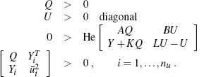
Now consider establishing L2 external stability for the system (3.3). Again relying on a nonnegative quadratic function, and combining the ideas in Sections 3.2.2 and 3.4.3, it is sufficient to have that
qTW(Gw + Kx + Lq - q) ≥ 0, (x, q, w) ≠ 0
Then, using the definition of z, and applying the S-procedure and Schur complements, produces the condition
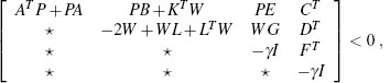
which is an LMI in the unknowns P = PT> 0, W> 0 diagonal and γ> 0. The four blocks in the upper left corner correspond to the LMI for internal stability given in (3.27). It follows that if the system (3.3) is internally stable, then the LMI (3.34) is feasible using the solutions P and W from the internal stability LMI and then picking γ> 0 sufficiently large. Of course, the goal is to see how small 7 can be chosen. This objective corresponds to solving the eigenvalue problem
 (3.35b)
Since a necessary condition for global internal and external stability for the system (3.3) is that the matrix A + B(I - L)-lK be exponentially stable, there will be many situations where the LMIs given in this section will not be feasible. For this reason, it is helpful to have a generalization of these results for the case where only regional internal and external stability can be established. This is the topic of the next section.
3.5 CONSTRAINED FEEDBACK SYSTEMS: REGIONAL ANALYSIS
3.5.1 Regional sectors
To produce LMI results that are helpful for a regional analysis of systems with saturation, it is necessary to come up with a tighter sector characterization of the saturation nonlinearity while still using quadratic inequalities. This appears to be impossible to do globally. However, for analysis over a bounded region, there is a way to make progress. For the scalar saturation function, one fruitful idea is to take H to be an arbitrary row vector and note that the quadratic inequality
will hold for any input-output pairs u and σ generated by the saturation nonlinearity. This can be verified by checking two cases:
1. If σ := sat(u) = u, then σ = u, and so the quadratic form on the left-hand side is zero.
2. If sat(u) ≠ u, then the sign of (u - σ) is equal to the sign of u and also the sign of σ + Hx is equal to the sign of u so that the product is not negative. The condition sat(Hx) = Hx is used in this step.
The corresponding condition for the deadzone nonlinearity having input u and output q can be derived from (3.36) by using the definition q := dz(u) = u–sat(u) = u – σ. The resulting quadratic condition is
The decentralized vector version of this inequality is
where H is now a matrix of appropriate dimensions and W is a diagonal, positive definite matrix. In order to have sat(Hx) = Hx for all possible values of x, it must be the case that H = 0. In this case, the sector condition in (3.38) reduces to the global sector condition used previously.
3.5.2 Internal stability
In this section, the sector characterization of the previous section is exploited. The saturation nonlinearity is taken to be decentralized, the saturation limits are taken to be symmetric, and the ith function is limited in range to ±![]() i. In order to guarantee the condition sat(Hx(t)) = Hx(t) for solutions to be considered, which is needed to exploit the sector condition of the previous section, the condition
i. In order to guarantee the condition sat(Hx(t)) = Hx(t) for solutions to be considered, which is needed to exploit the sector condition of the previous section, the condition
is imposed, where Hi denotes the ith row of H. Using Schur complements, the condition (3.39) can be written as the matrix condition
According to (3.39), xTPx ≤ 1 implies sat(Hx) = Hx. So, the analysis of internal stability can now proceed like before but restricting attention to values of x for which xTPx ≤ 1 and using the sector condition from the previous section. Indeed, if in the set ε(P) := {x: xTPx ≤ 1} the quadratic function xTPx is decreasing along solutions, then the set ε will be forward invariant and convergence to the origin will ensue.
Picking up the analysis from Section 3.4.3 immediately after the description of the directional derivative of the quadratic function xTPx in the direction Ax + Bq in equation (3.23), the condition (3.24) is now replaced by the condition
In order to guarantee this implication, it is enough to check that, for all (x, q) ≠ 0,
The condition (3.42) can be written equivalently as
In other words,
The matrix conditions that can then be used to establish internal stability over the region ε (P) are given by (3.40) and (3.44) together with P> 0, W> 0 and the condition that W is diagonal. These conditions are not linear in the free variables P, W, and H. In particular, notice the term HTW that appears in the upper right-hand corner of the matrix in (3.44). Nevertheless, there is a nonlinear transformation of the free variables that results in an LMI condition. The transformation exploits the fact that the condition S < 0 is equivalent to the condition RTSR < 0 for any invertible matrix R. Make the definitions Q := P-1, U := W-1, and Y := HQ. These definitions make sense since W and P must be positive definite. Moreover, P, W, and H can be recovered from Q, U, and Y. Now observe that
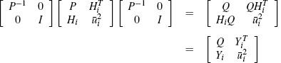
and

Thus, internal stability over the region ε(Q-1feasible in the free parameters Q, U, and Y:
Moreover, it is possible to use these LMIs as constraints for optimizing the set ε(Q-1) in some way. In the next section, LMIs will be given for establishing internal stability and minimizing the L2 external gain over a region. Numerical examples will be given there.
3.5.3 External stability
Consider establishing L2 external stability for the system (3.3) over a region. The initial condition will be taken to be zero and the size of the solution x(t) will be limited by limiting the energy in the disturbance input w. In particular, if it is true that
whenever x(t)TPx(t) ≤ s2, and if ||w||2 ≤ s, then it follows by integrating this inequality that
Thus, changing the bound in (3.39) to
will guarantee that sat (Hx(t)) = Hx(t) for all disturbances w with ||w||2 ≤ s. The condition (3.50) corresponds to the matrix condition
The appropriate condition on the derivative of the function x Px is guaranteed by the fact that condition
implie
which generalizes the inequalities (3.7) and (3.33) addressing the same problem, respectively for the case without saturation and for the case with a global sector bound on the saturation. As compared to (3.7) and (3.33), the right-hand side of the inequality above is divided by γ. This is a key fact which allows writing inequality (3.49) independently of Y and therefore to derive the LMIs (3.54) below for the regional L2 gain computation.
Using the definition of z, and applying the S-procedure and Schur complements, produces the matrix conditions

The four blocks in the upper left corner correspond to the LMI for internal stability given in (3.44). As before, the matrix conditions (3.51) and (3.53) are not linear in
the free variables P, W, and H. Again, notice the HTW term that appears but that the matrix conditions can be reformulated as LMIs through a nonlinear transformation on the free variables. Using the same transformation as in the case for internal stability, the following LMIs are obtained in the free variables Q, U, and Y:
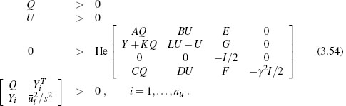
The minimum γ2> 0 for which the LMIs are feasible is a nondecreasing function of s. An upper bound on the nonlinear gain from ||w||2 to ||z||2 can be established by solving the LMI eigenvalue problem of minimizing γ2 subject to the LMIs (3.54) for a wide range of values for s and plotting γ as a function of s. This procedure generates the function ![]() mentioned in Section 2.4.4. The function rdescribed in Section 2.4.4 is given by s
mentioned in Section 2.4.4. The function rdescribed in Section 2.4.4 is given by s![]() (s).
(s).
3.6 ANALYSIS EXAMPLES
In this section, a few examples of nonlinear gain computation are provided to illustrate the use of the LMIs (3.54). The second example is taken from subsequent chapters, where anti-windup problems are solved.
Example 3.6.1 Consider a one-dimensional plant stabilized by negative feedback through a unit saturation and subject to a scalar disturbance w. The closed-loop dynamic equation is given by
![]() p = axp + sat(u) + w
p = axp + sat(u) + w
u = −(a + 10)xp,
which can be written in terms of the deadzone function as
q = dz((a + 10)xp).
System (3.55) will be analyzed in three main cases:
1. a = 1, which resembles an exponentially unstable plant stabilized through a saturated loop; this case has been considered on page 28 when discussing regional external stability;
2. a = 0, which represents an integrator, namely a marginally stable plant stabilized through a saturated loop; this case has been considered on page 30 when characterizing unrecoverable responses;
3. a = -1, which represents an exponentially stable plant whose speed of convergence is increased through a saturated loop; this case has been considered on page 62 when illustrating LMI-based internal stability tests.
The three cases listed above have been used to generate, respectively, the nonlinear gains in Figures 2.17, 2.18, and 2.20 on page 45 when first introducing nonlinear performance measures.
When adopting the representation (3.3), system (3.55) is described by the following selection, with z = xp:


Figure 3.5 Nonlinear L2 gains for the three cases considered in Example 3.6.1.
The matrices (3.56) can be used in the LMI conditions (3.54) for different values of s, to compute the nonlinear gains for the three cases under consideration. The resulting curves are shown in Figure 3.5, where it is possible to appreciate the three different behaviors noted in Section 2.4.4 on page 44 and characterizing exponentially unstable plants, nonexponentially unstable plants with poles on the imaginary axis, and exponentially stable plants. ![]()
Example 3.6.2(SISO academic example no. 2) This example will receive attention in the following chapter. Different solutions to the corresponding windup problem are given in later chapters. Here, the nonlinear gains characterizing the different solutions will be computed by employing the LMI conditions (3.54).
The nonlinear L2 gains corresponding to the following closed loops are comparatively shown in Figure 3.6:
1. Saturated closed loop without anti-windup compensation. Based on the problem data given in Example 4.3.4 on page 89, the closed loop corresponds to:

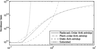
Figure 3.6 Nonlinear L2 gains for Example 3.6.2.
and the resulting nonlinear gain is represented by the dotted curve in Figure 3.6.
2. Closed loop with static regional anti-windup compensation. Based on the problem solution given in Example 4.4.2 on page 104, the closed loop corresponds to:

and the resulting nonlinear gain is represented by the dashed curve in Figure 3.6.
3. Closed loop with full-order dynamic global anti-windup compensation. Based on the problem solution given in Example 5.4.3 on page 119, the closed loop corresponds to:

and the resulting nonlinear gain is represented by the dashed-dotted curve in Figure 3.6.
4. Closed loop with reduced-order dynamic global anti-windup compensation. Based on the problem solution given in Example 5.4.5 on page 128, the closed loop corresponds to:

and the resulting nonlinear gain is represented by the solid curve in Figure 3.6.
![]()
3.7 REGIONAL SYNTHESIS FOR EXTERNAL STABILITY
This section addresses synthesis in feedback loops with saturation based on the LMIs that were derived earlier in this chapter. Only the case of regional L2 external stability is described. The purpose of this section is to give an indication of the types of calculations that arise in the synthesis of anti-windup algorithms.
3.7.1 LMI formulations of anti-windup synthesis
In typical anti-windup synthesis, the designer can inject the deadzone nonlinearity, driven by the control input, at various places in the feedback loop and can also inject the state of a filter driven by the deadzone nonlinearity. Letting x denote the composite state of the plant having np components, unconstrained controller having nc components, and anti-windup filter having naw components, the synthesis problem can be written as

where the design parameters are K1, K2, Φ1 and Φ2. All of the other matrices are fixed by the problem description, coming either from the plant model or the model of the unconstrained controller and are overlined for notational convenience. Typically, ![]() 1x represents the states of the anti-windup augmentation filter. The design parameters K1 and K2 determine how those states are used to determine the characteristics of the filter and the injected terms in the controller. When using static anti-windup augmentation, which corresponds to the case where there are no states in the anti-windup augmentation filter, the matrices K1 and K2 are set to zero. The design parameters Φ1 and Φ2 determine how the deadzone nonlinearity is injected into the state equations and controller. The matrix
1x represents the states of the anti-windup augmentation filter. The design parameters K1 and K2 determine how those states are used to determine the characteristics of the filter and the injected terms in the controller. When using static anti-windup augmentation, which corresponds to the case where there are no states in the anti-windup augmentation filter, the matrices K1 and K2 are set to zero. The design parameters Φ1 and Φ2 determine how the deadzone nonlinearity is injected into the state equations and controller. The matrix ![]() 1 limits where the states of the anti-windup filter and the deadzone nonlinearity can be injected into the dynamical equations.
1 limits where the states of the anti-windup filter and the deadzone nonlinearity can be injected into the dynamical equations.
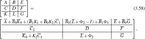
the system (3.57) agrees with the system (3.3) and the corresponding regional performance analysis LMI from Section 3.5.3 is

Since some of the components of A, B, K, and L are free for design, these matrices are replaced in (3.59) by their definitions from (3.58). The additional definitions
give relationships between Φi and Θi for i ∈ {1,2} that are invertible because U is positive definite by assumption. Using these definitions, the matrix conditions (3.59) become

In the case of static anti-windup augmentation, where K1 = 0 and K2 = 0, the conditions (3.61) constitute LMIs in the free variables U, Q, ![]() 1,
1, ![]() 2, and γ. Note that in (3.6) all the ixed parameters are overlined and all the free variables are not.
2, and γ. Note that in (3.6) all the ixed parameters are overlined and all the free variables are not.
For some problems related to anti-windup synthesis, ![]() is invertible and then, with the definitions
is invertible and then, with the definitions
which give an invertible relationship between Ki and Xi, i ∈ {1,2}, the conditions (3.61) constitute LMIs in the free variables U, Q, ![]() 1,
1, ![]() 2, X1, X2, and γ.
2, X1, X2, and γ.
In the more typical situation where C1 is not invertible, a different approach can be taken to eliminate the nonlinear terms that involve products of Q and Ki, i G {1,2}, at least when the size of the anti-windup augmentation filter has the same number of states as the plant model. In this situation, define
and construct matrices Ψ, H, and G such that the conditions (3.61) become
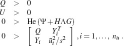
According to the “elimination lemma” from linear algebra, there exists a value Λsatisfying 0> He (Ψ + HΛG) if and only if
where WH and WG are any full-rank matrices satisfying ![]()
Then, exploiting the special structure of anti-windup problems, the matrices Q and Y can be partitioned as

where R11 is an np×np matrix, R22 is an nc ×nc matrix, and M is an naw ×naw matrix, and it can be verified that ![]() < 0 is an LMI in R11 and Z, while
< 0 is an LMI in R11 and Z, while ![]() < 0 is an LMI in S. Then, as long as R11 and S satisfy the condition R11−S11> 0, which is another LMI in R11 and S, it is always possible to pick R12, R22, N, and M so that PQ = I. Finally, as long as
< 0 is an LMI in S. Then, as long as R11 and S satisfy the condition R11−S11> 0, which is another LMI in R11 and S, it is always possible to pick R12, R22, N, and M so that PQ = I. Finally, as long as
which is yet another LMI in R11 and Z, it is always possible to pick Yb and Yc so that
Finally, with Y and Q generated, it is possible to find Λ and U such that 0> He (Ψ + HΛG).
3.7.2 Restricting the size of matrices
It is sometimes convenient to restrict the size of the matrices determined by the LMI solver when seeking for optimal solutions minimizing the gain γ2 in (3.61). Indeed, it may sometimes happen that minimizing the gain leads the LMI solver in a direction where certain parameters become extremely large providing very little performance increase. To avoid this undesirable behavior, it is often convenient to restrict the size of the free variables in (3.61) by incorporating extra constraints in the LMI optimization.
Given any free matrix variable M, one way to restrict its entries is to impose a bound k on its maximum singular value, namely, impose
MTM < k2I.
This can be done by dividing the equation above by k and applying a Schur complement to ![]() which gives:
which gives:
This type of solution can be used, for example, to restrict the size of the anti-windup matrices K1, K2, Ψ1 and Ψ2 in (3.61). In particular, this is achieved by imposing
where Λ is defined in equation (3.63). Then, since by (3.60)
the anti-windup parameters will satisfy![]() denotes the maximum singular value of its argument.
denotes the maximum singular value of its argument.
Notice that imposing the extra constraints (3.66) reduces the feasibility set of the synthesis LMIs and conservatively enforces the bound on the anti-windup matrices (because it also restricts the set of allowable free variables U). However, it works well in many practical cases, as illustrated in some of the examples discussed in the following chapters.
3.8 NOTES AND REFERENCES
LMIs have played a foundational role in analysis and control of dynamical systems for several decades. A comprehensive book on this topic is the classic [G17], where an extensive list of references can be found. That book also contains the facts quoted herein concerning Schur complements, the Finsler lemma, the S-procedure, and the elimination lemma. The analysis of Section 3.4 corresponds to the MIMO version of the classical circle criterion in state-space form. The regional analysis of Section 3.5 is primarily due to the generalized sector condition introduced in [SAT11] and [MI27].
The global and regional analysis discussed in Sections 3.4 and 3.5 corresponds to the quadratic results of [SAT15], where nonquadratic stability and L2 performance estimates are also given. The synthesis method of Section 3.7 corresponds to the regional techniques of [MI33] for the most general case, but previous papers followed that approach for anti-windup synthesis: the static global design of [MI11], the dynamic global design of [MI18, MI26] and its external extension in [MI22], the discrete-time results of [MI24] and [MI30]. The elimination lemma used in Section 3.7 can be found in [G17]. It was first used as shown here in the context of LMI-based H∞ controller synthesis. The corresponding techniques appeared simultaneously and independently in [G5] and [G6] (see also [G8] for an explicit solution to the second design step when applying the elimination lemma).
Well-posedness for feedback loops involving saturation nonlinearities has been first addressed in [MR15], where results from [G18] were used to establish sufficient conditions for well-posedness. Similar tools were also used in [MI18], where the well-posedness of the earlier schemes of [MI11] was also proved. The strong well-posedness constraint discussed in Section 3.4.2 arises from the results of [MI20]. More recently, in [SAT15] a further characterization of sufficient only and necessary and sufficient conditions has been given.
Regarding the LMI solvers mentioned in Examples 3.3.1–3.3.3, the LMI control toolbox [G19] of MATLAB can be purchased together with MATLAB. YALMIP [G15] is a modeling language for defining and solving advanced optimization problems. CVX [G1] is a package for specifying and solving convex programs. Both [G15] and CVX [G1] are extensions of MATLAB which can be downloaded from the web for free and easily installed as toolboxes on a MATLAB installation.