
This section deals with how you can reshape data. Sometimes, data is stored in what is known as a stacked format. Here is an example of stacked data using the PlantGrowth dataset:
    In [344]: plantGrowthRawDF=pd.read_csv('./PlantGrowth.csv')
           plantGrowthRawDF
    Out[344]:   observation   weight  group
            0   1      4.17  ctrl
            1   2      5.58  ctrl
            2   3      5.18  ctrl
            ...
            10       1        4.81    trt1
            11       2        4.17    trt1
            12       3        4.41    trt1
           ...
            20       1        6.31    trt2
            21       2        5.12    trt2
            22       3        5.54    trt2
This data consists of results from an experiment that compared the dried weight yields of plants that were obtained under a control (ctrl) and two different treatment conditions (trt1 and trt2). Suppose we wanted to do some analysis on this data by group value. One way to do this would be to use a logical filter on the DataFrame:
    In [346]: plantGrowthRawDF[plantGrowthRawDF['group']=='ctrl']
    Out[346]:   observation   weight  group
            0     1      4.17   ctrl
            1   2      5.58   ctrl
            2   3      5.18   ctrl
            3   4      6.11   ctrl
           ...
This can be tedious, so we would instead like to pivot/unstack this data and display it in a form that is more conducive to analysis. We can do this using the DataFrame.pivot function as follows:
    In [345]: plantGrowthRawDF.pivot(index='observation',columns='group',values='weight')
    Out[345]: weight
              group   ctrl  trt1  trt2
          observation
            1   4.17   4.81   6.31
            2   5.58   4.17   5.12
            3   5.18   4.41   5.54
            4   6.11   3.59   5.50
            5   4.50   5.87   5.37
            6   4.61   3.83   5.29
            7   5.17   6.03   4.92
            8    4.53   4.89   6.15
            9   5.33   4.32   5.80
           10   5.14   4.69   5.26
Here, a DataFrame is created with columns corresponding to the different values of a group, or, in statistical parlance, levels of the factor.
Some more examples of pivoting on salesdata.csv are as follows:
datastr=pd.read_csv('salesdata.csv')
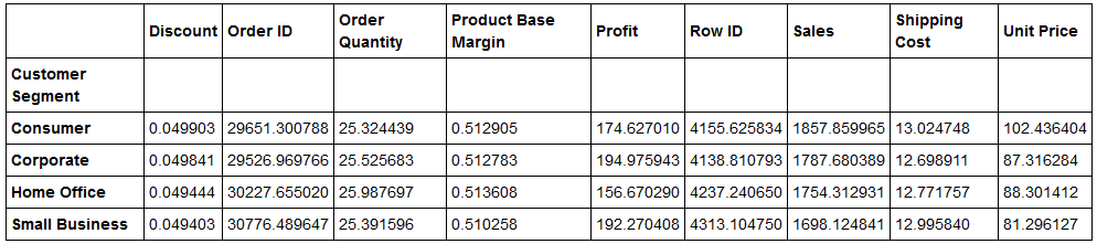
table=pd.pivot_table(datastr,index=['Customer Segment'])# the aggregate values are average by default
The following will be the output. This gives the results for all the columns:
If we specify a columns parameter with a variable name, all the categories in that variable become separate columns:
table2=pd.pivot_table(datastr,values='Sales',index=['Customer Segment'],columns=['Region'])
For example, the output of the preceding code would be as shown following:

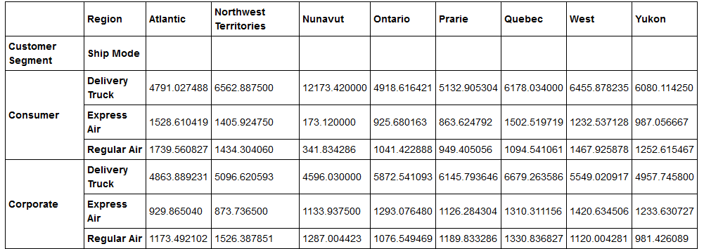
Multi-indexed pivots are also possible, as shown:
table4=pd.pivot_table(datastr,values='Sales',index=['Customer Segment','Ship Mode'],columns=['Region'])
The following will be the output:
A different aggregate function, other than default average, or a custom function can be applied for aggregation as shown in the example following:
table5=pd.pivot_table(datastr,values='Sales',index=['Customer Segment','Ship Mode'],columns=['Region'],aggfunc=sum)
The following will be the output:

Some more important tips and tricks to keep in mind while using pivot_tables are listed following:
- If you expect missing values in your pivot table, then use fill.values=0:
table4=pd.pivot_table(datastr,values='Sales',index=['Customer Segment','Ship Mode'],columns=['Region'],fill_values=0)
- If you want totals at the end, use margins=TRUE:
table4=pd.pivot_table(datastr,values='Sales',index=['Customer Segment','Ship Mode'],columns=['Region'],fill_values=0,margins=TRUE)
- You can pass different aggregate functions to different value columns:
table6=pd.pivot_table(datastr,values=['Sales','Unit Price'],index=['Customer Segment','Ship Mode'],columns=['Region'],aggfunc={"Sales":sum,"Unit Price":len})